The Artificial Mind’s Eye

Abstract

We introduce a novel artificial neural network architecture that integrates robustness to adversarial input in the network structure. The main idea of our approach is to force the network to make predictions on what the given instance of the class under consideration would look like and subsequently test those predictions. By forcing the network to redraw the relevant parts of the image and subsequently comparing this new image to the original, we are having the network give a “proof” of the presence of the object.

1 Introduction

Convolutional Neural Networks (CNNs) have been shown to work well on image classification tasks [19]. However, CNNs are vulnerable to adversarial images [16, 23]. In this paper we introduce a novel type of network structure and training procedure that results in classifiers that are provably, quantitatively more robust to adversarial samples. Adversarial images can be found by perturbing a normal image in such a subtle way that the change is usually imperceptible by the naked eye [7, 23].

The main idea of our approach is to force the network to make predictions on what the given instance of the class under consideration would look like and subsequently test those predictions. Technically we achieve this by chopping the classifier network into three stages: estimation, projection and comparison.

The first stage estimates a vector of parameters (displacement, rotation, scale and, possibly, various object specific internal deformations) from the image. The second stage generates an image based on the estimated parameters. The third stage compares the projected image with the actual image and delivers a likelihood value which can be turned into a verdict using a threshold. The working hypothesis is that this network structure improves robustness against adversarial samples.

There are two intuitions behind this working hypothesis. The first is that parameter estimation is a smoother task than classification. Meaning that an orbit through the multidimensional output space can be expected to have a smooth corresponding orbit through the input space. In other words: it is possible to meaningfully interpolate parameters for a model of a given class but it is much harder to meaningfully interpolate between models of two or more different classes.

The second intuition behind our working hypothesis is that, by forcing the network to draw a new image using only the estimated parameter vector and subsequently comparing this new image to the original, we are having the network give a “proof” of the presence of the object. By carrying out this comparison only through myopic, local features we ensure that, in order to get enough probability mass to make the threshold, the network must be fairly precise in reproducing the internal details of the objects. In effect we force the network to learn much more than just a discerning set of features, we force it to learn also the detailed internal structure of the object, thereby making it inherently more robust against adversarial input.

In this paper we lay the conceptual groundwork and give initial experimental results. We hope that this will enable further research on combining our approach with other, orthogonal, approaches like adversarial training and on applying this method, or refinements inspired by it, on real- world tasks.

The source code for training the networks and to generate adversarial images is available at https://github.com/hberntsen/resisting-adversarials.

1.1 Related Work

Neural networks recognise objects in a different way than humans. As Ullman et al. [26] point out: “…the human recognition system uses features and learning processes, which are critical for recognition, but are not used by current models”. They show that where humans can recognise internal components of the objects in the image, current neural networks do not. With knowledge about the internal representation of the objects, false detections can be rejected when it is not consistent with the internal representation of the object. This corresponds with the sensitivity to adversarial images with an imperceptible change that have been shown in [23] and various work since [16]. They show that the smoothness assumption does not hold for neural networks; an imperceptible change in the query image can flip the classification. Goodfellow et al. argue that the primary cause for this is the linear behaviour of the networks in high-dimensional spaces [7] as opposite to the nonlinearity suspected in [23]. The adversarial images are not isolated, spurious points in the pixel space but appear in large regions of the space [24]. Moreover, adversarial images can be efficiently computed using gradient ascent, starting from any input [7].

Though the existence of adversarial examples is universal [23], neural networks can be made more robust against them. One way is to include adversarial examples in the training data [7, 10, 14, 23], e.g. by assigning them to an additional rubbish class. Apart from increasing the robustness it can also increase the accuracy on non-adversarial examples. Another approach is to adapt the model of the network to improve robustness [4, 8]. In [4] the authors identify features that are causally related with the classes. Their learning procedure could be seen as a way to train a classifier that is robust against adversarial examples. In [8] the authors test several denoising architectures to reduce the effects of adversarial examples. They conclude that the sensitivity is more related to the training procedure and objective function than to model topology and present a new training procedure.

We use 3D models to train the classifier. Though this is artificial data, it can be used as training material for real data, e.g. for object detection [18, 22] or even aligning 3D models within an 2D image [1, 15, 21]. The work of [1] does this using HOG descriptors, while [15, 21] use neural networks. They have trained a CNN to predict the viewpoint of 3D models and were successful in applying this model to real-world images.

2 Network Architectures

In this section we describe the network architectures that we use to test the robustness of our approach. The task of each network is the same: classify the image. Our data consists of greyscale ImageNet images where a part of the image is overlaid with an alpha-blended instance of a 3D model. We use three 3D models that are parametrised by their Euler rotation. The neural network has to recognise the 3D models in all those rotations and emit which 3D model, if any, is visible in the query image. We compare the robustness against adversarial images using three concrete network structures. We will refer to the three 3D models as positive classes and refer to the ‘None’ class as the negative class.

2.1 Networks

2.1.1 Direct Classification

To set a baseline, we train a network to map the query images directly to a probability distribution over the classes. This network is based on AlexNet [12], which has been shown to work well in various situations [17, 20, 21, 25]. To adapt AlexNet to a reduced set of classes and smaller query image, we use a reduced version of AlexNet from [2] which uses smaller layers. We replaced the last layer with a softmax classification layer. The softmax layer has four outputs, three for the positive classes and one to indicate the negative class.

2.1.2 Direct Classification + Parameter Estimation

The Direct Classification + Parameter Estimation network is a variant of the Direct Classification network that has an additional output: the parameters of the model. This additional output forces the neural network to develop a better understanding of the 3D models it has to recognise. The parameter estimation is only used to guide the training process and is not used after the network has been trained.

2.1.3 Triple-staged

We will first describe the triple-staged network as if it is specific to one single class. We expand this design later to a configuration for multiple classes. The triple-staged network contains three stages: (1) estimation, (2) projection, (3) comparison, shown in Fig. 1. Each stage was trained separately and finally merged into one network.

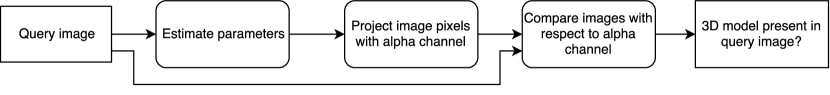
Figure 1: Data flow diagram of the triple-staged network structure for a single 3D model. The model parameters are estimated from the input image, converted back to an image and then compared to the original image.

The first stage maps the query image to a parameter vector that describes a 3D model. In our running example the parameters describe just the Euler rotation of a 3D model but in general this can also include scale, pan, and internal parameters such as dimensions, and rotational and linear joints. The estimations are clipped to their valid range. The network structure of this stage is the same as the direct classification + parameter estimation network without the task to predict the class.

The second stage of the network projects the parameter vector to a 2D image that contains the rendered 3D model in front of a black background. The alpha channel indicates to which degree each pixel belongs to the 3D model. In [5], it was shown that a deep, deconvolutional neural network can be trained to generate images that are parametrised by a broad set of classes and viewpoints. Due to our smaller set of classes and parameters, we use a downscaled variant of the 1s-S network from [5]. The first and second stage together form an autoencoder where the bottleneck contains an understandable instantiation vector of the input. This concept was already applied in the context of transforming autoencoders [9].

The final stage has to compare each projected image with the query image. Here we follow [27], which shows how to compare image patches using CNNs. We adapted the 2-channel structure to create a network that compares $10\times 10$ pixel image patches with respect to the alpha channel. This network is convoluted over the output of the second stage, giving it only local data to work with. The network was trained to emit a binary output that indicates whether the original and projected image patch should be considered equal. Fig. 2 visualises how this network works.

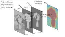
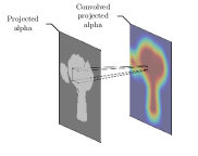
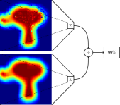
Figure 2: Visualisation of the comparison stage of the network. We convolute this stage over every $10\times 10$ pixels patch with stride 1. This generates the convoluted similarity map. Next to this similarity map, we apply a $10\times 10$ average pooling layer over the projected alpha channel to generate the convoluted, projected alpha channel. We can then directly multiply the convoluted alpha channel and the convoluted similarity map to end up with the normalized, convoluted similarity map. Next we feed both the normalized, convoluted similarity map and the convoluted, projected alpha channel, as a whole, into a single-output, sum–reduction layer. Finally we obtain the ratio by having a single output multiply the similarity sum with the reciprocal of the total weight sum. To obtain a final verdict we apply a threshold $\Theta$ over the output (cf. Section 4)

The combination of the three stages is capable of determining the presence of a single class in the query image. This does not scale well since a separate network has to be trained for each and every class. This issue is addressed by adding the class to generate as a parameter to the projection stage of the network. Each stage can now be trained on data of all the 3D models at once. The class parameter improves scalability of the triple-staged network since only one network needs to be trained for multiple classes. To generate a classification for a query image, it is provided as an input to the network multiple times with a different class parameter. If there is any class where the output of the network rises above the threshold $\Theta$, we use the class that yields the highest similarity score. Otherwise we judge that none of the classes are visible in the query image.

Similarly, an optimisation we applied is to supply the class parameter to the prediction stage of the network. We add the class as additional binary channels to the query image. Without the class information passed to this network, the network would internally need to determine which class is visible in the query image. We found that supplying the class information to the network increased the robustness of the triple-staged network. Figure 3 shows the triple-staged network architecture we used.

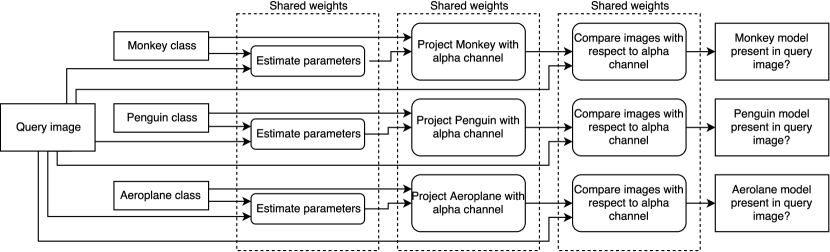
Figure 3: Architecture of our triple-staged network. Each class shares the weights in the network but hardcodes the class input parameter of the network.

2.2 Rationale

The main feature of the triple-staged architecture is to be robust against adversarial samples that cause the network to indicate that a certain class is visible when it is not. To let the neural network produce a false positive classification, an adversary needs to perturb the image such that it ultimately fools the comparator stage of the network. However, in order to do so, it must pass through both the estimator and the projector stage. Any attempt to generate a false positive will start drawing another 3D model over the existing one because the comparator compares the query image with the stable internal projection of the class in question. Ultimately then, the ‘false positive’ class will be evidently visible in the query image.

Since the comparator network directly consumes the query image, this network could still be susceptible to adversarial perturbations of the query image in much the same way as a normal classifier would be. In order to reduce susceptibility, we limited the input space of the network to a single $10\times 10$ pixel patch. This is enough to learn the general concept of two patches being “similar” (modulo some minor deviations and/or artefacts) but it is not enough to learn longer range correlations in the query image (that would give the adversarial a clear gradient to follow in generating adversarial input). We convolve this local network across the whole image, hence an adversary would need to simultaneously fool sufficiently many individual, local patch comparisons to make a significant impact on the overall similarity mass.

3 Experiment Set-up

In this section we describe how we will test the network architectures from the previous section for their robustness.

3.1 Training method

As objects to recognise, we use parametrised 3D models. We rendered $64\times 64$ pixel greyscale images of three 3D models: a Monkey (the Suzanne model from [3]), Penguin [13] and an Aeroplane [6] using Blender [3]. We took the rotation of the 3D model over three axes as our parameter space though our method is not limited to this. The rotations were uniformly sampled from the range of $[-0.5,0.5]$ radians. To give the 3D models a ‘natural’ background, we use alpha-composition to blend the 3D model in front of randomly sampled images from the ImageNet dataset [19]. This reduces overfitting of the network on the otherwise black background. We generated $4\times 10^{4}$ samples for each class. The None class simply consists of random ImageNet images.

We used Caffe [11] for the network implementations. The direct classification networks were trained using all $16\times 10^{4}$ samples. We left the predicted parameter vector for the negative samples undefined. Each stage of the triple-staged was trained separately. The estimator stage was only trained on the subset of positive samples. The second stage was trained on the original data as rendered through Blender. The input of this stage consists of the binary encoding of the class and the rotation parameters.

The data for the third stage of the network was generated by passing data through the first two stages of the network. This resulted in a new dataset with the query image, ground truth class, projected image and projected alpha mask. From this data we generated a balanced dataset where half of the samples should be considered the same and the other half of the samples is not. The samples that are considered different compare the query image, which is either a random ImageNet image or one of the 3D models in front of an ImageNet background, against one of the projected images by the second stage of the network. From this training set we sampled $10\times 10$ pixel patches where the projected alpha mask indicated that at least $1\%$ of the pixels belonged to the model. The other samples do not matter since their comparison is cancelled out by the multiplication with the projected alpha (visualised in Fig. 2).

3.2 Adversarial Image Generation

When we want to generate an adversarial query image $\tilde{x}$, we search for a minimal perturbation of the original image $x$ that is sufficient to flip the classifier towards a chosen adversarial target class value $y$. To do this we adopt the fast gradient sign method of [7]. The fast gradient sign method can efficiently generate adversarial images using backpropagation. Our aim is to generate adversarial samples that flip the classification to another positive class value $y$. Specifically, we perturb an image by computing

$$\tilde{x}=\text{clip}(x-\text{sign}({\nabla}_{x}J(\theta,x,y)),0,255),$$

with $J$ the loss function over the query image $x$ and network parameters $\theta$. Since we use 8-bit greyscale images with a range of $[0,255]$, each pixel of the image will be minimally perturbed. This function is applied as often as needed to flip the classification of the network to the target $y$.

4 Results

We test our networks on a separate test set which consists of 10000 samples of each class. The backgrounds are sourced from the ImageNet validation set. We first measure the classification performance of the networks on non-adversarial images, see Table 1 for the results. The direct classification networks have the lowest error rate, followed by the triple-staged network. With $\Theta=0.2$ or $\Theta=0.7$, the ‘None’ class is chosen more/less often. Although choosing $\Theta$ somewhere in the middle seems to be the best option purely in terms of minimizing classification error, our data clearly shows that there is a trade-off to consider concerning robustness to adversarial samples versus classification error.

Table 1: Classification error rate of the networks.

Network	Error rate
Direct classification	$0.01\%$
Direct classification + Parameter Estimation	$0.01\%$
Triple-staged, $\Theta=0.2$	$1.34\%$
Triple-staged, $\Theta=0.45$	$0.57\%$
Triple-staged, $\Theta=0.7$	$3.09\%$

To compare the networks under adversarial conditions, we measure how many iterations of adversarial perturbation it takes to change the classification and how much the image was changed. Here we follow [23] who measure the amount of perturbation in adversarial sample for original sample as distortion which is defined as:

$$\frac{1}{255}\sqrt{\frac{\sum_{i}{(\tilde{x}_{i}-x_{i})}^{2}}{n}},$$

where $x$ is the original image, $\tilde{x}$ is the distorted image and $n$ is the number of pixels.

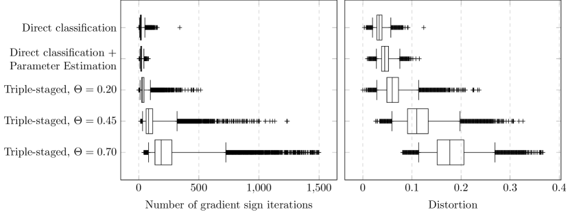
Figure 4: The effort required to convert the test images that contain one of the 3D models to an image where the network judges that another class of the 3D models is visible. There were no cases with 0 steps. For readability we clipped the number of steps in the graph to a maximum of 1500. The whiskers are placed at the 2^nd and 98^th percentile.

We performed experiments with both false positive and false negative adversarial images. To generate a false positive adversarial image, we start from a test image containing one of our 3D objects, say a Monkey. Following the procedure explained in Section 3.2, we then construct an adversarial image that makes the network believe that the image belongs to the other class, once for a Penguin and once for an Aeroplane. We repeat this procedure for all test images. Figure 4 shows the results for the false positive adversarial images. The figure shows that for the direct classification networks the required changes are limited: the median of their distortion is still below $0.1$ which indicates that the adversarial image is still very similar to the original one. The examples in Fig. 5a show this. In contrast, the triple-staged network requires significantly more effort to change the classification. The higher the threshold, the more the query image needs to look like the internally projected image. Figure 5b shows false positive adversarial samples for the $\Theta=0.70$ network. The triple-staged network structure requires the adversary to generate images that really start to look like the adversary class. As Table 1 shows, the error rate on normal samples is still reasonable at this threshold.

(a)

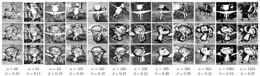
(b)

Figure 5: Generated adversarial images, ordered by distortion. The top row contains the original image, the second row the adversarial variant. The bottom row contains the original image with the Monkey 3D model alpha-blended, rendered by Blender using the predicted parameters. Every column is annotated with the distortion $d$ and number of iterations $n$. All adversarial samples are classified as the Monkey class.

When we generate false positives, we start with an image that contains one of the classes and perturb it to an image that is classified as ‘None’. For the direct classification networks this is the 4^th class they can predict. In the case of the triple-staged network, the output for every class has to be below the threshold $\Theta$. Figure 6 shows that the number of required iterations is significantly higher for $\Theta=0.20$ compared to the other networks. Note that in contrast to the false positives, the false negative adversarial samples are better resisted using a lower threshold. By lowering the threshold, the triple-staged network is less likely to switch to the ‘None’ class, requiring more work from the adversary.

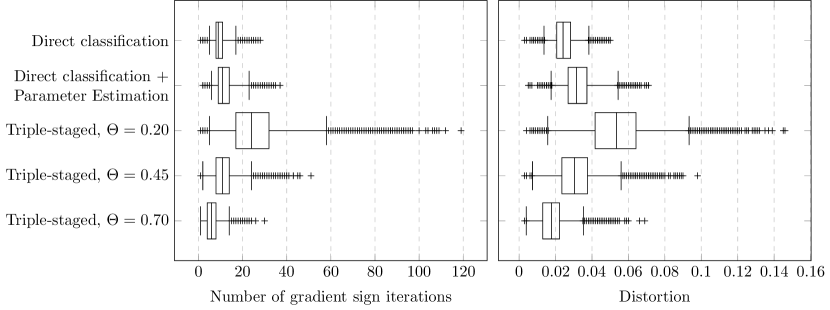
Figure 6: The effort required to convert the test images that contain one of the 3D models to an image where the network judges that none of the 3D models is visible. This was possible for all the samples in the test set. The instances that were misclassified in the first place were filtered out. This is $0.00\%,0.01\%,0.17\%,0.77\%,4.12\%$ of the data respectively from top to bottom. The whiskers are placed at the 2^nd and 98^th percentile.

5 Discussion

We have adapted the classical network structure for classifier tasks and shown significant improvements in robustness against adversarial samples. In order not to pollute the results we have not taken into account other types of solutions against adversarial samples such as adversarial training. This does not however mean these techniques would not be useful also in our setting. As future work we therefore plan to incorporate adversarial training into our approach.

Future work could also apply our technique to include more parameters including internal deformations, using joints etc. We have only tested three 3D models with a limited parameter space. In [15, 21] it was already shown that it is possible to estimate viewpoints of 3D models in real-world images. Dosovitskiy et al. [5] have shown that a deconvolutional neural can generate images based on many classes and viewpoints. This opens up possibilities to expand our work to a real-world situation.

For the present work we opted to train the network in three separate stages. This allowed us quite a bit of control over the network architecture which, in turn, allowed us a shorter route to testing the working hypothesis. Nevertheless, as future work, it would be interesting to develop end-to-end training methods for which the architecture would be more emergent and less explicit. As an obvious first step we could conceive of training the first two stages end-to-end, as an autoencoder, instead of using manually parameterized 3D models.

References

- [1] Aubry, M., Maturana, D., Efros, A., Russell, B., Sivic, J.: Seeing 3d chairs: exemplar part-based 2d-3d alignment using a large dataset of cad models. In: CVPR (2014), http://www.di.ens.fr/willow/research/seeing3Dchairs/
- [2] Berntsen, H.: Adversarial background augmentation improves object localisation using convolutional neural networks. Master’s thesis, Radboud University (2015), http://www.ru.nl/publish/pages/769526/z_thesis_harm_berntsen.pdf
- [3] Blender Online Community: Blender - a 3D modelling and rendering package. Blender Foundation, Blender Institute, Amsterdam (2015), http://www.blender.org
- [4] Chalupka, K., Perona, P., Eberhardt, F.: Visual causal feature learning. In: UAI (2015), http://auai.org/uai2015/proceedings/papers/109.pdf
- [5] Dosovitskiy, A., Springenberg, J.T., Tatarchenko, M., Brox, T.: Learning to generate chairs, tables and cars with convolutional neural networks. CoRR (2015), http://arxiv.org/abs/1411.5928v3
- [6] Fraga, P.: Antonov an - 71 - 3d model - .obj, .mb (2015), http://tf3dm.com/3d-model/antonov-an-71-no-texture-77342.html
- [7] Goodfellow, I.J., Shlens, J., Szegedy, C.: Explaining and harnessing adversarial examples. CoRR (2015), http://arxiv.org/abs/1412.6572
- [8] Gu, S., Rigazio, L.: Towards deep neural network architectures robust to adversarial examples. CoRR (2014), http://arxiv.org/abs/1412.5068v4
- [9] Hinton, G.E., Krizhevsky, A., Wang, S.D.: Transforming auto-encoders. In: ICANN (2011)
- [10] Huang, R., Xu, B., Schuurmans, D., ri, C.S.: Learning with a strong adversary. CoRR (2015), http://arxiv.org/abs/1511.03034
- [11] Jia, Y., Shelhamer, E., Donahue, J., Karayev, S., Long, J., Girshick, R., Guadarrama, S., Darrell, T.: Caffe: Convolutional architecture for fast feature embedding. CoRR (2014), http://arxiv.org/abs/1408.5093
- [12] Krizhevsky, A., Sutskever, I., Hinton, G.E.: Imagenet classification with deep convolutional neural networks. In: Pereira, F., Burges, C.J.C., Bottou, L., Weinberger, K.Q. (eds.) Advances in Neural Information Processing Systems 25, pp. 1097–1105. Curran Associates, Inc. (2012), http://papers.nips.cc/paper/4824-imagenet-classification-with-deep-convolutional-neural-networks.pdf
- [13] Legaz, K.: Tux (armatured) - 3d models - kator legaz (2015), http://web.archive.org/web/20151014015438/http://www.katorlegaz.com/3d_models/miscellaneous/0167/index.php
- [14] Lyu, C., Huang, K., Liang, H.N.: A unified gradient regularization family for adversarial examples. In: ICDM (2015), http://arxiv.org/abs/1511.06385
- [15] Massa, F., Russell, B.C., Aubry, M.: Deep exemplar 2d-3d detection by adapting from real to rendered views. CoRR (2015), http://arxiv.org/abs/1512.02497
- [16] Nguyen, A., Yosinski, J., Clune, J.: Deep neural networks are easily fooled: High confidence predictions for unrecognizable images. In: Computer Vision and Pattern Recognition (CVPR), 2015 IEEE Conference on. IEEE (2015), http://www.evolvingai.org/fooling
- [17] Norouzi, M., Mikolov, T., Bengio, S., Singer, Y., Shlens, J., Frome, A., Corrado, G., Dean, J.: Zero-shot learning by convex combination of semantic embeddings. In: International Conference on Learning Representations (2014), http://arxiv.org/abs/1312.5650
- [18] Peng, X., Sun, B., Ali, K., Saenko, K.: Learning deep object detectors from 3d models. In: ICCV (2015), http://www.cv-foundation.org/openaccess/content_iccv_2015/html/Peng_Learning_Deep_Object_ICCV_2015_paper.html
- [19] Russakovsky, O., Deng, J., Su, H., Krause, J., Satheesh, S., Ma, S., Huang, Z., Karpathy, A., Khosla, A., Bernstein, M., Berg, A.C., Fei-Fei, L.: ImageNet Large Scale Visual Recognition Challenge. International Journal of Computer Vision (IJCV) 115(3), 211–252 (2015), http://arxiv.org/abs/1409.0575
- [20] Simonyan, K., Vedaldi, A., Zisserman, A.: Deep inside convolutional networks: Visualising image classification models and saliency maps. In: Workshop at International Conference on Learning Representations (2014), http://arxiv.org/abs/1312.6034
- [21] Su, H., Qi, C.R., Li, Y., Guibas, L.J.: Render for cnn: Viewpoint estimation in images using cnns trained with rendered 3d model views. In: The IEEE International Conference on Computer Vision (ICCV) (2015), http://arxiv.org/abs/1505.05641
- [22] Sun, B., Saenko, K.: From Virtual to Reality: Fast Adaptation of Virtual Object Detectors to Real Domains. In: Proceedings of the British Machine Vision Conference. BMVA Press (2014), http://www.bmva.org/bmvc/2014/papers/paper062/index.html
- [23] Szegedy, C., Zaremba, W., Sutskever, I., Bruna, J., Erhan, D., Goodfellow, I., Fergus, R.: Intriguing properties of neural networks. In: International Conference on Learning Representations (2014), http://research.google.com/pubs/pub42503.html
- [24] Tabacof, P., Valle, E.: Exploring the space of adversarial images. CoRR (2015), http://arxiv.org/abs/1510.05328
- [25] Tang, K.D., Paluri, M., Fei-Fei, L., Fergus, R., Bourdev, L.D.: Improving image classification with location context. In: ICCV (2015), http://www.cv-foundation.org/openaccess/content_iccv_2015/papers/Tang_Improving_Image_Classification_ICCV_2015_paper.pdf
- [26] Ullman, S., Assif, L., Fetaya, E., Harari, D.: Atoms of recognition in human and computer vision. Proceedings of the National Academy of Sciences (2016), http://www.pnas.org/content/early/2016/02/09/1513198113
- [27] Zagoruyko, S., Komodakis, N.: Learning to compare image patches via convolutional neural networks. In: The IEEE Conference on Computer Vision and Pattern Recognition (CVPR) (2015), http://www.cv-foundation.org/openaccess/content_cvpr_2015/papers/Zagoruyko_Learning_to_Compare_2015_CVPR_paper.pdf