Heavy quark potential with hyperscaling violation

Abstract

In this paper, we investigate the behavior of the heavy quark potential in the backgrounds with hyperscaling violation. The metrics are covariant under a generalized Lifshitz scaling symmetry with the dynamical Lifshitz parameter $z$ and hyperscaling violation exponent $\theta$. We calculate the potential for a certain range of $z$ and $\theta$ and discuss how it changes in the presence of the two parameters. Moreover, we add a constant electric field to the backgrounds and study its effects on the potential. It is shown that the heavy quark potential depends on the non-relativistic parameters. Also, the presence of the constant electric field tends to increase the potential.

I Introduction

AdS/CFT Maldacena:1997re ; Gubser:1998bc ; MadalcenaReview , which relates a d-dimensional quantum field theory with its dual gravitational theory, living in(d+1) dimensions, has yielded many important insights into the dynamics of strongly-coupled gauge theories. For reviews, see Refs CP ; CP1 ; MA ; SS ; EC ; JS ; KB ; MC ; TM ; RG ; MA1 ; UG and references therein.

Due to the broad application of this characteristic, many authors have considered the generalizations of the metrics that dual to field theories. One of such generalizations is to use metric with hyperscaling violation. Usually, the metric is considered to be an extension of the Lifshitz metric and has a generic Lorentz violating form TA ; KBA ; HS ; KN ; FD . As we know, Lorentz symmetry represents a foundation of both general relativity and the standard model, so one may expect new physics from Lorentz invariance violation. For that reason, the metrics with hyperscaling violation have been used to describe the string theory BG ; EP ; MA2 ; JSA ; EK , holographic superconductors EBR ; SJS ; YYB ; QYP as well as QCD JSA1 ; JSA2 ; KBI .

The heavy quark potential of QCD is an important quantity that can probe the confinement mechanism in the hadronic phase and the meson melting in the plasma phase. In addition, it has been measured in great detail in lattice simulations. The heavy quark potential for $\mathcal{N}=4$ SYM theory was first obtained by Maldacena in his seminal work Maldacena:1998im . Interestingly, it is shown that for the $AdS_{5}$ space the energy shows a purely Coulombian behavior which agrees with a conformal gauge theory. This proposal has attracted lots of interest. After Maldacena:1998im , there are many attempts to address the heavy quark potential from the holography. For example, the potential at finite temperature has been studied in AB ; SJ . The sub-leading order correction to this quantity is discussed in SX ; ZQ . The potential has also been investigated in some AdS/QCD models OA2 ; SH1 . Other important results can be found, for example, in JG ; FB ; LM ; YK ; SH .

Although the theories with hyperscaling violation are intrisically non-relativistic, we can use them as toy models for quarks from the holography point of view. In addition, one can expect the results that obtained from these theories shed qualitative insights into analogous questions in QCD. In this paper, we will investigate the heavy quark potential in the Lifshitz backgrounds with hyperscaling violation. We want to know what will happen to the potential if we have the quark anti-quark pair in such backgrounds? More specifically, we would like to see how the potential changes in the presence of the non-relativistic parameters. In addition, we will add a constant electric field to the backgrounds and study how it affects the potential. These are the main motivations of the present work.

We organize the paper as follows. In the next section, the backgrounds of the hyperscaling violation theories in EK are briefly reviewed. In section 3, we study the heavy quark potential in these backgrounds in terms of the $z$ and $\theta$ parameters. In section 4, we investigate a constant electric field effect on the heavy quark potential. The last part is devoted to conclusion and discussion.

II hyperscaling violation theories

Let us begin with a brief review of the background in EK . It has been argued that the Lorentz invariance is broken in this background metric. Although charge densities induce a trivial (gapped) behavior at low energy/temperature, there still exist special cases where there are non-trivial IR fixed points (quantum critical points) where the theory is scale invariant. Usually, the metric is expressed as BG

$$ds^{2}=u^{\theta}[-\frac{dt^{2}}{u^{2z}}+\frac{b_{0}du^{2}+dx^{i}dx^{i}}{u^{2}}],$$ (1)

where $b_{0}=\ell^{2}$ with $\ell$ the IR scale. The above metric is covariant under a generalized Lifshitz scaling symmetry, that is

$$t\rightarrow\lambda^{z}t,\qquad u\rightarrow\lambda u,\qquad x^{i}\rightarrow\lambda x^{i},\qquad ds^{2}\rightarrow\lambda^{-\theta}ds^{2},$$ (2)

where z is called the dynamical Lifshitz parameter or the dynamical critical exponent which characterizes the behavior of system near the phase transition. $\theta$ stands for the hyperscaling violation exponent which is responsible for the non-stand scaling of physical quantities as well as controls the transformation of the metric. The scalar curvature of these geometries is

$$R=-\frac{3\theta^{2}-4(z+3)\theta+2(z^{2}+3z+6)}{b_{0}}u^{-\theta}.$$ (3)

The geometries are flat when $\theta=2$, $z=0,1$. The geometry is Ricci flat when $\theta=4$, $z=3$. The geometry is in Ridler coordinates when $\theta=0$ and $z=1$. Usually, the above special solutions violate the Gubser bound conditions EK . In addition, the pure Lifshitz case is related to $\theta=0$.

By using a radical redefinition

$$u=(2-z)r^{\frac{1}{2-z}},$$ (4)

and rescaling t and $x^{i}$, we have the following metric

$$ds^{2}\sim r^{\frac{\theta-2}{2-z}}[-f(r)dt^{2}+\frac{dr^{2}}{f(r)}+dx^{i}dx^{i}],\qquad f(r)=f_{0}r^{\frac{2(1-z)}{2-z}},$$ (5)

with $f_{0}=(2-z)^{2(1-z)}$.

In the presence of hyperscaling violations, the energy scale is

$$E\simeq u^{\frac{\theta-2z}{2}}\simeq r^{\frac{\theta-2z}{2(2-z)}}.$$ (6)

For the generalized scaling solutions of Eq.(5), the Gubser bound conditions are as follows:

$$\frac{2z+3(2-\theta)}{2(z-1)-\theta}>0,\qquad\frac{z-1}{2(z-1)-\theta}>0,\qquad\frac{2(z-1)+3(2-\theta)}{2(z-1)-\theta}>0.$$ (7)

Also, to consider the thermodynamic stability, one needs

$$\frac{z}{2(z-1)-\theta}>0.$$ (8)

More discussions about other generalized Lifshitz geometries can be found in EK .

The generalizations of Eq.(5) to include finite temperature can be written as

$$ds^{2}\sim(\frac{r}{\ell})^{-\alpha}[-f(r)dt^{2}+\frac{dr^{2}}{f(r)}+dx^{i}dx^{i}],\qquad f(r)=f_{0}(\frac{r}{\ell})^{2\beta}h,\qquad h=1-(\frac{r}{r_{h}})^{\gamma}.$$ (9)

where $\alpha=\frac{\theta-2}{z-2}$, $\beta=\frac{z-1}{z-2}$, $\gamma=\frac{2z+3(2-\theta)}{2(2-z)}$.

The Hawking temperature is

$$T=\frac{f_{0}}{8\pi\ell}(\frac{r_{h}}{\ell})^{\frac{z}{z-2}}|\frac{2z-3\theta+6}{z-2}|.$$ (10)

III heavy quark potential

In the holographic description, the heavy quark potential is given by the expectation value of the static Wilson loop

$$W(C)=\frac{1}{N}TrPe^{i\int A_{\mu}dx^{\mu}},$$ (11)

where C is a closed loop in a 4-dimensional space time and the trace is over the fundamental representation of the SU(N) group. $A_{\mu}$ is the gauge potential and $P$ enforces the path ordering along the loop $C$. The heavy quark potential can be extracted from the expectation value of this rectangular Wilson loop in the limit $\mathcal{T}\rightarrow\infty$,

$$<W(C)>\sim e^{-\mathcal{T}V}.$$ (12)

On the other hand, the expectation value of Wilson loop in (12) is given by

$$<W(C)>\sim e^{-S_{c}},$$ (13)

where $S_{c}$ is the regularized action. Therefore, the heavy quark potential can be expressed as

$$V=\frac{S_{c}}{\mathcal{T}}.$$ (14)

We now analyze the heavy quark potential using the metric of Eq.(9). The string action can reduce to the Nambu-Goto action

$$S=-\frac{1}{2\pi\alpha^{\prime}}\int d\tau d\sigma\sqrt{-detg_{\alpha\beta}},$$ (15)

where $g$ is the determinant of the induced metric on the string world sheet embedded in the target space, i.e.

$$g_{\alpha\beta}=G_{\mu\nu}\frac{\partial X^{\mu}}{\partial\sigma^{\alpha}}\frac{\partial X^{\nu}}{\partial\sigma^{\beta}},$$ (16)

where $X^{\mu}$ and $G_{\mu\nu}$ are the target space coordinates and the metric, and $\sigma^{\alpha}$ with $\alpha=0,1$ parameterize the world sheet.

Using the parametrization $X^{\mu}=(t,x,0,0,r)$, $\sigma=x$, $\tau=t$ and $r=r(x)$, we extremize the open string worldsheet attached to a static quark at $x=+L/2$ and an anti-quark at $x=-L/2$. Then the induced metric of the fundamental string is given by

$$g_{\alpha\beta}=b(r)\left(\begin{array}[]{cc}-f(r)&0\\ 0&1+\frac{\dot{r}^{2}}{f(r)}\end{array}\right),$$ (17)

with $b(r)=(\frac{r}{\ell})^{-\alpha}$, $\dot{r}=\frac{dr}{dx}$.

Plugging (17) into (15), the Euclidean version of Nambu-Goto action in Eq.(9) becomes

$$S=\frac{\mathcal{T}}{2\pi\alpha^{\prime}}\int dx\sqrt{b^{2}(r)[f(r)+\dot{r}^{2}]}.$$ (18)

We now identify the Lagrangian as

$$\mathcal{L}=\sqrt{b^{2}(r)[f(r)+\dot{r}^{2}]}.$$ (19)

Note that $\mathcal{L}$ does not depend on $x$ explicitly, so the corresponding Hamiltonian will be a constant of motion, ie.,

$$H=\frac{\partial\mathcal{L}}{\partial\dot{r}}\dot{r}-\mathcal{L}=Constant=C.$$ (20)

This constant can be found at special point $r(0)=r_{c}$, where $r_{c}^{\prime}=0$, as

$$H=-\sqrt{f(r_{c})b^{2}(r_{c})},$$ (21)

then a differential equation is derived,

$$\dot{r}=\sqrt{\frac{f^{2}(r)b^{2}(r)-f(r)f(r_{c})b^{2}(r_{c})}{f(r_{c})b^{2}(r_{c})}}.$$ (22)

with

$$f(r_{c})=f_{0}(\frac{r_{c}}{\ell})^{2\beta}h_{1},\qquad h_{1}=1-(\frac{r_{c}}{r_{h}})^{\gamma},\qquad b(r_{c})=(\frac{r_{c}}{\ell})^{-\alpha}.$$ (23)

By integrating (22) the separation length $L(\theta,z)$ of quark-antiquark pair becomes

$$L(\theta,z)=2\int_{0}^{r_{c}}dr\sqrt{\frac{f(r_{c})b^{2}(r_{c})}{f^{2}(r)b^{2}(r)-f(r)f(r_{c})b^{2}(r_{c})}}.$$ (24)

On the other hand, plugging (22) into the Nambu-Goto action of Eq.(18), one finds the action of the heavy quark pair

$$S=\frac{\mathcal{T}}{\pi\alpha^{\prime}}\int_{0}^{r_{c}}drb^{2}(r)\sqrt{\frac{f(r)}{f(r)b^{2}(r)-f(r_{c})b^{2}(r_{c})}}.$$ (25)

This action is divergent, but the divergences can be avoided by subtracting the inertial mass of two free quarks, which is given by

$$S_{0}=\frac{\mathcal{T}}{\pi\alpha^{\prime}}\int_{0}^{r_{h}}drb(r).$$ (26)

Subtracting this self-energy, the regularized action is obtained:

$$S_{c}=S-S_{0}.$$ (27)

Applying (14), we end up with the heavy quark potential with hyperscaling violation

$$V(\theta,z)=\frac{1}{\pi\alpha^{\prime}}\int_{0}^{r_{c}}dr[b^{2}(r)\sqrt{\frac{f(r)}{f(r)b^{2}(r)-f(r_{c})b^{2}(r_{c})}}-b(r)]-\frac{1}{\pi\alpha^{\prime}}\int_{r_{c}}^{r_{h}}drb(r),$$ (28)

Note that the potential V(z) in the Lifshitz spacetime UH ; JK can be derived from (28) if we neglect the effect of the hyperscaling violation exponent by plugging $\theta=0$ in (28). Also, in the limit ($\theta=0,z=1$), the Eq.(28) can reduce to the finite temperature case in AB ; SJ .

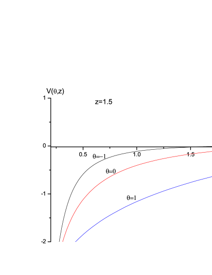
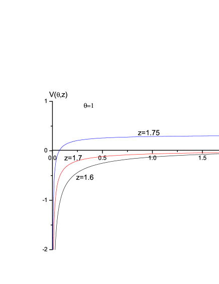
Figure 1: Plots of $V(\theta,z)$ versus $L(\theta,z)$. Left: $z=1.5$, from top to bottom $\theta=-1,0,1$ respectively; Right: $\theta=1$, from top to bottom $z=1.75,1.7,1.6$ respectively.

Before evaluating the heavy quark potential of Eq.(28), we should pause here to determine the allowed region for z and $\theta$ at hand. The space boundary is considered at $r=0$, consequently $\alpha>0$. To avoid the Eq.(28) being ill-defined, it is required that $\gamma>0$. Moreover, one should consider the Gubser conditions of (7) and the thermodynamic stability condition of (8). With these restrictions, one finds

$$1<z<2,\qquad\theta<2,\qquad\theta<z,$$ (29)

then one can choose the values of z and $\theta$ in such a range.

In Fig.1, we plot the potential $V(\theta,z)$ versus distance $L(\theta,z)$ with different z, $\theta$. In the left plots, the dynamical exponent is $z=1.5$ and from top to bottom the hyperscaling violation exponent is $\theta=-1,0,1$, respectively. In the right plots, $\theta=1$ and from top to bottom $z=1.75,1.7,1.6$, respectively. From the figures, we can see clearly that by increasing $\theta$ the potential decreases. One finds also that increasing $z$ leads to increasing the potential. In other words, increasing z and $\theta$ have different effects on the potential. Then one can change the potential by changing the values of these parameters. Therefore, the heavy quark potential depends on the non-relativistic parameters.

To study how the potential changes with the temperature T, we show $V(\theta,z)$ as a function of $L(\theta,z)$ with $z=1.6,\theta=1$ in Fig.2. From Eq.(10), we can see that T is a decreasing function of $z_{h}$ for $z=1.6$. So one finds in Fig.2 that increasing T (or decreasing $z_{h}$) leads to increasing the potential. This result is consistently with the finding of AB ; SJ .

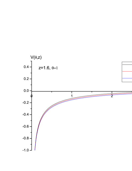
Figure 2: Plots of $V(\theta,z)$ versus $L(\theta,z)$ with $z=1.6,\theta=1$. From top to bottom $r_{h}=3.2,3.5,3.8$ respectively.

Moreover, to see the short distance behavior of the potential, we take the limit $L(\theta,z)T\rightarrow 0$ and find the following approximate formula

$$L(\theta,z)\simeq\frac{2f_{0}^{-1/2}}{\alpha-2\beta+1}r_{c}^{1-\beta},\qquad V(\theta,z)\simeq\frac{\sqrt{\lambda}}{\pi(1-\alpha)}r_{c}^{1-\alpha},$$ (30)

which yields

$$V(\theta,z)\propto L(\theta,z)^{\theta-z}.$$ (31)

One can see that the potential is dependent on $z$ and $\theta$. In the special case of $\theta=0,z=1$ (or $\alpha=2,\beta=0$), one finds that the potential is of Coulomb type:

$$V(\theta,z)\simeq-\frac{\sqrt{\lambda}}{1.5\pi L(\theta,z)},$$ (32)

but for other cases, the potential may not be Coulombian.

IV Effect of constant electric field

In this section, we study the effect of a constant electric field on the heavy quark potential following the method proposed in TM . The constant B-field is along the $x^{1}$ and $x^{2}$ directions. As the field strength is involved in the equations of motion, this ansatz could be a good solution to supergravity as well as a simple way of studying the B-field correction. The constant B-field is added to the metric of Eq.(9) by the following form:

$$B=B_{01}dt\wedge dx^{1}+B_{12}dx^{1}\wedge dx^{2},$$ (33)

where $B_{01}$ and $B_{12}$ are assumed to be constants with $B_{01}=E$ the NS-NS antisymmetric electric field and $B_{12}=H$ the NS-NS antisymmetric magnetic field.

The constant B-field considered here is only turned on $x^{1}$ direction, which implies $H=0$. After adding an electric field to this background metric of Eq.(9), the string action is given by

$$S=-\frac{1}{2\pi\alpha^{\prime}}\int d\tau d\sigma\sqrt{-det(g+b)_{\alpha\beta}},$$ (34)

where $g_{\alpha\beta}$ is given in Eq.(17). $b_{\alpha\beta}=B_{\mu\nu}\partial_{\alpha}X^{\mu}\partial_{\beta}X^{\nu}$, is obtained as

$$b_{\alpha\beta}=\left(\begin{array}[]{cc}0&0\\ 0&\xi\end{array}\right),$$ (35)

then the string action in Eq.(34) reads

$$S=\frac{\mathcal{T}}{2\pi\alpha^{\prime}}\int dx\sqrt{b^{2}(r)f(r)+b(r)f(r)\xi+b^{2}(r)\dot{r}^{2}}.$$ (36)

Parallel to the case of the previous section, we have

$$\dot{r}=\sqrt{\frac{A^{2}(r)-A(r)A(r_{c})}{A(r_{c})b^{2}(r)}}.$$ (37)

with

$$A(r)=b^{2}(r)f(r)+b(r)f(r)\xi,\qquad A(r_{c})=b^{2}(r_{c})f(r_{c})+b(r_{c})f(r_{c})\xi.$$ (38)

We call again the separation length and the heavy quark potential as $L$ and $V$, respectively. One finds

$$L=2\int_{0}^{r_{c}}dr\sqrt{\frac{A(r_{c})b^{2}(r)}{A^{2}(r)-A(r)A(r_{c})}},$$ (39)

and

$$V=\frac{1}{\pi\alpha^{\prime}}\int_{0}^{r_{c}}dr[\sqrt{\frac{A(r)b^{2}(r)}{A(r)-A(r_{c})}}-b(r)]-\frac{1}{\pi\alpha^{\prime}}\int_{r_{c}}^{r_{h}}drb(r).$$ (40)

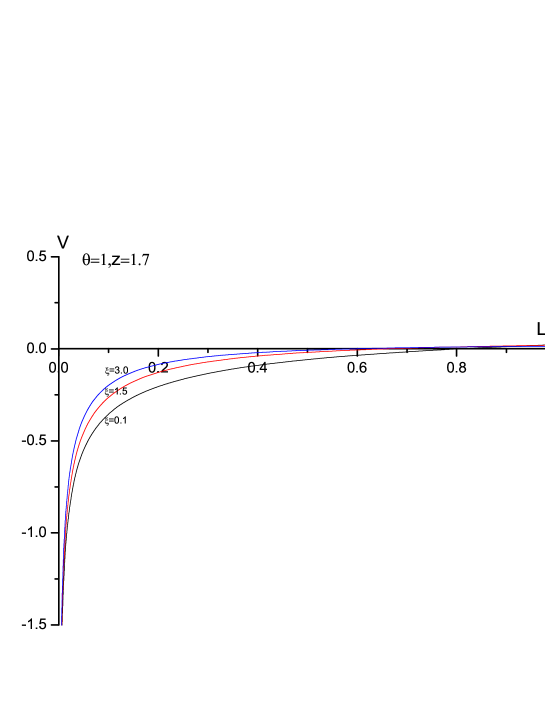
Figure 3: Plots of $V$ versus $L$ with different $\xi$. Here $z=1.7$, $\theta=1$. From top to bottom $\xi=3.0,1.5,0.1$.

To see the effect of the constant electric field $\xi$ on the heavy quark potential in the backgrounds with hyperscaling violation. We plot the heavy quark potential as a function of the inter distance for $z=1.7$, $\theta=1$ with three different $\xi$ in Fig.3. In the plots from top to bottom $\xi=3.0,1.5,0.1$ respectively. From the figures, we can see that the heavy quark potential increases with increasing $\xi$. In other words, the presence of the constant electric field leads to a smaller screening radius. This result can be understood by considering the relation between the potential and the viscosity of the medium. It was argued JN that increasing the viscosity, the screening of the potential due to the thermal medium weakens and so the potential decreases. On the other hand, the presence of the constant electric field tends to weaken the viscosity TM . Thus, increasing the constant electric field leads to weakening the viscosity or increasing the potential.

V conclusion and discussion

In this paper, we have investigated the heavy quark potential in the backgrounds with hyperscaling violation at finite temperature. These theories are strongly coupled with anisotropic scaling symmetry in the time and a spatial direction. Although the theories are not directly applicable to QCD, the features of them are similar to QCD. Therefore one can expect the results that obtained from these theories shed qualitative insights into analogous questions in QCD. In addition, an understanding of how the heavy quark potential changes by these theories may be useful for theoretical predictions.

In section 3, we used the holographic description to calculate the heavy quark potential at finite temperature. We considered the space boundary at $r=0$ and discussed the potential for a certain range of $z$ and $\theta$ which satisfies the Gubser conditions and the thermodynamic stability condition. In is shown that increasing z and $\theta$ have different effects: the potential increases as z increases but it decreases as $\theta$ increases. As a result, the heavy quark potential depends on the non-relativistic parameters. In section 4, we added a constant electric field to the background metrics and study its effect on the heavy quark potential. We observed that the potential rises as the constant electric field increases. In other words, the presence of the constant electric field leads to increasing the heavy quark potential.

Finally, it is interesting to mention that the drag force CP can also be studied in the backgrounds with hyperscaling violation. We will leave this for further study.

VI Acknowledgments

This research is partly supported by the Ministry of Science and Technology of China (MSTC) under the 973 Project no. 2015CB856904(4). Zi-qiang Zhang and Gang Chen are supported by the NSFC under Grant no. 11475149. De-fu Hou is supported by the NSFC under Grant no. 11375070, 11521064.

References

- (1) J. M. Maldacena, Adv. Theor. Math. Phys. 2, 231 (1998) Int. J. Theor. Phys. 38, 1113 (1999).
- (2) S. S. Gubser, I. R. Klebanov and A. M. Polyakov, Phys. Lett. B428, 105 (1998).
- (3) O. Aharony, S. S. Gubser, J. Maldacena, H. Ooguri and Y. Oz, Phys. Rept. 323, 183 (2000).
- (4) C. P. Herzog, A. Karch, P. Kovtun, C. Kozcaz and L. G. Yaffe, JHEP 0607 (2006) 013.
- (5) C. P. Herzog, JHEP 09 (2006) 032.
- (6) M. Ali-Akbari, U. Gursoy, JHEP 01 (2012) 105.
- (7) S. S. Gubser, Phys. Rev. D 74 126005 (2006).
- (8) E. Caceres and A. Guijosa, JHEP11 (2006) 077.
- (9) J. Sadeghi and B. Pourhassan, JHEP 12 (2008) 026.
- (10) K. Bitaghsir Fadafana, H. Soltanpanahi, JHEP 01 (2012) 085.
- (11) M. Chernicoff, J. A. Garcia and A. Guijosa, JHEP 09 (2006) 068.
- (12) T. Matsuo, D. Tomino and W. Y. Wen, JHEP 10 (2006) 055.
- (13) R-G. Cai, S. Chakrabortty, S. He, L. Li, JHEP02 (2013) 068.
- (14) M. Ali-Akbari M and K. B. Fadafan, Nucl.Phys.B 835 221 (2010).
- (15) U. Gursoy and E. Kiritsis, JHEP 0802 (2008) 032.
- (16) T. Azeyanagi, W. Li, and T. Takayanagi, JHEP 0906 (2009) 084.
- (17) K. Balasubramanian and K. Narayan, JHEP 1008 (2010) 014 032.
- (18) H. Singh, JHEP 1207 082 (2012).
- (19) K. Narayan, Phys. Rev. D 85, 106006 (2012).
- (20) P. Dey and S. Roy, Phys. Rev. D 86, 066009 (2012).
- (21) B. Gouteraux and E. Kiritsis, JHEP 1112, 036 (2011).
- (22) E. Perlmutter, JHEP 1102, 013 (2011).
- (23) M. Alishahiha and H. Yavartanoo, JHEP 1211 (2012) 034.
- (24) J. Sadeghi, B. Pourhasan, and F. Pourasadollah, Phys. Lett. B 720 244 (2013).
- (25) E. Kiritsis, JHEP 1301 (2013) 030.
- (26) E. Brynjolfsson, U.H.Danielsson, L.Thorlacius, T.Zingg, J.Phys. A 43, 065401 (2010).
- (27) S.-j. Sin, S.-s. Xu, Y. Zhou, Int. J. Mod. Phys. A 26, 4617 (2011).
- (28) Y. Y. Bu, Phys. Rev. D 86, 046007 (2012)
- (29) Q.-u. Pan, S.-J. Zhang, Eur. Phys. J. C 76, 126 (2016).
- (30) J. Sadeghi and S. Heshmatian, Eur. Phys. J. C (2014) 74 3032.
- (31) J. Sadeghi and S. Heshmatian, [hep-th/1509.01309].
- (32) K. B. Fadafan and F. Saiedi, [hep-th/1504.02432].
- (33) J. M. Maldacena, Phys. Rev. Lett 80, 4859 (1998).
- (34) U. H. Danielsson and L. Thorlacius, JHEP 0903 (2009) 070 [hep-th/0812.5088]
- (35) J. Kluson, Phys. Rev. D 81 (2010) 106006.
- (36) A. Brandhuber, N. Itzhaki, J. Sonnenschein and S. Yankielowicz, Phys. Lett. B 434, 36 (1998).
- (37) S. J. Rey, S. Theisen and J. T. Yee, Nucl. Phys. B 527, 171 (1998).
- (38) S.-x. Chu, D. Hou and H.-c. Ren, JHEP 08, 004 (2009).
- (39) Z.-q. Zhang, D. Hou, H.-c Ren and L. Yin, JHEP 1107 035 (2011).
- (40) O. Andreev and V. I. Zakharov, JHEP 0704 100 (2007).
- (41) S. He, M. Huang, Q.-s. Yan, Phys. Rev. D 83 045034 (2011).
- (42) J. Greensite and P. Olesen, JHEP 9808, 009 (1998).
- (43) F. Bigazzi, A. L. Cotrone, L. Martucci and L. A. Pando Zayas, Phys. Rev. D 71, 066002 (2005).
- (44) L. Martucci, Fortsch. Phys. 53, 936 (2005).
- (45) Y. Kinar, E. Schreiber and J. Sonnenschein, Nucl. Phys. B 566, 103 (2000).
- (46) S. He, M. Huang, Q.-s. Yan, Prog. Theor. Phys. Suppl 186 504 (2010).
- (47) R. Rougemont, R. Critelli, and J. Noronha, Phys. Rev. D 91, 066001 (2015).
- (48) J. Noronha, A. Dumitru, Phys. Rev. D 91, 066001 (2015).