Efficient Reduced-Rank DOA Estimation Algorithms Using Alternating Low-Rank Decompositions

Abstract

In this work, we propose an alternating low-rank decomposition (ALRD) approach and novel subspace algorithms for direction-of-arrival (DOA) estimation. In the ALRD scheme, the decomposition matrix for rank reduction is composed of a set of basis vectors. A low-rank auxiliary parameter vector is then employed to compute the output power spectrum. Alternating optimization strategies based on recursive least squares (RLS), denoted as ALRD-RLS and modified ALRD-RLS (MARLD-RLS), are devised to compute the basis vectors and the auxiliary parameter vector. Simulations for large sensor arrays with both uncorrelated and correlated sources are presented, showing that the proposed algorithms are superior to existing techniques.

I Introduction

Array signal processing has been widely used in areas such as radar, sonar and wireless communications. Many applications related to array signal processing require the estimation of the direction-of-arrival (DOA) of the sources impinging on a sensor array [1]. Among the well-known DOA estimation schemes are the Capon method and subspace-based algorithms [2] such as Multiple-Signal Classification (MUSIC) [3] and Estimation of Signal Parameters via Rotational Invariance Techniques (ESPRIT)[4]. The Capon method calculates the output power spectrum for each scanning angle according to the constrained minimum variance (CMV) criterion. Then the estimated DOAs can be obtained by finding the peaks of the output power spectrum [5]. MUSIC, ESPRIT and their improved versions [6, 7, 8, 9, 10, 11] estimate the DOAs by exploiting the signal and the noise subspaces of the signal correlation matrix. Due to the eigenvalue decomposition (EVD) and/or the singular-value decomposition (SVD), MUSIC and ESPRIT require a high computational cost, especially for large sensor arrays. The recently proposed subspace-based auxiliary vector (AV) [12], the conjugate gradient (CG) [13] and the joint iterative optimization (JIO) algorithms [14] employ basis vectors to build the signal subspace instead of the EVD or the SVD. However, the iterative construction of the basis vectors yields a complexity comparable to the EVD. Moreover, the AV and CG algorithms cannot provide a satisfactory performance for large sensor arrays with many sources.

In recent years, large sensor arrays have gained importance for applications such as radar and future communication systems. The performance of direction finding algorithms depends on the data record and the array size. Resorting to large arrays or more snapshots leads to higher resolution [2]. However, direction finding for large arrays also requires large data records and are associated with high computational costs. Beamspace DOA estimation [15, 16, 17, 18] is an effective method to reduce the computational burden. Nevertheless, the beamspace-based algorithms are sensitive to the presence of sources located outside the angular sectors-of-interest [19].

In this paper, we present an alternating low-rank decomposition (ALRD) approach for DOA estimation in large sensor arrays with a large number of sources. In the ALRD scheme, a subspace decomposition matrix which consists of a set of basis vectors and an auxiliary parameter vector are employed to compute the output power spectrum for each scanning angle. In order to avoid matrix inversions, we develop recursive least squares (RLS) type algorithms [20] to compute the basis vectors and the auxiliary parameter vector, which reduces the computational complexity. The proposed DOA estimation algorithms are referred to as ALRD-RLS and modified ALRD-RLS (MALRD-RLS), which employs a single basis vector.

The paper is organized as follows. In Section II, we outline the system model and the problem of DOA estimation. The proposed ALRD scheme and algorithms are presented in Section III. In Section IV, we illustrate and discuss the simulation results. Finally, Section V concludes this work.

II System Model and Problem Formulation

We consider a uniform linear array (ULA) with $M$ omnidirectional sensor elements and suppose that $K$ narrowband source signals impinge on the ULA from directions $\theta_{1}$, $\theta_{2}$, …, $\theta_{K}$, respectively, where $M$ is a large number with $K\ll M$. The $i$th snapshot of the received signal can be expressed by an $M\times 1$ vector as

$$\mathbf{r}(i)=\sum_{k=1}^{K}\mathbf{a}(\theta_{k})s_{k}(i)+\mathbf{n}(i)$$ (1)

where $s_{k}(i)$ is the $k$th source signal with power $\sigma_{s}^{2}$. $\mathbf{n}(i)$ denotes the noise vector which is assumed to be temporally and spatially white Gaussian with zero mean and variance $\sigma_{n}^{2}$. The array steering vector $\mathbf{a}(\theta_{k})$ is defined as

$${\bf{a}}(\theta_{k})=[1,e^{-2\pi j\frac{d_{s}}{\lambda_{c}}\cos\theta_{k}},...,e^{-2\pi j(M-1)\frac{d_{s}}{\lambda_{c}}\cos\theta_{k}}]^{T}$$ (2)

where $(\cdot)^{T}$ denotes the transpose operation and $\lambda_{c}$ is the signal wavelength. The parameter $d_{s}=\frac{\lambda_{c}}{2}$ represents the array inter-element spacing.

Direction finding algorithms aim to estimate the DOAs $\bm{\theta}=[\theta_{1},\ldots,\theta_{K}]^{T}$ by processing $\mathbf{r}(i)$. The correlation matrix of $\mathbf{r}(i)$ is given by

$$\mathbf{R}=\mathbb{E}\{\mathbf{r}(i)\mathbf{r}^{H}(i)\}=\sum_{k=1}^{K}\mathbf{a}(\theta_{k})\mathbf{R}_{s,k}\mathbf{a}^{H}(\theta_{k})+\sigma_{n}^{2}\mathbf{I}_{M}$$ (3)

where $\mathbb{E}\{\cdot\}$ denotes expectation, $(\cdot)^{H}$ is the Hermitian operator and $\mathbf{I}_{M}$ is the identity matrix with dimension $M$. $\mathbf{R}_{s,k}$ is the correlation matrix of the $k$th signal with $\mathbf{R}_{s,k}=\mathbb{E}\{s_{k}(i)s_{k}^{H}(i)\}$. $\mathbf{R}_{n}=\mathbb{E}\{\mathbf{n}(i)\mathbf{n}^{H}(i)\}=\sigma_{n}^{2}\mathbf{I}_{M}$ is the correlation matrix of the noise vector. Note that the exact knowledge of $\mathbf{R}$ is difficult to obtain, thus estimation by sample averages is employed in practice, which is $\widehat{\mathbf{R}}=\frac{1}{N}\sum_{i=1}^{N}\mathbf{r}(i)\mathbf{r}^{H}(i)$, with $N$ being the number of available snapshots.

III Proposed ARLD Scheme ALRD-RLS and MALRD-RLS Algorithms

In this section, we detail the proposed ALRD scheme and the ALRD-RLS and MALRD-RLS DOA estimation algorithms. The ALRD scheme divides the received vector into several segments and processes each segment with an individual basis vector. The basis vectors constitute the columns of the decomposition matrix, which performs dimensionality reduction [21, 22, 23, 24, 25, 26, 27, 28]. Then, a lower dimensional data vector is processed by the auxiliary parameter vector to construct the output power spectrum. The ARLD-RLS and the MARLD-RLS algorithms are based on an alternating optimization procedure of the basis vectors and the reduced-rank auxiliary parameter vector.

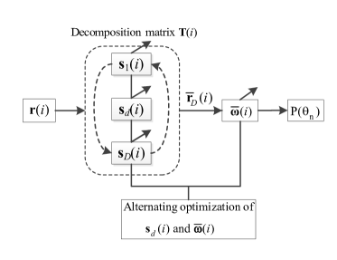
Figure 1: Block diagram of the ALRD scheme

III-A Proposed ALRD Scheme

The block diagram of the ALRD scheme is depicted in Fig. 1. The received vector $\mathbf{r}(i)=[r_{0}(i)\ldots r_{M-1}(i)]^{T}$ is processed by an $M\times D$ decomposition matrix ${\bf T}(i)$ which consists of a set of $I\times 1$ basis vectors $\mathbf{s}_{d}(i)$, where $d\in\{1,\ldots D\}$. The resulting data vector can be expressed by

$${\bf{\bar{r}}}_{D}(i)={\bf T}^{H}(i){\bf r}(i)=\sum_{d=1}^{D}{\bf{q}}_{d}{\bf{d}}^{H}_{d}\bm{\mathcal{R}}(i){\bf{s}}_{d}^{*}(i)$$ (4)

where ${\bf{q}}_{d}$ is a $D\times 1$ vector with a one in the $d$th position and zeros elsewhere. ${\bf{d}}_{d}$ is the $D\times 1$ selection vector to divide ${\bf{r}}(i)$ into $D$ segments, which are defined as:

$${\bf{d}}_{d}=[~{}\underbrace{0~{},\ldots~{},0~{}}_{\mu_{d}~{}zeros},~{}1~{},\underbrace{0~{},\ldots~{},0~{}}_{M-\mu_{d}-1~{}zeros}]^{T}$$ (5)

where $\mu_{d}$ is the selection pattern which is chosen as $\mu_{d}=(d-1)\lfloor\frac{M}{D}\rfloor$. The $M\times I$ matrix $\bm{\mathcal{R}}(i)$ corresponding to $\mathbf{r}(i)$ has a Hankel structure [29], which is described by

$$\bm{\mathcal{R}}(i)=\left(\begin{smallmatrix}r_{0}(i)&r_{1}(i)&\ldots&r_{I-1}(i)\\ \vdots&\vdots&\ldots&\vdots\\ r_{M-I}(i)&r_{M-I+1}(i)&\ldots&r_{M-1}(i)\\ r_{M-I+1}(i)&r_{M-I+2}(i)&\ldots&0\\ \vdots&\vdots&\ddots&\vdots\\ r_{M-2}(i)&r_{M-1}(i)&0&0\\ r_{M-1}(i)&0&0&0\\ \end{smallmatrix}\right)$$ (6)

The $I\times 1$ basis vectors $\mathbf{s}_{1}(i)\ldots\mathbf{s}_{D}(i)$ form the $M\times D$ decomposition matrix $\mathbf{T}(i)$. After dimensionality reduction, the $D\times 1$ data vector ${\bf{\bar{r}}}_{D}(i)$ is processed by an auxiliary parameter vector ${\bm{\bar{\omega}}}(i)$ to compute the output power spectrum. As seen from Fig. 1, the basis vectors $\mathbf{s}_{d}(i)$ and the auxiliary parameter vector ${\bm{\bar{\omega}}}(i)$ are alternately optimized according to some prescribed criterion, which is introduced in what follows.

III-B Proposed ALRD-RLS DOA Estimation Algorithm

The ALRD-RLS algorithm solves the optimization problem:

$$\begin{split}&\min_{\bm{\bar{\omega}}(i),\mathbf{s}_{d}(i)}\sum_{l=1}^{i}\alpha^{i-l}\big{|}\bm{\bar{\omega}}^{H}(i)\sum_{d=1}^{D}{\bf{q}}_{d}{\mathbf{d}}^{H}_{d}\bm{\mathcal{R}}(l){\bf{s}}_{d}^{*}(i)\big{|}^{2}\\ &\textrm{subject to}\quad\bm{\bar{\omega}}^{H}(i)\sum_{d=1}^{D}{\bf{q}}_{d}{\mathbf{d}}^{H}_{d}\bm{\mathcal{A}}_{n}{\bf{s}}_{d}^{*}(i)=1\end{split}$$ (7)

where $\alpha$ is a forgetting factor close to but smaller than $1$. $\bm{\mathcal{A}}_{n}$ is the $M\times I$ Hankel matrix of the scanning steering vector ${\bf{a}}(\theta_{n})=[a_{0}(\theta_{n})\ldots a_{M-1}(\theta_{n})]^{T}$ given by

$$\bm{\mathcal{A}}_{n}(i)=\left(\begin{smallmatrix}a_{0}(\theta_{n})&a_{1}(\theta_{n})&\ldots&a_{I-1}(\theta_{n})\\ \vdots&\vdots&\ldots&\vdots\\ a_{M-I}(\theta_{n})&a_{M-I+1}(\theta_{n})&\ldots&a_{M-1}(\theta_{n})\\ a_{M-I+1}(\theta_{n})&a_{M-I+2}(\theta_{n})&\ldots&0\\ \vdots&\vdots&\ddots&\vdots\\ a_{M-2}(\theta_{n})&a_{M-1}(\theta_{n})&0&0\\ a_{M-1}(\theta_{n})&0&0&0\\ \end{smallmatrix}\right).$$ (8)

The optimization problem in (7) can be solved by the method of Lagrange multipliers whose Lagrangian is described by

$$\begin{split}\mathcal{L}(i)&=\sum_{l=1}^{i}\alpha^{i-l}\big{|}\bm{\bar{\omega}}^{H}(i)\sum_{d=1}^{D}{\bf{q}}_{d}{\bf{d}}^{H}_{d}\bm{\mathcal{R}}(l){\bf{s}}_{d}^{*}(i)\big{|}^{2}\\ &\quad+2\mathfrak{R}\{\lambda[\bm{\bar{\omega}}^{H}(i)\sum_{d=1}^{D}{\bf{q}}_{d}{\mathbf{d}}^{H}_{d}\bm{\mathcal{A}}_{n}{\bf{s}}_{d}^{*}(i)-1]\}.\end{split}$$ (9)

where $\mathfrak{R}\{\cdot\}$ selects the real part of the argument. By taking the gradient of (9) with respect to ${\bf{s}}_{d}(i)$, we obtain

$$\begin{split}&\frac{\partial\mathcal{L}(i)}{\partial{\bf{s}}_{d}(i)}=\sum_{l=1}^{i}\alpha^{i-l}\bm{\mathcal{R}}^{H}(l){\bf{d}}_{d}{\bf{q}}^{H}_{d}\bm{\bar{\omega}}(i)\bm{\bar{\omega}}^{H}(i){\bf{q}}_{d}{\bf{d}}^{H}_{d}\bm{\mathcal{R}}(l){\bf{s}}_{d}^{*}(i)\\ &\quad+\sum_{l=1}^{i}\alpha^{i-l}\bm{\mathcal{R}}^{H}(i){\bf{d}}_{d}{\bf{q}}^{H}_{d}\bm{\bar{\omega}}(i)\bm{\bar{\omega}}^{H}(i)\sum_{j\neq d}^{D}{\bf{q}}_{j}{\bf{d}}^{H}_{j}\bm{\mathcal{R}}(l){\bf{s}}_{j}^{*}(i)\\ &\quad+\lambda^{*}\bm{\mathcal{A}}^{H}_{n}{\bf{d}}_{d}{\bf{q}}^{H}_{d}\bm{\bar{\omega}}(i).\end{split}$$ (10)

By equating (10) to zero and solving for ${\bf{s}}_{d}(i)$, we have

$${\bf{R}}_{s,d}(i){\bf{s}}_{d}(i)=-\sum_{j\neq d}^{D}{\bf{P}}_{s,j}(i)-\lambda\bm{\mathcal{A}}^{T}_{n}{\bf{d}}_{d}{\bf{q}}^{H}_{d}\bm{\bar{\omega}}^{*}(i)$$ (11)

where

$$\small{\bf{R}}_{s,d}(i)=\sum_{l=1}^{i}\alpha^{i-l}\bm{\mathcal{R}}^{T}(l){\bf{q}}_{d}{\bf{d}}^{H}_{d}\bm{\bar{\omega}}^{*}(i)\bm{\bar{\omega}}^{T}(i){\bf{q}}_{d}{\bf{d}}^{H}_{d}\bm{\mathcal{R}}^{*}(l)$$ (12)

$${\bf{P}}_{s,j}(i)=\sum_{l=1}^{i}\alpha^{i-l}\bm{\mathcal{R}}^{T}(l){\bf{d}}_{d}{\bf{q}}^{H}_{d}\bm{\bar{\omega}}^{*}(i)\bm{\bar{\omega}}^{T}(i){\bf{q}}_{j}{\bf{d}}^{H}_{j}\bm{\mathcal{R}}^{*}(l){\bf{s}}_{j}(i).$$ (13)

Then $I\times 1$ basis vector ${\bf{s}}_{d}(i)$ is described as:

$${\bf{s}}_{d}(i)=-{\bf{R}}_{s,d}^{-1}(i)\sum_{j\neq d}^{D}{\bf{P}}_{s,j}(i)-\lambda{\bf{R}}_{s,d}^{-1}(i)\bm{\mathcal{A}}^{T}_{n}{\bf{d}}_{d}{\bf{q}}^{H}_{d}\bm{\bar{\omega}}^{*}(i).$$ (14)

Substituting (14) into (7), we obtain the Lagrange multiplier:

$$\lambda=\frac{\sum\limits_{j\neq d}^{D}{\bf{q}}^{H}_{j}\bm{\bar{\omega}}(i){\bf{d}}^{H}_{d}\bm{\mathcal{A}}^{*}_{n}{\bf{s}}_{j}(i-1)-1-\mathbf{\bm{\prod}}(i){\bf{R}}_{s,d}^{-1}(i)\sum\limits_{j\neq d}^{D}{\bf{P}}_{s,j}(i)}{\bm{\prod}(i){\bf{R}}_{s,d}^{-1}(i)\bm{\prod}^{H}(i)}$$ (15)

where $\bm{\prod}(i)={\bf{q}}^{H}_{d}\bm{\bar{\omega}}(i){\bf{d}}^{H}_{d}\bm{\mathcal{A}}^{*}_{n}$. Based on (14) and (15), we obtain the $d$th basis vector ${\bf{s}}_{d}(i)$.

Next we consider the update of ${\bf{R}}_{s,d}^{-1}(i)$. By applying the matrix inversion lemma [20] to (12), we obtain

$$\begin{split}\small{\bf{g}}_{s,d}(i)=\frac{{\bf{R}}_{s,d}^{-1}(i-1)\bm{\mathcal{R}}^{T}(l){\bf{d}}_{d}}{\alpha\beta+{\bf{d}}^{H}_{d}\bm{\mathcal{R}}^{*}(l){\bf{R}}_{s,d}^{-1}(i-1)\bm{\mathcal{R}}^{T}(l){\bf{d}}_{d}}\end{split}$$ (16)

$${\bf{R}}_{s,d}^{-1}(i)=\alpha^{-1}{\bf{R}}_{s,d}^{-1}(i-1)-\alpha^{-1}{\bf{g}}_{s,d}(i){\bf{d}}^{H}_{d}\bm{\mathcal{R}}^{*}(l){\bf{R}}_{s,d}^{-1}(i-1)$$ (17)

where $\beta=({\bf{q}}^{H}_{d}\bm{\bar{\omega}}^{*}(i)\bm{\bar{\omega}}^{T}(i){\bf{q}}_{d})^{-1}$. As with ${\bf{P}}_{s,j}(i)$, we obtain it through iterations:

$$\begin{split}{\bf{P}}_{s,j}(i)=&\bm{\mathcal{R}}^{T}(l){\bf{d}}_{d}{\bf{q}}^{H}_{d}\bm{\bar{\omega}}^{*}(i)\bm{\bar{\omega}}^{T}(i){\bf{q}}_{j}{\bf{d}}^{H}_{j}\bm{\mathcal{R}}^{*}(l){\bf{s}}_{j}(i)\\ &+\alpha{\bf{P}}_{s,j}(i-1)\end{split}.$$ (18)

By employing (14)-(18), we can update ${\bf{s}}_{d}(i)$ for $d\in\{1,\ldots D\}$. Given the values of ${\bf{s}}_{d}(i)$, we can compute $\bm{\bar{\omega}}(i)$. Defining $\bar{\bf{a}}(i)=\sum_{d=1}^{D}{\bf{q}}_{d}{\mathbf{d}}^{H}_{d}\bm{\mathcal{A}}_{n}{\bf{s}}_{d}^{*}(i)$, (7) can be modified as

$$\begin{split}&\min_{\bm{\bar{\omega}}(i)}\quad\sum_{l=1}^{i}\alpha^{i-l}\big{|}\bm{\bar{\omega}}^{H}(i){\bf{\bar{r}}}_{D}(l)\big{|}^{2}\\ &\textrm{subject to}\quad\bm{\bar{\omega}}^{H}(i)\bar{\bf{a}}(i)=1\end{split}.$$ (19)

Solving for $\bm{\bar{\omega}}(i)$, we have

$${\bm{g}}_{D}(i)=\frac{{\bf{R}}_{D}^{-1}(i-1){\bf{\bar{r}}}_{D}(i)}{\alpha+{\bf{\bar{r}}}^{H}_{D}(i){\bf{R}}_{D}^{-1}(i-1){\bf{\bar{r}}}_{D}(i)}$$ (20)

$${\bf{R}}_{D}^{-1}(i)=\alpha^{-1}{\bf{R}}_{D}^{-1}(i-1)-\alpha^{-1}{\bm{g}}_{D}(i){\bf{\bar{r}}}^{H}_{D}(i){\bf{R}}_{D}^{-1}(i-1)$$ (21)

$$\bm{\bar{\omega}}(i)=\frac{{\bf{R}}_{D}^{-1}(i)\bar{\bf{a}}(i)}{\bar{\bf{a}}^{H}(i){\bf{R}}_{D}^{-1}(i)\bar{\bf{a}}(i)}$$ (22)

where ${\bf{R}}_{D}^{-1}(i)=\sum_{l=1}^{i}\alpha^{i-l}{\bf{\bar{r}}}_{D}(i){\bf{\bar{r}}}^{H}_{D}(i)$. Based on the previous derivations, we calculate the output power for each scanning angle $\theta_{n}$:

$$P(\theta_{n})=\sum_{l=1}^{i}\alpha^{i-l}\big{|}\bm{\bar{\omega}}^{H}(i){\bf{\bar{r}}}_{D}(i)\big{|}^{2}=\frac{1}{\bar{\bf{a}}^{H}(i){\bf{R}}_{D}^{-1}(i)\bar{\bf{a}}(i)}.$$ (23)

The ALRD-RLS algorithm is summarized in Table I.

TABLE I: The ALRD-RLS DOA estimation algorithm.

1   Set $N$ and $\alpha$

2   for each scanning angle $\theta_{n}$ do

3      Initialize $\mathbf{R}_{s,d}^{-1}(0)$, $\mathbf{P}_{s,j}(0)$, ${\bf{s}}_{d}(0)$, $\bm{\bar{\omega}}(0)$

4      for each snapshot $i$ ($i=1,\ldots,N$) do

5          for each basis $d$ ($d=1,\ldots,D$) do

6             Update ${\bf{s}}_{d}(i)$ based on (14)-(18).

7          Update $\bar{\bm{\omega}}(i)$ based on (20)-(22).

8      Calculate the output power $P(\theta_{n})=(\bar{\bf{a}}^{H}(N){\bf{R}}_{D}^{-1}(N)\bar{\bf{a}}(N))^{-1}$

9   Determine the estimated DOA $\hat{\bm{\theta}}=\textrm{arg}~{}\max_{\theta_{n}}~{}P(\theta_{n})$

III-C Proposed MALRD-RLS DOA Estimation Algorithm

By examining the structure of the ALRD scheme, we can reduce its computational cost by using a single basis vector in the decomposition matrix. From this observation, we come up with a modified version of the ALRD-RLS algorithm, i.e., the MALRD-RLS algorithm. Specifically, the columns of the decomposition matrix in the MALRD-RLS algorithm are formed by shifted versions of the same basis vector ${\bf{s}}(i)$, which results in ${\bf{\bar{r}}}_{D}(i)={\bf{Q}}\bm{\mathcal{R}}(i){\bf{s}}^{*}(i)$, where ${\bf{Q}}=\sum_{d=1}^{D}{\bf{q}}_{d}{\mathbf{d}}^{H}_{d}$. Therefore, the optimization problem solved by the MALRD-RLS algorithm is:

$$\begin{split}&\min_{\bm{\bar{\omega}}(i),\mathbf{s}(i)}\sum_{l=1}^{i}\alpha^{i-l}\big{|}\bm{\bar{\omega}}^{H}(i){\bf{Q}}\bm{\mathcal{R}}(l){\bf{s}}^{*}(i)\big{|}^{2}\\ &{\rm subject~{}~{}to}\quad\bm{\bar{\omega}}^{H}(i){\bf{Q}}\bm{\mathcal{A}}_{n}{\bf{s}}^{*}(i)=1\end{split}.$$ (24)

This problem can be solved by following the same procedure as in the ALRD-RLS algorithm. Firstly, we construct the Lagrangian function as

$$\begin{split}\mathcal{L}(i)&=\sum_{l=1}^{i}\alpha^{i-l}\big{|}\bm{\bar{\omega}}^{H}(i){\bf{Q}}\bm{\mathcal{R}}(l){\bf{s}}^{*}(i)\big{|}^{2}\\ &+2\mathfrak{R}\{\lambda[\bm{\bar{\omega}}^{H}(i){\bf{Q}}\bm{\mathcal{A}}_{n}{\bf{s}}^{*}(i)-1]\}.\end{split}$$ (25)

Secondly, we take the gradient of (25) with respect to ${\bf{s}}(i)$, set the result to zero and solve for ${\bf{s}}(i)$. The update equation of ${\bf{s}}(i)$ is given by

$${\bf{s}}(i)=\frac{{\bf{R}}_{s}^{-1}(i)\bm{\mathcal{A}}_{n}^{T}{\bf{Q}}^{T}\bm{\bar{\omega}}^{*}(i)}{\bm{\bar{\omega}}^{T}(i){\bf{Q}}\bm{\mathcal{A}}_{n}^{*}{\bf{R}}_{s}^{-1}(i)\bm{\mathcal{A}}_{n}^{T}{\bf{Q}}^{T}\bm{\bar{\omega}}^{*}(i)}$$ (26)

where ${\bf{R}}_{s}(i)=\sum_{l=1}^{i}\alpha^{i-l}\bm{\mathcal{R}}^{T}(l){\bf{Q}}^{T}\bm{\bar{\omega}}^{*}(i)\bm{\bar{\omega}}^{T}(i){\bf{Q}}\bm{\mathcal{R}}^{*}(l)$. The matrix ${\bf{R}}_{s}^{-1}(i)$ can be computed as:

$${\bf{g}}_{s}(i)=\frac{{\bf{R}}_{s}^{-1}(i-1)\bm{\mathcal{R}}^{T}(i){\bf{Q}}^{T}\bm{\bar{\omega}}^{*}(i)}{\alpha+\bm{\bar{\omega}}^{T}(i){\bf{Q}}\bm{\mathcal{R}}^{*}(i){\bf{R}}_{s}^{-1}(i-1)\bm{\mathcal{R}}^{T}(i){\bf{Q}}^{T}\bm{\bar{\omega}}^{*}(i)}$$ (27)

$$\small{\bf{R}}_{s}^{-1}(i)=\alpha^{-1}{\bf{R}}_{s}^{-1}(i-1)-\alpha^{-1}{\bf{g}}_{s}(i)\bm{\bar{\omega}}^{T}(i){\bf{Q}}\bm{\mathcal{R}}^{*}(i){\bf{R}}_{s}^{-1}(i-1).$$ (28)

Next, we discuss the update of $\bm{\bar{\omega}}(i)$. By redefining $\bar{\bf{a}}(i)={\bf{Q}}\bm{\mathcal{A}}_{n}{\bf{s}}^{*}(i)$, the cost function for the update of $\bm{\bar{\omega}}(i)$ is the same as that in (19). Hence $\bm{\bar{\omega}}(i)$ can also be constructed by (20)-(22) in the MALRD-RLS algorithm.

TABLE II: The MALRD-RLS DOA estimation algorithm.

1   Set $N$ and $\alpha$

2   for each scanning angle $\theta_{n}$ do

3      Initialize $\mathbf{R}_{s}^{-1}(0)$, ${\bf{s}}(0)$, $\bm{\bar{\omega}}(0)$

4      for each snapshot $i$ ($i=1,\ldots,N$) do

5          Update ${\bf{s}}(i)$ based on (26)-(28).

6          Redefine $\bar{\bf{a}}(i)={\bf{Q}}\bm{\mathcal{A}}_{n}{\bf{s}}^{*}(i)$ and update $\bar{\bm{\omega}}(i)$ based on (20)-(22).

7     Calculate the output power $P(\theta_{n})=(\bar{\bf{a}}^{H}(N){\bf{R}}_{D}^{-1}(N)\bar{\bf{a}}(N))^{-1}$

8   Determine the estimated DOA $\hat{\bm{\theta}}=\textrm{arg}~{}\max_{\theta_{n}}~{}P(\theta_{n})$

A brief summary of the MALRD-RLS algorithm is illustrated in Table II. After the update of ${\bf{s}}(i)$ and $\bar{\bm{\omega}}(i)$, we calculate the output power spectrum based on $P(\theta_{n})=\sum_{l=1}^{i}\alpha^{i-l}\big{|}\bm{\bar{\omega}}^{H}(i){\bf{\bar{r}}}_{D}(i)\big{|}^{2}=(\bar{\bf{a}}^{H}(i){\bf{R}}_{D}^{-1}(i)\bar{\bf{a}}(i))^{-1}$. The peaks of the power spectrum are the estimated DOAs.

III-D Computational Complexity

Here we detail the computational complexity of the proposed ALRD-RLS and MALRD-RLS algorithms and several existing DOA estimation algorithms. ESPRIT uses an EVD of $\mathbf{R}$, which has complexity of $O(M^{3})$. MUSIC employs both the EVD and grid search, resulting in a cost of $O(M^{3}+(180/\triangle)M^{2})$, with $\triangle$ being the search step. Matrix inversions and grid searches are essential for Capon, whose complexity is $O((180/\triangle)M^{3})$. For the AV and CG algorithms, the construction of the basis vectors leads to a complexity which is higher than that of the ESPRIT algorithm [12][13]. The JIO-RLS algorithm has a cost of $O((180/\triangle)N(M^{2}+D^{2}))$, with $D$ being the length of the reduced-rank received vector. ALRD-RLS avoids the EVD, the matrix inversion and the construction of the transformation matrix, and the update of $D$ basis vectors and an auxiliary parameter vector requires $O((180/\triangle)N(DI^{2}+D^{2}))$. MALRD-RLS only uses one basis vector and costs $O((180/\triangle)N(I^{2}+D^{2}))$. The computational complexity of the analyzed algorithms is depicted in Table LABEL:tab:complexity. Even in a large sensor array, $I$ and $D$ are small numbers, with $I\ll M$ and $D\ll M$, the cost of ALRD-RLS and MALRD-RLS can be less than those of the existing algorithms.

TABLE III: Comparison of Computational Complexity.

Algorithm	Complexity
ESPRIT [4]	$O(M^{3})$
MUSIC [3]	$O(M^{3}+(180/\triangle)M^{2})$
Capon [5]	$O((180/\triangle)M^{3})$
AV [12]	$O((180/\triangle)KM^{2})$
CG [13]	$O((180/\triangle)KM^{2})$
JIO-RLS [14]	$O((180/\triangle)N(M^{2}+D^{2})$
ALRD-RLS	$O((180/\triangle)N(DI^{2}+D^{2})$
MALRD-RLS	$O((180/\triangle)N(I^{2}+D^{2})$

IV Simulations

In this section, we evaluate the ALRD-RLS and MALRD-RLS algorithms through simulations. We compare ALRD-RLS and MALRD-RLS with MUSIC, ESPRIT, Capon, CG, AV and the JIO-RLS algorithms. A ULA with $M=60$ elements is adopted in the experiments. $K=15$ narrowband source signals impinge on the ULA from directions $\theta_{1},\ldots,\theta_{K}$, with $2$ of them being correlated and the others uncorrelated. The correlated source samples are generated from a first-order autoregressive process:

$$s_{1}\sim\mathcal{N}(0,\sigma^{2}_{s})~{}~{}\textrm{and}~{}~{}s_{2}(i)=\varrho s_{1}(i)+\sqrt{1-\varrho^{2}}e(i)$$ (29)

where $e\sim\mathcal{N}(0,\sigma^{2}_{s})$. $\varrho$ is the correlation coefficient fixed as $0.7$ in this work. We assume that a small number of snapshots are available for DOA estimation and fix $N=20$ in the simulations. The source signals with powers $\sigma^{2}_{s}=1$ are modulated by the binary phase shift keying (BPSK) scheme. The search step is chosen as $0.3^{o}$ for the algorithms based on grid search. We assume that the source DOAs are resolved if $|\hat{\theta}_{k}-\theta_{k}|<|\theta_{k}-\theta_{k-1}|/2$. In each experiment, 100 independent Monte Carlo runs are conducted to obtain the curves.

In the first example shown in Fig. 2, we plot the resolution probability versus the input signal-to-noise ratio (SNR) of the analyzed algorithms. We set the parameters for JIO-RLS to $D=5$ and $\lambda=0.998$. For MALRD-RLS and ALRD-RLS, we choose $I=12$, $D=5$, $\lambda=0.998$. Note that higher $I$ and $D$ yield higher probability of resolution, yet they lead to higher cost as well. We have examined the values of $I,D\in[3,15]$ and observed that $I=12$, $D=5$ provides a satisfactory performance with acceptable complexity. MALRD-RLS achieves the best performance in the large sensor arrays for different SNR values, followed by ALRD-RLS, MUSIC, JIO-RLS, Capon and ESPRIT. The AV and CG algorithms fail to resolve the DOAs for most of the SNR values when many sources are present. Note that MUSIC, ESPRIT, Capon, AV and CG require forward backward averaging (FBA) [30, 31] to ensure satisfactory performance for correlated signals.

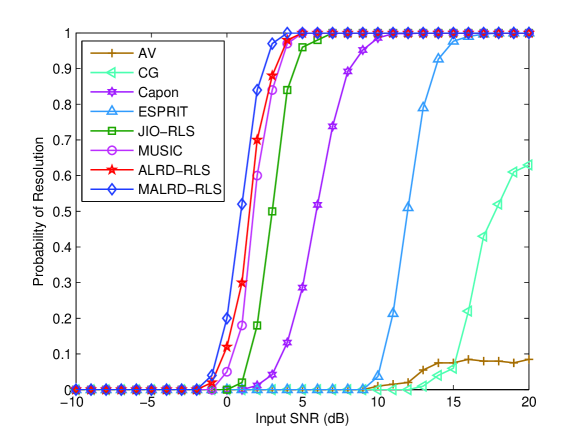
Figure 2: Probability of resolution versus input SNR.

We then evaluate the root mean square error (RMSE) performance of the analyzed algorithms, which is calculated as $RMSE=\sqrt{\frac{1}{NK}\sum_{n=1}^{N}\sum_{k=1}^{K}(\hat{\theta}_{k}-\theta_{k})^{2}}$. From Fig. 3, MALRD-RLS provides a superior RMSE performance with the lowest threshold SNR and the lowest RMSE level in high SNRs. The gap between the RMSE of MALRD-RLS and the Cramer-Rao bound (CRB) is due to the small number of available snapshots and the fact that the correlated sources degrade the performance.

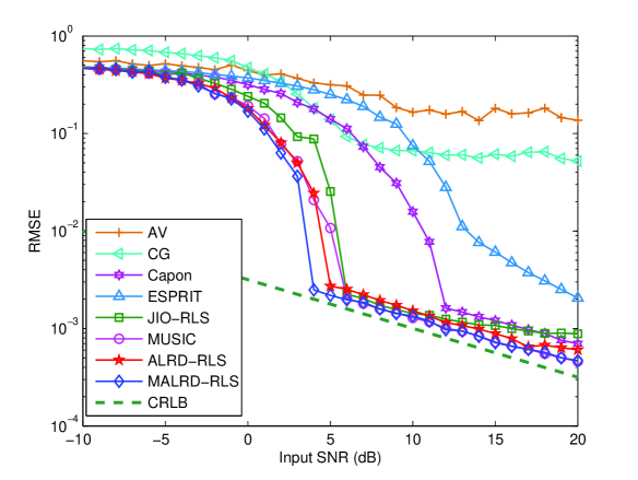
Figure 3: RMSE versus input SNR.

V Conclusion

In this paper, we have proposed the ALRD scheme and the ALRD-RLS and MALRD-RLS subspace DOA estimation algorithms based on alternating optimization. The proposed algorithms are suitable for large sensor arrays and have a lower computational cost than existing techniques. Simulation results show that MALRD-RLS and ALRD-RLS outperform previously reported algorithms.

References

• [1] H. Krim and M. Viberg, “Two decades of array signal processing research: the parametric approach,” IEEE Signal Processing Magazine, vol. 13, no. 4, pp. 67–94, July 1996.
• [2] H. L. V. Trees, Optimum Array Processing: Part IV of Detection, Estimation and Modulation Theory.   John Wiley $\&$ Sons, 2002.
• [3] R. O. Schmidt, “Multiple emitter location and signal parameter estimation,” IEEE Transactions on Antennas and Propagation, vol. 34, no. 3, pp. 276–280, March 1986.
• [4] R. Roy and T. Kailath, “ESPRIT-estimation of signal parameters via rotational invariance techniques,” IEEE Transactions on Acoustics, Speech and Signal Processing, vol. 37, no. 7, pp. 984–995, Jul. 1989.
• [5] J. Capon, “High-resolution frequency-wavenumber spectrum analysis,” Proceedings of the IEEE, vol. 57, no. 8, pp. 1408–1418, Aug. 1969.
• [6] K. C. Huarng and C. C. Yeh, “A unitary transformation method for angle-of-arrival estimation,” IEEE Transactions on Signal Processing, vol. 39, no. 4, pp. 975–977, April 1991.
• [7] F. G. Yan, M. Jin, and X. Qiao, “Low-complexity DOA estimation based on compressed MUSIC and its performance analysis,” IEEE Transactions on Signal Processing, vol. 61, no. 8, pp. 1915–1930, April 2013.
• [8] C. Qian, L. Huang, and H. C. So, “Improved unitary Root-MUSIC for DOA estimation based on pseudo-noise resampling,” IEEE Signal Processing Letters, vol. 21, no. 2, pp. 140–144, February 2014.
• [9] X. Mestre and M. A. Lagunas, “Modified subspace algorithms for doa estimation with large arrays,” IEEE Transactions on Signal Processing, vol. 56, no. 2, pp. 598–614, February 2008.
• [10] F. Gao and A. B. Gershman, “A generalized ESPRIT approach to direction-of-arrival estimation,” IEEE Signal Processing Letters, vol. 12, no. 3, pp. 254–257, March 2005.
• [11] N. Tayem and H. M. Kwon, “Conjugate ESPRIT (C-SPRIT),” IEEE Transactions on Antennas and Propagation, vol. 52, no. 10, pp. 2618–2624, Oct. 2004.
• [12] R. Grover, D. A. Pados, and M. J. Medley, “Subspace direction finding with an auxiliary-vector basis,” IEEE Transactions on Signal Processing, vol. 55, no. 2, pp. 758–763, January 2007.
• [13] H. Semira, H. Belkacemi, and S. Marcos, “High resolution source locallization algorithm based on the conjugate gradients,” EURASIP Journal on Advances in Signal Processing, vol. 2007, pp. 1–9, March 2007.
• [14] L. Wang, R. C. de Lamare, and M. Haardt, “Direction finding algorithms based on joint iterative subspace optimization,” IEEE Trans. Aerosp. Electron. Syst., vol. 50, no. 4, pp. 2541–2553, Oct. 2014.
• [15] H. B. Lee and M. Wengrovitz, “Resolution threshold of beamspace MUSIC for two closely spaced emitters,” IEEE Trans. Acoustics, Speech and Signal Process., vol. 38, no. 9, pp. 1545–1559, Sep. 1990.
• [16] M. D. Zoltowski, G. M. Kautz, and S. D. Silverstein, “Beamspace Root-MUSIC,” IEEE Transactions on Signal Processing, vol. 41, no. 1, pp. 344–, January 1993.
• [17] G. H. Xu, S. D. Silverstein, R. H. Roy, and T. Kailath, “Beamspace ESPRIT,” IEEE Transactions on Signal Processing, vol. 42, no. 2, pp. 349–356, Feb. 1994.
• [18] J. Steinwandt, R. C. de Lamare, and M. Haardt, “Beamspace direction finding based on the conjugate gradient and the auxiliary vector filtering algorithms,” Elsevier Signal Processing, vol. 93, pp. 641–651, 2013.
• [19] A. Hassanien, S. A. Elkader, A. B. Gershman, and K. M. Wong, “Convex optimization based beam-space preprocessing with improved robustness against out-of-sector sources,” IEEE Transactions on Signal Processing, vol. 54, no. 5, pp. 1587–1595, May 2006.
• [20] S. Haykin, Adaptive Filter Theory.   Englewood Cliffs, NJ: Prentice Hall, 2002.
• [21] R. C. de Lamare and R. C. de Lamare, “Adaptive reduced-rank mmse filtering with interpolated fir filters and adaptive interpolators,” IEEE Signal Processing Letters, vol. 12, no. 3, March 2005.
• [22] R. C. de Lamare and R. Sampaio-Neto, “Reduced–rank adaptive filtering based on joint iterative optimization of adaptive filters,” IEEE Signal Process. Lett., vol. 14, no. 12, pp. 980–983, December 2007.
• [23] ——, “Adaptive reduced-rank equalization algorithms based on alternating optimization design techniques for MIMO systems,” IEEE Transactions on Vehicular Technology, vol. 60, no. 6, pp. 2482–2494, July 2011.
• [24] ——, “Reduced-rank space–time adaptive interference suppression with joint iterative least squares algorithms for spread-spectrum systems,” IEEE Transactions Vehicular Technology, vol. 59, no. 3, pp. 1217–1228, March 2010.
• [25] ——, “Adaptive reduced-rank processing based on joint and iterative interpolation, decimation and filtering,” IEEE Trans. Signal Processing, vol. 57, no. 7, pp. 2503–2514, July 2009.
• [26] R. Fa, R. C. de Lamare, and L. Wang, “Reduced-rank stap schemes for airborne radar based on switched joint interpolation, decimation and filtering algorithm,” IEEE Transactions on Signal Processing, vol. 58, no. 8, pp. 4182–4194, August 2010.
• [27] S. Li, R. C. de Lamare, and R. Fa, “Reduced-rank linear interference suppression for ds-uwb systems based on switched approximations of adaptive basis functions,” IEEE Transactions on Vehicular Technology, vol. 60, no. 2, pp. 485–497, Feb 2011.
• [28] R. C. de Lamare, R. Sampaio-Neto, and M. Haardt, “Blind adaptive constrained constant-modulus reduced-rank interference suppression algorithms based on interpolation and switched decimation,” IEEE Transactions on Signal Processing, vol. 59, no. 2, pp. 681–695, Feb 2011.
• [29] G. H. Golub and C. F. van Loan, Matrix Computations.   New York: Wiley, 2002.
• [30] S. U. Pillai and B. H. Kwon, “Forward/backward spatial smoothing techniques for coherent signal identification,” IEEE Transactions on Acoustics, Speech and Signal Processing, vol. 37, no. 1, pp. 8–15, January 1989.
• [31] D. A. Linebarger, R. D. DeGroat, and E. M. Dowling, “Efficient direction-finding methods employing forward/backward averaging,” IEEE Transactions on Signal Processing, vol. 42, no. 8, pp. 2136–2145, August 1994.