Unsupervised Nonlinear Spectral Unmixing based on a Multilinear Mixing Model

Abstract

In the community of remote sensing, nonlinear mixing models have recently received particular attention in hyperspectral image processing. In this paper, we present a novel nonlinear spectral unmixing method following the recent multilinear mixing model of [1], which includes an infinite number of terms related to interactions between different endmembers. The proposed unmixing method is unsupervised in the sense that the endmembers are estimated jointly with the abundances and other parameters of interest, i.e., the transition probability of undergoing further interactions. Non-negativity and sum-to-one constraints are imposed on abundances while only non-negativity is considered for endmembers. The resulting unmixing problem is formulated as a constrained nonlinear optimization problem, which is solved by a block coordinate descent strategy, consisting of updating the endmembers, abundances and transition probability iteratively. The proposed method is evaluated and compared with linear unmixing methods for synthetic and real hyperspectral datasets acquired by the AVIRIS sensor. The advantage of using non-linear unmixing as opposed to linear unmixing is clearly shown in these examples.

I Introduction

Spectral unmixing (SU) aims at decomposing a set of $n$ multivariate measurements (or pixel vectors) ${\mathbf{X}}=\left[{\mathbf{x}}^{1},\ldots,{\mathbf{x}}^{n}\right]$ into a collection of $m$ elementary signatures ${\mathbf{E}}=\left[{\mathbf{e}}_{1},\cdots,{\mathbf{e}}_{m}\right]$, usually referred to as endmembers, and estimating the relative proportions ${\mathbf{A}}=\left[{\mathbf{a}}^{1},\ldots,{\mathbf{a}}^{n}\right]$ of these signatures, called abundances. SU has been advocated as a relevant multivariate analysis technique in various applicative areas, including remote sensing [2], planetology [3], microscopy [4], spectroscopy [5] and gene expression analysis [6]. In particular, a great interest has been demonstrated when analyzing multi-band (e.g., hyperspectral) images, for instance for pixel classification [7], material quantification [8] and subpixel detection [9].

I-A Linear Mixture Model

The linear mixture model (LMM) assumes that each image pixel is a linear combination of all the endmembers present in this pixel. The LMM model has been widely used in the remote sensing community and can be expressed as (see, e.g., [10])

$${\mathbf{x}}^{i}={\mathbf{E}}{\mathbf{a}}^{i}+{\mathbf{n}}^{i}$$ (1)

where

• ${\mathbf{x}}^{i}$ is a $d\times 1$ vector representing the measured reflectance for the $i$th pixel,

• ${\mathbf{E}}\in\mathbb{R}^{d\times m}$ is a non-negative matrix whose columns ${\mathbf{e}}_{1},\cdots,{\mathbf{e}}_{m}$ correspond to $m$ endmember signatures and span the space where the data ${\mathbf{x}}^{1},\ldots,{\mathbf{x}}^{n}$ reside,

• ${\mathbf{a}}^{i}$ is an $m\times 1$ non-negative vector, which includes the fractional abundances (coefficients) for the $i$th pixel (that sum to $1$),

• ${\mathbf{n}}^{i}\in\mathbb{R}^{d}$ is the additive Gaussian noise.

By arranging all pixels of the observed scenario lexicographically, the LMM model can be written as

$$\bf X=EA+N$$ (2)

where ${\mathbf{X}}\in\mathbb{R}^{d\times n}$, ${\mathbf{A}}\in\mathbb{R}^{m\times n}$ and ${\mathbf{N}}\in\mathbb{R}^{d\times n}$ are the reflectance, abundance and noise matrices, $n$ is the number of observations, and $d$ is the number of spectral bands.

The spectral unmixing problem based on the LMM is generally formulated as the following constrained least squares problem.

$$\begin{aligned} &\min_{{\mathbf{a}}^{i}}\|{{{\mathbf{x}}^{i}-{\mathbf{E}}{\mathbf{a}}^{i}}}\|_{2}^{2}\\ &\text{subject to (s.t.)}\quad{\mathbf{a}}^{i}\geq 0\quad\textrm{and}\quad{\bf 1}^{T}_{m}{{\mathbf{a}}^{i}}=1\end{aligned}$$ (3)

where ${\bf 1}_{m}$ is an $m\times 1$ vector with all ones. Using all observed data and matrix notations, the optimization problem can be written as

$$\begin{aligned} &\min_{\bf A}\|{{\bf X-EA}}\|_{F}^{2}\\ &\text{s.t.}\quad\textbf{A}\geq 0\quad\textrm{and}\quad{\bf 1}^{T}_{m}{\bf A}={\bf 1}_{n}^{T}\end{aligned}$$ (4)

where $\textbf{A}\geq 0$ has to be understood in the element-wise sense, meaning that all the coefficients are non-negative. Note that $\|\cdot\|_{F}$ is the Frobenius norm, which is defined as

$$\|{\mathbf{X}}\|_{F}=\sqrt{\text{trace}({\mathbf{X}}^{H}{\mathbf{X}})}$$

where ${\mathbf{X}}^{H}$ denotes the conjugate transpose of ${\mathbf{X}}$ and trace(${\mathbf{M}}$) is the trace of the matrix ${\mathbf{M}}$ [11].

I-B Nonlinear Mixture Model

Due to its simple and intuitive physical interpretation as well as tractable estimation process, the LMM has been widely used for unmixing, and has shown interesting results in various applications. However, there exist many scenarios in which the LMM is not appropriate and can be advantageously replaced by a nonlinear mixing model [12, 1]. One notable example is the case of scenes with large geometrical structures such as buildings or trees, where shadowing and mutual illumination involve multiple light scattering effects. Another example is the case of mineral mixtures (also referred to as intimate mixtures), where an incoming light ray can interact many times with the different mineral grains, and the single interactions assumed in the LMM can even become relatively rare. Furthermore, the LMM only considers reflection and disregards optical transmission, which can become quite important in vegetation and mineral mixtures. To solve these problems, nonlinear mixture models have been proposed as interesting alternatives to overcome the inherent limitations of the LMM. These models include the Hapke model [13], the generalized bilinear model (GBM) [14, 15], the linear-quadratic model [16], the post-nonlinear mixing model (PNMM) [17] and the multi-linear mixing (MLM) model [1].

In this work, we focus on the recently proposed MLM model [1] as follows

$$\begin{split}{\mathbf{x}}^{i}&=(1-P^{i}){\mathbf{y}}^{i}+(1-P^{i})P^{i}({\mathbf{y}}^{i}\odot{\mathbf{y}}^{i})\\ &+(1-P^{i})(P^{i})^{2}({\mathbf{y}}^{i}\odot{\mathbf{y}}^{i}\odot{\mathbf{y}}^{i})\cdots\end{split}$$ (5)

where ${\mathbf{x}}^{i}$ represents the observed reflectance, ${\mathbf{y}}^{i}={\mathbf{E}}{\mathbf{a}}^{i}$ is the linear term used in the traditional LMM model, $\odot$ represents the Hadamard entry-wise product and $P^{i}$ represents the probability of undergoing further interactions after each interaction with a material. Thus, $1-P_{i}$ corresponds to the probability of escaping the scene and reaching the observer. The MLM model is the first nonlinear model that includes all orders of interactions by introducing only a single parameter $P^{i}$, which describes the probability of further interactions. Furthermore, the summation in (5) can be conveniently simplified as the following fixed-point equation

$${\mathbf{x}}^{i}=(1-P^{i}){\mathbf{y}}^{i}+P^{i}{\mathbf{y}}^{i}\odot{\mathbf{x}}^{i}.$$ (6)

Note that $P^{i}$ is different from pixel to pixel. For more details concerning the derivation of the MLM, we refer the reader to [1]. To achieve nonlinear unmixing, the authors of [1] considered the following optimization problem

$$\begin{split}&\mathrm{arg}\min_{\{{\mathbf{a}}^{i},P^{i}\}}\|{{\mathbf{x}}^{i}-\frac{(1-P^{i}){\mathbf{y}}^{i}}{1-P^{i}{\mathbf{y}}^{i}}}\|_{2}^{2}\\ &\textrm{ s.t. }\quad{\mathbf{y}}^{i}={\mathbf{E}}{\mathbf{a}}^{i}.\end{split}$$ (7)

The endmember matrix ${\mathbf{E}}$ was suggested to be estimated using VCA [18], which is one of the state-of-the-art endmember extraction methods, and to be fixed in the unmixing, leading to a supervised unmixing method. However, the VCA algorithm is based on the LMM model, which is different from the MLM. Furthermore, the optimization w.r.t. ${\mathbf{a}}^{i}$ and $P^{i}$ is highly nonlinear and nonconvex, preventing a unique solution from being obtained.

To overcome the difficulties mentioned above, this work considers three main modifications with respect to the method in [1]. First, the objective function is slightly changed from (7), in order to avoid its highly nonlinearity and nonconvexity w.r.t. the parameters to be estimated. This modification significantly decreases the complexity of the optimization problem (7), which will be illustrated later. Second, instead of fixing the endmember matrix using VCA, the output of VCA is used as an initialization of an algorithm, which estimates the endmember matrix jointly with the abundances and the transition probability, leading to an unsupervised nonlinear mixing strategy. Finally, the parameter $P_{i}$ is constrained to belong to the interval [0,1], which is in agreement with its probability interpretation.

II Nonlinear Spectral Unmixing: A BCD scheme

The nonlinear unmixing problem investigated in this work can be formulated as the following optimization problem

$$\mathrm{arg}\min_{\{{\mathbf{a}}^{i},P^{i}\}_{i=1}^{m},{\mathbf{E}}}L({\mathbf{E}},{\mathbf{A}},{\mathbf{P}})$$ (8)

$$\begin{split}\textrm{ with }\quad L({\mathbf{E}},{\mathbf{A}},{\mathbf{P}})&=\sum_{i=1}^{n}\|{\mathbf{x}}^{i}-(1-P^{i}){\mathbf{y}}^{i}-P^{i}{\mathbf{y}}^{i}\odot{\mathbf{x}}^{i}\|_{2}^{2}\\ {\mathbf{y}}^{i}&={\mathbf{E}}{\mathbf{a}}^{i}\\ {\mathbf{a}}^{i}&\geq 0\quad\textrm{and}\quad{\bf 1}^{T}_{m}{{\mathbf{a}}^{i}}=1\\ 0&\leq{\mathbf{E}}\leq 1\\ 0&\leq P^{i}\leq 1.\end{split}$$

To solve the problem (8), we propose to update ${\mathbf{a}}^{i}$, ${\mathbf{E}}$ and ${\mathbf{P}}^{i}$ alternately, using a block coordinate descent (BCD) strategy. Even though (8) is a nonconvex problem w.r.t. ${\mathbf{a}}^{i}$, ${\mathbf{E}}$ and ${\mathbf{P}}^{i}$ jointly, it is interesting to note that each sub-problem turns out to be a convex problem which has a unique solution. The BCD algorithm is known to converge to a stationary point of the objective function to be optimized provided that this objective function has a unique minimum point w.r.t. each variable [19, Prop. 2.7.1], which is the case for the criterion in (8). Thus, the BCD algorithm introduced in this paper converges to a stationary point of (8). Note that the nonlinear unmixing problem (8) includes a linear unmixing (abundance estimation) step, an endmember extraction step and a transition probability estimation step. To ease the notation, we omit the upper indices $i$ for ${\mathbf{a}}$ and ${\mathbf{P}}$ hereafter as they can be updated pixel by pixel in parallel. It is worthy of note that one popular strategy to overcome the nonconvexity could be simulation based methods such as Markov Chain Monte Carlo (see [20] for a recent review). Such an approach would be computationally intensive, but could potentially yield improvement in performance and better estimation of the uncertainty inherent in the problem. However, the major drawback of being computationally expensive for simulation based methods prevents their effective use in this application.

II-A Optimization w.r.t. ${\mathbf{a}}$

The optimization w.r.t. ${\mathbf{a}}$ is now expressed as

$$\mathrm{arg}\min_{{\mathbf{a}}}\|{\mathbf{x}}-(1-P){\mathbf{E}}{\mathbf{a}}-P\left({\mathbf{E}}{\mathbf{a}}\right)\odot{\mathbf{x}}\|_{2}^{2}$$ (9)

$$\textrm{ s.t. }{\mathbf{a}}\geq 0\quad\textrm{and}\quad{\bf 1}^{T}_{m}{{\mathbf{a}}}=1.$$

Straightforward computations lead to the following equivalent optimization problem

$$\mathrm{arg}\min_{{\mathbf{a}}}\|{\mathbf{x}}-\tilde{{\mathbf{E}}}{\mathbf{a}}\|_{2}^{2}\textrm{\quad s.t. \quad}{\mathbf{a}}\geq 0\quad\textrm{and}\quad{\bf 1}^{T}_{m}{{\mathbf{a}}}=1$$ (10)

where $\tilde{{\mathbf{E}}}={\mathbf{E}}\odot\left[(1-P){\bf 1}_{d\times m}+P{\mathbf{x}}{\bf 1}^{T}_{m}\right]$. Thus, the optimization w.r.t. ${\mathbf{a}}$ becomes a standard fully constrained least squares (FCLS) problem with a modified endmember matrix $\tilde{{\mathbf{E}}}$. To solve this classical convex problem, there exist plenty of methods, e.g., active-set [21], ADMM [22] (sometimes referred to as SUNSAL [23]), projection-based methods [24], etc. Instead of solving (10) exactly, we use the gradient projection method [25, 26] to decrease the objective function defined in (10). More specifically, by denoting $g({\mathbf{a}})=\|{\mathbf{x}}-\tilde{{\mathbf{E}}}{\mathbf{a}}\|_{2}^{2}$, (10) can be rewritten as

$$\mathrm{arg}\min_{{\mathbf{a}}}g({\mathbf{a}})\textrm{\quad s.t. \quad}{\mathbf{a}}\in{\mathcal{A}}$$ (11)

where ${\mathcal{A}}=\left\{{\mathbf{a}}\in\mathbb{R}^{m}|{\mathbf{a}}\geq 0\textrm{ and }{\bf 1}^{T}_{m}{{\mathbf{a}}}=1\right\}$. Thus, the gradient of the objective $g({\mathbf{a}})$ w.r.t. ${\mathbf{a}}$ can be calculated as

$$\nabla_{{\mathbf{a}}}g({\mathbf{a}})=\tilde{{\mathbf{E}}}^{T}(\tilde{{\mathbf{E}}}{\mathbf{a}}-{\mathbf{x}}).$$

Note that the gradient projection method is different from the conventional gradient descent method in that each update after a move along the gradient direction $\nabla_{{\mathbf{a}}}g({\mathbf{a}})$ is projected onto the convex set ${\mathcal{A}}$ to force all the updates to belong to the set of feasible solutions, i.e.,

$${{\mathbf{a}}}=\Pi_{{\mathcal{A}}}\left({\mathbf{a}}-\gamma_{{\mathbf{a}}}\nabla_{{\mathbf{a}}}g({\mathbf{a}})\right),\quad\varepsilon\leq\gamma_{{\mathbf{a}}}\leq 2/L_{{\mathbf{a}}}-\varepsilon$$ (12)

where $\Pi_{{\mathcal{A}}}$ denotes the projection operator onto ${\mathcal{A}}$, $\varepsilon\in]0,\textrm{min}\{1,1/L_{{\mathbf{a}}}\}[$ and $L_{{\mathbf{a}}}=\|\tilde{{\mathbf{E}}}^{T}\tilde{{\mathbf{E}}}\|_{F}$ is the Lipschitz constant of $\nabla_{{\mathbf{a}}}g({\mathbf{a}})$. The projection onto the (canonical) simplex ${\mathcal{A}}$ can be achieved with a finite algorithm, such as Michelot [27], Duchi et al. [28], Condat [29], etc.

The motivation to use this gradient projection algorithm is two-fold. First, the convergence of a gradient projection within a BCD scheme is guaranteed (see more details in [30, 31, 32]). Second, the update (12) is less computationally intensive than solving the optimization problem (10) exactly which requires iterative updates. In this work, the stepsize $\gamma_{{\mathbf{a}}}$ is fixed to $1/L_{{\mathbf{a}}}$ to ensure a sufficient decrease of the objective value per iteration. The updating scheme for ${\mathbf{a}}$ is summarized in Algorithm 1. The computational complexity to calculate the abundances for all pixels is of the order ${\mathcal{O}}(\max\{d,m\}nm)$.

Input: ${\mathbf{a}}$, ${\mathbf{E}}$, ${\mathbf{x}}$, $P$

/* Calculate the modified endmembers (pixel-wised) */

1 $\tilde{{\mathbf{E}}}\leftarrow{\mathbf{E}}\odot\left((1-P){\bf 1}_{d\times m}+P{\mathbf{x}}{\bf 1}^{T}_{m}\right)$;

/* Calculate the Lipschitz constant */

2 $L_{{\mathbf{a}}}\leftarrow\|\tilde{{\mathbf{E}}}^{T}\tilde{{\mathbf{E}}}\|_{F}$;

/* Gradient projection update */

3 $\hat{{\mathbf{a}}}\leftarrow\Pi_{{\mathcal{A}}}\left({\mathbf{a}}-\nabla_{{\mathbf{a}}}g({\mathbf{a}})/L_{{\mathbf{a}}}\right)$;

Output: $\hat{{\mathbf{a}}}$

Algorithm 1 Minimization w.r.t. ${\mathbf{a}}$

II-B Optimization w.r.t. $P$

The optimization w.r.t. $P$ can be formulated as

$$\mathrm{arg}\min_{P}\|{\mathbf{x}}-(1-P){\mathbf{y}}-P{\mathbf{y}}\odot{\mathbf{x}}\|_{2}^{2}$$ (13)

$$\textrm{ s.t. }0\leq P\leq 1.$$

Obviously, problem (13) is convex and admits the following closed-form solution

$$\hat{P}=\Pi_{{[0,1]}}\left(\frac{({\mathbf{y}}-{\mathbf{y}}\odot{\mathbf{x}})^{T}({\mathbf{y}}-{\mathbf{x}})}{\|{\mathbf{y}}-{\mathbf{y}}\odot{\mathbf{x}}\|_{2}^{2}}\right)$$ (14)

where $[0,1]$ corresponds to the box constraints and $\bf y=Ea$. Furthermore, it is interesting to note that if $0\leq{\mathbf{y}}\leq 1$, the unconstrained solution $\frac{({\mathbf{y}}-{\mathbf{y}}\odot{\mathbf{x}})^{T}({\mathbf{y}}-{\mathbf{x}})}{\|{\mathbf{y}}-{\mathbf{y}}\odot{\mathbf{x}}\|_{2}^{2}}$ satisfies the box constraint automatically. Thus, the updates of $P$ can be simplified as

$$\hat{P}=\frac{({\mathbf{y}}-{\mathbf{y}}\odot{\mathbf{x}})^{T}({\mathbf{y}}-{\mathbf{x}})}{\|{\mathbf{y}}-{\mathbf{y}}\odot{\mathbf{x}}\|_{2}^{2}}.$$ (15)

The computational complexity to calculate the probability $P$ for all pixels is of the order ${\mathcal{O}}(nd)$.

II-C Optimization w.r.t. ${\mathbf{E}}$

The optimization of the objective function in (8) w.r.t. ${\mathbf{E}}$ can be formulated as

$$\mathrm{arg}\min_{{\mathbf{E}}}\|{\mathbf{x}}-(1-P){\mathbf{E}}{\mathbf{a}}-P\left({\mathbf{E}}{\mathbf{a}}\right)\odot{\mathbf{x}}\|_{2}^{2}$$ (16)

$$\textrm{ s.t. }0\leq{\mathbf{E}}\leq 1.$$

The above problem can be equivalently rewritten as

$$\mathrm{arg}\min_{{\mathbf{E}}}\|{\mathbf{x}}-\left({\mathbf{E}}\odot\tilde{{\mathbf{A}}}\right){\bf 1}_{m}\|_{2}^{2}\textrm{\quad s.t. \quad}0\leq{\mathbf{E}}\leq 1$$ (17)

where $\tilde{{\mathbf{A}}}=\left((1-P){\bf 1}_{d}+P{\mathbf{x}}\right){\mathbf{a}}^{T}$. Considering all the observed pixels leads to

$$\mathrm{arg}\min_{{\mathbf{E}}}f({\mathbf{E}})\textrm{\quad s.t. \quad}0\leq{\mathbf{E}}\leq 1$$ (18)

where $f({\mathbf{E}})=\sum_{i=1}^{n}\|{\mathbf{x}}^{i}-\left({\mathbf{E}}\odot\tilde{{\mathbf{A}}}^{i}\right){\bf 1}_{m}\|_{2}^{2}$ and $\tilde{{\mathbf{A}}}^{i}=\left((1-P^{i}){\bf 1}_{d}+P^{i}{\mathbf{x}}^{i}\right){({\mathbf{a}}^{i})^{T}}$. The gradient of the objective $f({\mathbf{E}})$ can therefore be calculated as follows

$$\begin{split}\nabla_{{\mathbf{E}}}f({\mathbf{E}})&=\sum_{i=1}^{n}\left[\left({\mathbf{E}}\odot\tilde{{\mathbf{A}}}^{i}\right){\bm{1}}_{m}-{\mathbf{x}}^{i}\right]{\bm{1}}_{m}^{T}\odot\tilde{{\mathbf{A}}}^{i}\\ &=\sum_{i=1}^{n}\left[\begin{array}[]{cc}({\mathbf{e}}_{1}\odot\tilde{{\mathbf{a}}}^{i}_{1}\odot\tilde{{\mathbf{a}}}^{i}_{1}+\cdots+{\mathbf{e}}_{m}\odot\tilde{{\mathbf{a}}}^{i}_{m}\odot\tilde{{\mathbf{a}}}^{i}_{1})^{T}\\ ({\mathbf{e}}_{1}\odot\tilde{{\mathbf{a}}}^{i}_{1}\odot\tilde{{\mathbf{a}}}^{i}_{2}+\cdots+{\mathbf{e}}_{m}\odot\tilde{{\mathbf{a}}}^{i}_{m}\odot\tilde{{\mathbf{a}}}^{i}_{2})^{T}\\ \vdots\\ ({\mathbf{e}}_{1}\odot\tilde{{\mathbf{a}}}^{i}_{1}\odot\tilde{{\mathbf{a}}}^{i}_{m}+\cdots+{\mathbf{e}}_{m}\odot\tilde{{\mathbf{a}}}^{i}_{m}\odot\tilde{{\mathbf{a}}}^{i}_{m})^{T}\end{array}\right]^{T}\\ &-\sum_{i=1}^{n}\left[\begin{array}[]{cc}({\mathbf{x}}^{i}\odot\tilde{{\mathbf{a}}}^{i}_{1})^{T}\\ ({\mathbf{x}}^{i}\odot\tilde{{\mathbf{a}}}^{i}_{2})^{T}\\ \vdots\\ ({\mathbf{x}}^{i}\odot\tilde{{\mathbf{a}}}^{i}_{m})^{T}\end{array}\right]^{T}\end{split}$$ (19)

where ${\mathbf{E}}=[{\mathbf{e}}_{1},\cdots,{\mathbf{e}}_{m}]$ and $\tilde{{\mathbf{A}}}^{i}=[\tilde{{\mathbf{a}}}_{1}^{i},\cdots,\tilde{{\mathbf{a}}}_{m}^{i}]$. The second order derivative (Hessian matrix) of $f({\mathbf{E}})$ w.r.t. ${\mathbf{E}}$ is a tensor and not easy to be expressed explicitly. Thanks to the Hadamard product, the second order derivative can be computed row by row. More specifically, for the $i$th row of ${\mathbf{E}}$, denoted as $\bm{\epsilon}^{j}(\in\mathbb{R}^{1\times m})$, we have

$$\nabla^{2}_{\bm{\epsilon}^{j}}f(\bm{\epsilon}^{j})=\sum\limits_{i=1}^{n}\left[\begin{array}[]{ccc}\tilde{a}_{1,j}^{i}\tilde{a}_{1,j}^{i}&\cdots&\tilde{a}_{1,j}^{i}\tilde{a}_{m,j}^{i}\\ \tilde{a}_{2,j}^{i}\tilde{a}_{1,j}^{i}&\cdots&\tilde{a}_{2,j}^{i}\tilde{a}_{m,j}^{i}\\ \vdots\\ \tilde{a}_{m,j}^{i}\tilde{a}_{1,j}^{i}&\cdots&\tilde{a}_{m,j}^{i}\tilde{a}_{m,j}^{i}\end{array}\right]$$ (20)

where $\tilde{a}_{l,j}^{i}$ represents the element of the matrix $\tilde{A}^{i}$ located in the $l$th row and in the $j$th column and $j=1,\cdots,d$. Thus, the Hessian matrix (or Lipschitz constant) of $\nabla_{{\mathbf{E}}}f({\mathbf{E}})$ can be computed row by row.

Similar to the update of ${\mathbf{A}}$, the gradient projection method can be implemented as follows

$$\bm{\epsilon}^{j}=\Pi_{{[0,1]}^{1\times m}}\left\{\bm{\epsilon}^{j}-\gamma_{\bm{\epsilon}^{j}}\nabla_{\bm{\epsilon}^{j}}f(\bm{\epsilon}^{j})\right\},\quad\varepsilon\leq\gamma_{\bm{\epsilon}^{j}}\leq 2/{L_{\bm{\epsilon}^{j}}}-\varepsilon$$ (21)

where $\varepsilon\in]0,\textrm{min}\{1,1/L_{\bm{\epsilon}^{j}}\}[$ and $L_{\bm{\epsilon}^{j}}=\|\nabla^{2}_{\bm{\epsilon}^{j}}f(\bm{\epsilon}^{j})\|_{F}$. The computational complexity to calculate the endmember matrix ${\mathbf{E}}$ is of the order ${\mathcal{O}}(\max\{md,m^{2}\}n)$. In this work, the stepsize $\gamma_{\bm{\epsilon}^{j}}$ is fixed to $1/L_{\bm{\epsilon}^{j}}$ to ensure a sufficient decrease of the objective value per iteration. The update of ${\mathbf{E}}$ is summarized in Algorithm 2.

Input: ${\mathbf{E}}$, ${\mathbf{a}}^{1:n}$, ${\mathbf{x}}^{1:n}$, $P^{1:n}$

/* Compute the temporary variable ${\tilde{{\mathbf{A}}}^{i}}$ */

1 ${\tilde{{\mathbf{A}}}^{i}}\leftarrow\left((1-P^{i}){\bf 1}_{d}+P^{i}{\mathbf{x}}^{i}\right){{\mathbf{a}}^{iT}}$ for $i=1,\cdots,n$;

/* Compute the gradient */

2 $\nabla_{{\mathbf{E}}}f({\mathbf{E}})\leftarrow$ Update $\nabla_{{\mathbf{E}}}f({\mathbf{E}})$ cf. (19);

/* Compute the Lipschitz constants row by row */

3 $L_{\bm{\epsilon}^{j}}\leftarrow\|\nabla^{2}_{\bm{\epsilon}^{j}}f(\bm{\epsilon}^{j})\|_{F}$ for $j=1,\cdots,d$;

/* Compute $\hat{{\mathbf{E}}}$ row by row */

4 $\hat{{\mathbf{E}}}\leftarrow$ Update each row of $\hat{{\mathbf{E}}}$ cf. (21);

5

Output: $\hat{{\mathbf{E}}}$

Algorithm 2 Minimization w.r.t. ${\mathbf{E}}$

II-D Summary

The proposed algorithm is summarized in Algorithm 3. Note that the updates of ${\mathbf{a}}_{i}$ and ${\mathbf{P}}_{i}$ can be implemented for all pixels in parallel, explaining why the updates of ${\mathbf{a}}_{i}$ and ${\mathbf{P}}_{i}$ are given in matrix form in lines 4 and 5 of Algorithm 3, where ${\mathbf{A}}=\left[{\mathbf{a}}_{1},\cdots,{\mathbf{a}}_{n}\right]$ and ${\mathbf{P}}=\left[P_{1},\cdots,P_{n}\right]$. Note that the joint estimation problem of ${\mathbf{E}}$, ${\mathbf{A}}$ and ${\mathbf{P}}$ is nonconvex and thus admits multiple local optima. Thus, in practice, any other prior information is encouraged to be integrated in the estimation problem to alleviate its ill-posedness. For example, if we simply fix the endmember matrix a priori, the optimization will consist of alternating between ${\mathbf{A}}$ and ${\mathbf{P}}$, leading to a supervised nonlinear unmixing method, similar to the method investigated in [1].

Input: ${\mathbf{X}}$

/* Initialize ${\mathbf{E}}$, ${\mathbf{P}}$ */

1 ${\mathbf{E}}^{(0)}\leftarrow\textrm{VCA}({\mathbf{X}})$;

2 ${\mathbf{P}}^{(0)}\leftarrow\bm{0}$;

3 for  $t=1,2,\ldots$ to stopping rule do

       /* Update ${\mathbf{A}}$ cf. Algo. 1 or (10) */

4       ${{\mathbf{A}}}^{(t)}\in\{{\mathbf{A}}|\,L({\mathbf{E}}^{(t-1)},{{\mathbf{A}}},{\mathbf{P}}^{(t-1)})\leq L({\mathbf{E}}^{(t-1)},{{\mathbf{A}}}^{(t-1)},{\mathbf{P}}^{(t-1)})\}$;

      /* Update ${\mathbf{P}}$ cf. (14) */

5       ${{\mathbf{P}}}^{(t)}\in\mathrm{arg}\min\limits_{{\mathbf{P}}}L({\mathbf{E}}^{(t-1)},{{\mathbf{A}}}^{(t)},{\mathbf{P}})$;

       /* Update ${\mathbf{E}}$ cf. Algo. 2 */

6       ${{\mathbf{E}}}^{(t)}\in\{{\mathbf{E}}|\,L({\mathbf{E}},{{\mathbf{A}}}^{(t)},{\mathbf{P}}^{(t)})\leq L({\mathbf{E}}^{(t-1)},{{\mathbf{A}}}^{(t)},{\mathbf{P}}^{(t)})\}$;

7      

8 end for

9Set $\hat{{\mathbf{A}}}={{\mathbf{A}}}^{(t)}$, $\hat{{\mathbf{E}}}={{\mathbf{E}}}^{(t)}$ and $\hat{{\mathbf{P}}}={{\mathbf{P}}}^{(t)}$;

Output: $\hat{{\mathbf{A}}}$, $\hat{{\mathbf{E}}}$ and $\hat{{\mathbf{P}}}$

Algorithm 3 Unsupervised Nonlinear Unmixing based on the Multilinear Mixture Model

II-E Convergence Analysis

The convergence of the proposed nonlinear unmixing algorithm can be analysed under the framework of the BCD method. More specifically, the proposed nonlinear unmixing algorithm contains gradient projection steps within a BCD strategy, whose convergence has been proved under convexity [30] and nonconvexity assumptions [33, 31] (see [32] for a recent review). Assuming that the objective function $f$ is a continuously differentiable convex function whose gradient is Lipschitz, the above method, referred to as block coordinate gradient projection (BCGP) method in [30] has been proved to have sub-linear rate of convergence. In [31], Bolte et al. explored the convergence of the iterates in a more general framework, which is referred to as proximal alternating linearized minimization (PALM). The authors first gave a convergence proof for two blocks under nonconvex and nonsmooth assumptions and then generalized it for more than two blocks (see more details in [31, Theorem $1$ and Section 3.6]). When the objective function is nonconvex, the sequence of iterates generated by PALM is guaranteed to converge to a stationary point of the objective function instead of converging to its optimal value. In this nonlinear unmixing application, the optimization problem is obviously nonconvex due to the entanglement of ${\mathbf{E}}$ and ${\mathbf{A}}$, which can be regarded as an extended non-negative matrix factorization. Thus, according to the above analysis, the sequence generated by Algorithm 3 converges to a stationary point of the objective function $L({\mathbf{E}},{\mathbf{A}},{\mathbf{P}})$.

III Experiments using Synthetic and Real Data

This section studies the performance of the proposed unsupervised nonlinear unmixing algorithm using both synthetic and real data. All algorithms have been implemented using MATLAB R2015b on a computer with Intel(R) Core(TM) i7-4790 CPU@3.60GHz and 16GB RAM. The unmixing results have been evaluated using the figures of merit described in Section III-A. Several experiments have been conducted using synthetic datasets with controlled ground-truth. These experiments are studied in Section III-B. Two real datasets associated with different applications are then considered in Section III-C.

III-A Performance Measures

To analyze the quality of the estimated results, we have considered the following normalized mean square errors (NMSEs)

$$\textrm{NMSE}_{{\mathbf{A}}}=\frac{\|\widehat{\bf A}-{\bf A}\|^{2}_{F}}{\|{\bf A}\|^{2}_{F}}$$

$$\textrm{NMSE}_{{\mathbf{E}}}=\frac{\|\widehat{\bf E}-{\bf E}\|^{2}_{F}}{\|{\bf E}\|^{2}_{F}}$$

$$\textrm{NMSE}_{{\mathbf{P}}}=\frac{\|\widehat{\bf P}-{\bf P}\|^{2}_{F}}{\|{\bf P}\|^{2}_{F}}.$$

The smaller these NMSEs, the better the quality of the estimation. Another quality index is the spectral angle mapper (SAM), which measures the spectral distortion between the actual and estimated endmembers. The SAM is defined as

$$\textrm{SAM}_{{\mathbf{E}}}({\mathbf{e}}_{n},\hat{{\mathbf{e}}}_{n})=\textrm{arccos}\left(\frac{\langle{\mathbf{e}}_{n},\hat{{\mathbf{e}}}_{n}\rangle}{\|{\mathbf{e}}_{n}\|_{2}\|\hat{{\mathbf{e}}}_{n}\|_{2}}\right).$$

The overall SAM is finally obtained by averaging the SAMs computed from all endmembers. Note that the value of SAM is expressed in degrees and thus belongs to $(-90,90]$. The smaller the absolute value of SAM, the less important the spectral distortion.

III-B Synthetic Data

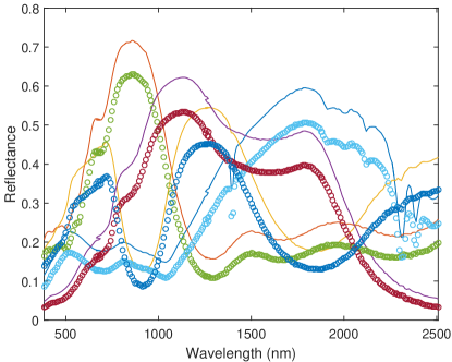
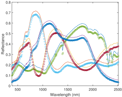
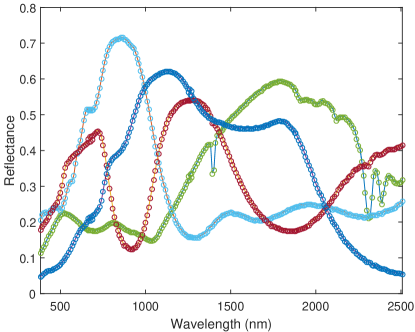
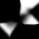
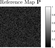
In order to build the endmember matrix ${\mathbf{E}}$, we have randomly selected four spectral signatures from the United States Geological Survey (USGS) digital spectral library. In this experiment, the number of endmembers is fixed to $m=4$ and the reflectance spectra have $L=224$ spectral bands ranging from $383$nm to $2508$nm. The ground-truth of the endmembers are displayed with solid lines in Fig. 1, 2 and 3. The abundance matrix ${\mathbf{A}}$ has been generated by drawing vectors distributed according to the uniform distribution in the simplex ${\mathcal{A}}$ defined by the non-negativity and sum-to-one constraints. The generated ground-truth of the abundance maps are shown in the first row of Figs. 4. The values of $P$ for all pixels have been generated by drawing samples from a uniform distribution on $[0,1]$ and is shown in the top left of Figs. 5. Unless indicated, the performance of these algorithms has been evaluated on a synthetic data of size $100\times 100\times 224$ whose signal to noise ratio (SNR) has been fixed to SNR=$40$dB.

III-B1 Initialization

For the proposed method, the initializations of ${\mathbf{E}}$ and ${\mathbf{P}}$ are necessary. The endmember signatures have been initialized by using the outputs of the VCA algorithm [18], which is one of the state-of-the-art endmember extraction methods. The reference endmembers and their estimates provided by the VCA algorithm are displayed in Fig. 1 (right). The matrix ${\mathbf{P}}$ is initialized with the zero matrix.

Figure 1: Actual endmembers (solid lines) and their estimates with VCA (circles).

III-B2 Stopping rule

As all the constraints associated with the endmembers and abundances are guaranteed to be satisfied at each update, the main issue after several updates is to analyze the value of the objective function. The stopping rule used in our experiments is defined as

$$\begin{split}&L({\mathbf{E}},{\mathbf{A}},{\mathbf{P}})<\eta_{1}\quad\textrm{ or }\\ &\frac{L({\mathbf{E}}^{(t)},{\mathbf{A}}^{(t)},{\mathbf{P}}^{(t)})-L({\mathbf{E}}^{(t-1)},{\mathbf{A}}^{(t-1)},{\mathbf{P}}^{(t-1)})}{L({\mathbf{E}}^{(t-1)},{\mathbf{A}}^{(t-1)},{\mathbf{P}}^{(t-1)})}<\eta_{2}\end{split}$$

where $\eta_{1}=n\sigma^{2}$ (product of the number of pixels $n$ and the noise power $\sigma^{2}$) and $\eta_{2}$ has been fixed to $10^{-3}$ by cross validation.

III-B3 Unmixing Results

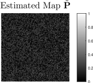
The estimated endmember matrices, abundance maps and probability matrix are reported in Figs. 3, 4 and 5. To further illustrate the role of nonlinear unmixing, we have compared our results with an LMM-based strategy. To achieve this, we simply fixed ${\mathbf{P}}=\bm{0}$, leading to an unsupervised LMM spectral unmixing method. The estimated endmembers are plotted in Fig. 2 and the abundance maps are included in Fig. 4. By fixing the endmember matrix ${\mathbf{E}}$ to the VCA estimates, we obtain the supervised versions of the algorithms for linear and nonlinear unmixing. To simplify the notations, linear and nonlinear unmixing are referred to as LU and NLU thereafter. Note that the supervised NLU can be regarded as a variant of Heylen’s method in [1] with the additional constraint that the elements of ${\mathbf{P}}$ belong to $[0,1]$. Quantitative results for the estimated endmembers and abundances for both LU and NLU are reported in Table I.

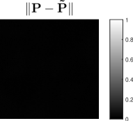
Figs. 1, 2 and 3 show that the unsupervised unmixing methods (linear and nonlinear) improve the estimation accuracy of the endmember signatures significantly compared to the output of VCA. This result demonstrates the necessity of updating ${\mathbf{E}}$ jointly with the other parameters ${\mathbf{A}}$ and ${\mathbf{P}}$. Furthermore, as shown in Figs. 2 and 3, the estimated endmembers using NLU are much closer to the ground-truth than their counterparts obtained using LU. The same conclusion holds for the estimation of abundances as shown in Fig. 4. These results are further confirmed in the quantitative results reported in Table. I. The values of $P$ obtained for all pixels are displayed in Fig. 5 and can be used to assess the importance of nonlinear effects, which matches the ground-truth quite well.

Figure 2: Actual endmembers (solid lines) and their estimates using the unsupervised LU method (circles).

Figure 3: Actual endmembers (solid lines) and their estimates using the unsupervised NLU method (circles).

Ground-truth

Supervised LU

Unsupervised LU

Supervised NLU

Unsupervised NLU

Figure 4: Abundance maps: ground-truth (line 1), estimation by supervised LU (line 2), unsupervised LU (line 3), supervised NLU (line 4) and unsupervised NLU (line 5).

Figure 5: Probability estimation: ground-truth ${\mathbf{P}}$ (top left), estimated $\tilde{{\mathbf{P}}}$ (top right) and their difference $\|{\mathbf{P}}-\tilde{{\mathbf{P}}}\|$ (bottom).

TABLE I: Comparison of Unmixing Performance for Synthetic datasets: SAM_E (in degree), NMSE_E (in dB), NMSE_A (in dB) and NMSE_P (in dB).

Methods	SAME	NMSEE	NMSEA	NMSEP
LU (fixing ${\mathbf{E}}$)	2.42	-14.72	-24.37	/
LU (relaxing ${\mathbf{E}}$)	2.08	-21.09	-24.38	/
NLU (fixing ${\mathbf{E}}$)	2.42	-14.72	-26.52	-0.035
NLU (relaxing ${\mathbf{E}}$)	0.13	-44.05	-48.77	-25.26

III-C Real Dataset

III-C1 Tahoe Dataset

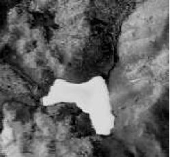
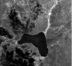
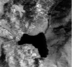
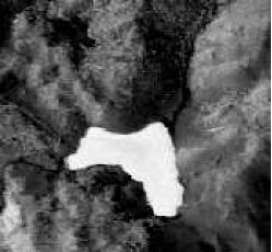
In this experiment, we consider an HS image of size $161\times 174\times 224$ acquired over Tahoe, located along the border between California and Nevada, on October 13th, 2015 by the JPL/NASA airborne visible/infrared imaging spectrometer (AVIRIS). This image was initially composed of $224$ bands that have been reduced to $192$ bands ($d=192$) after removing the water vapor absorption bands as well as the highly noisy bands. The spatial resolution of this HS image is around $20$m per pixel and it mainly contains water, soil and vegetation. A composite color image of the scene of interest is shown in the left of Fig. 6. In this experiment, the number of endmembers is fixed to be $m=3$ according to our available prior knowledge. The three endmembers were estimated using VCA and are shown with solid lines in Fig. 7. Note that ${\mathbf{P}}=\bm{0}$ was used for the initialization of ${\mathbf{P}}$ as in Section III-B.

Figure 6: Left: Tahoe dataset. Middle: Estimated map $\hat{{\mathbf{P}}}$. Right: Sum of absolute differences between abundance maps estimated by LU and NLU.

Figure 7: Tahoe dataset: Estimated endmember signatures of soil, vegetation and water using (Top) VCA (solid) and LU (circle), (Bottom) VCA (solid) and NLU (circle).

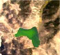
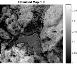
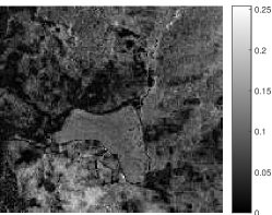
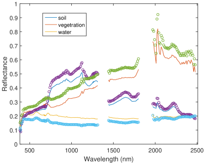
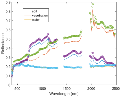
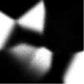
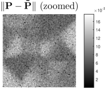
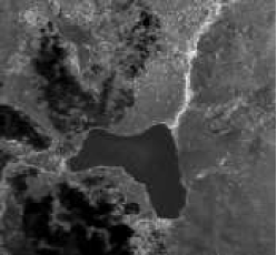
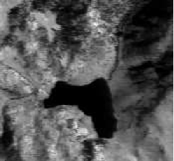
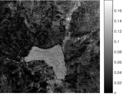
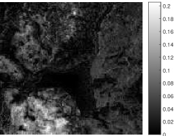
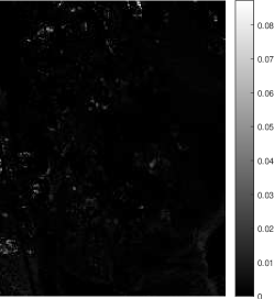
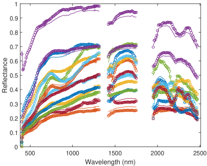
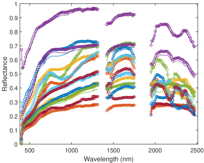
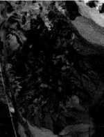
The proposed NLU and LU (obtained by fixing ${\mathbf{P}}=\bm{0}$) have been implemented to process the observed image. As there is no ground-truth for this image, unmixing results are first studied qualitatively by displaying the endmembers and abundances. Figs. 7 show that the the estimated signatures of soil and vegetation using LU and NLU are similar while those of water are slightly different. The corresponding abundance maps obtained by LU and NLU shown in the first two rows of Figs. 8 (the color scales are exactly the same) are globally similar. However, some differences can be observed in the last row of Fig. 8. It is interesting to note that the abundance maps of NLU have larger contrast than the ones obtained with LU, which is usually expected for good unmixing results. For example, the lake part is expected to have small values in the abundance map of soil and to have big values in abundance map of water. As is shown in the first and second rows of Figs. 8, the lake part in NLU is darker than the one in LU for the soil map and is brighter than the one in LU for the water map, showing that the results obtained by NLU consist more reasonably with our experience. In order to appreciate the interest of using a nonlinear unmixing strategy, Fig. 6 shows the estimated map of ${\mathbf{P}}$ (in the middle) which reflects the distribution of nonlinearity and the sum of absolute differences between abundance maps estimated by LU and NLU. It is interesting to note that the areas with large differences in abundance maps accord well with the areas associated with large values of ${\mathbf{P}}$. In these shared areas, nonlinear effects can be expected as there exist multiple interactions between endmembers in the ridge of mountain, in the shadow of mountain in the lake, etc.

Unsupervised LU

Unsupervised NLU

Difference

Figure 8: Estimated abundance maps with LU and NLU methods (from left to right): soil, vegetation and water.

III-C2 Cuprite Dataset

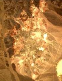
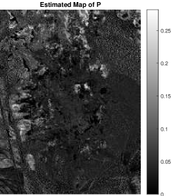
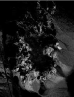
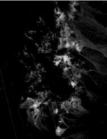
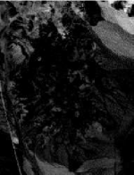
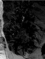
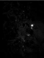
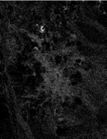
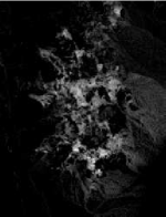
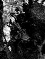
This section investigates the performance of the proposed NLU method for unmixing the well-known Cuprite HS image. This image, which has received a lot of interest in the remote sensing and geoscience literature, was acquired over Cuprite field by AVIRIS. It corresponds to a mining area in southern Nevada composed of several minerals and some vegetation, located approximately $200$km northwest of Las Vegas. The image considered in this experiment consists of $250\times 191$ pixels of $n_{\lambda}=188$ spectral bands obtained after removing the water vapor absorption bands. A composite color image of the scene of interest is shown in the left of Fig. 9. According to [18], the number of endmembers has been set to $m=14$. The estimated endmember signatures from VCA, LU and NLU are displayed in Fig. 10 and the $m=14$ corresponding abundance maps estimated using LU and NLU are shown in Figs. 11 and 12. Visually, VCA, LU and NLU provide similar endmembers and abundance maps. The estimated map of probability ${\mathbf{P}}$ from NLU and the differences between the estimated LU and NLU abundance maps are shown in Figs. 9 (middle and right). Again, the areas with large differences in the abundance maps overlap with the ones with large nonlinear effects. Nonlinear effects can be expected in this scenario as there exist intimate mixtures, in which a light ray can interact many times with the different mineral grains.

Figure 9: Left: Cuprite dataset. Middle: Estimated map $\hat{{\mathbf{P}}}$. Right: Sum of absolute differences between abundance maps estimated by LU and NLU.

Figure 10: Cuprite dataset: Extracted endmember signatures using (Top) VCA (solid) and LU (circle), (Bottom) VCA (solid) and NLU (circle).

(a) Alunite

(b) Sphene

(c) Andradite

(d) Muscovite

(e) Kaolinite #1

(f) Nontronite

(g) Kaolinite #4

(h) Kaolinite #3

(i) Pyrope #2

(j) Buddingtonite

(k) Montmorillonite

(l) Pyrope #1

(m) Kaolinite #2

(n) Dumortierite

Figure 11: Cuprite dataset: abundance maps estimated by LU.

(a) Alunite

(b) Sphene

(c) Andradite

(d) Muscovite

(e) Kaolinite #1

(f) Nontronite

(g) Kaolinite #4

(h) Kaolinite #3

(i) Pyrope #2

(j) Buddingtonite

(k) Montmorillonite

(l) Pyrope #1

(m) Kaolinite #2

(n) Dumortierite

Figure 12: Cuprite dataset: abundance maps estimated by NLU.

IV Conclusion

This paper studied a new unsupervised nonlinear spectral unmixing method based on a recent multilinear model. The nonlinear unmixing problem was formulated as a constrained optimization problem with respect to the endmembers, abundances and pixel-dependant transition probabilities. A gradient projection within block coordinate descent method was proposed to estimate these three sets of variables jointly. Each step of the proposed method was carefully addressed to guarantee the convergence to a stationary point of the objective function. Experiments implemented on both synthetic and real datasets confirmed that the multilinear model based nonlinear unmixing allows us to detect and analyze the non-linearities present in a hyperspectral image. Further work will be devoted to investigate a similar nonlinear unmixing algorithm accounting for spatial correlations for the abundances and the transition probabilities.

References

- [1] R. Heylen and P. Scheunders, “A multilinear mixing model for nonlinear spectral unmixing,” IEEE Trans. Geosci. Remote Sens., vol. 54, no. 1, pp. 240–251, Jan 2016.
- [2] A. Averbuch, M. Zheludev, and V. Zheludev, “Unmixing and target recognition in hyper-spectral imaging,” Earth Science Research, vol. 1, no. 2, pp. 200–228, 2012.
- [3] K. E. Themelis, F. Schmidt, O. Sykioti, A. A. Rontogiannis, K. D. Koutroumbas, and I. A. Daglis, “On the unmixing of MEx/OMEGA hyperspectral data,” Planetary and Space Science, vol. 68, no. 1, pp. 34–41, 2012.
- [4] N. Dobigeon and N. Brun, “Spectral mixture analysis of EELS spectrum-images,” Ultramicroscopy, vol. 120, pp. 25–34, Sept. 2012.
- [5] C. Carteret, A. Dandeu, S. Moussaoui, H. Muhr, B. Humbert, and E. Plasari, “Polymorphism studied by lattice phonon raman spectroscopy and statistical mixture analysis method. Application to calcium carbonate polymorphs during batch crystallization,” Crystal Growth & Design, vol. 9, no. 2, pp. 807–812, 2009.
- [6] Y. Huang, A. K. Zaas, A. Rao, N. Dobigeon, P. J. Woolf, T. Veldman, N. C. Oien, M. T. McClain, J. B. Varkey, B. Nicholson, L. Carin, S. Kingsmore, C. W. Woods, G. S. Ginsburg, and A. Hero, “Temporal dynamics of host molecular responses differentiate symptomatic and asymptomatic influenza A infection,” PLoS Genetics, vol. 8, no. 7, p. e1002234, Aug. 2011.
- [7] C.-I Chang, X.-L. Zhao, M. L. G. Althouse, and J. J. Pan, “Least squares subspace projection approach to mixed pixel classification for hyperspectral images,” IEEE Trans. Geosci. Remote Sens., vol. 36, no. 3, pp. 898–912, May 1998.
- [8] J. Wang and C.-I Chang, “Applications of independent component analysis in endmember extraction and abundance quantification for hyperspectral imagery,” IEEE Trans. Geosci. Remote Sens., vol. 4, no. 9, pp. 2601–2616, Sept. 2006.
- [9] D. Manolakis, C. Siracusa, and G. Shaw, “Hyperspectral subpixel target detection using the linear mixing model,” IEEE Trans. Geosci. Remote Sens., vol. 39, no. 7, pp. 1392–1409, July 2001.
- [10] N. Keshava and J. F. Mustard, “Spectral unmixing,” IEEE Signal Process. Mag., vol. 19, no. 1, pp. 44–57, Jan. 2002.
- [11] R. A. Horn and C. R. Johnson, Matrix analysis. Cambridge, UK: Cambridge university press, 2012.
- [12] N. Dobigeon, J.-Y. Tourneret, C. Richard, J. C. M. Bermudez, S. McLaughlin, and A. O. Hero, “Nonlinear unmixing of hyperspectral images: Models and algorithms,” IEEE Signal Process. Mag., vol. 31, no. 1, pp. 89–94, Jan. 2014.
- [13] B. Hapke, “Bidirectional reflectance spectroscopy: 1. theory,” J. Geophys. Res., vol. 86, no. B4, pp. 3039–3054, Apr. 1981.
- [14] A. Halimi, Y. Altmann, N. Dobigeon, and J.-Y. Tourneret, “Nonlinear unmixing of hyperspectral images using a generalized bilinear model,” IEEE Trans. Geosci. Remote Sens., vol. 49, no. 11, pp. 4153–4162, 2011.
- [15] N. Yokoya, J. Chanussot, and A. Iwasaki, “Nonlinear unmixing of hyperspectral data using semi-nonnegative matrix factorization,” IEEE Trans. Geosci. Remote Sens., vol. 52, no. 2, pp. 1430–1437, 2014.
- [16] I. Meganem, P. Deliot, X. Briottet, Y. Deville, and S. Hosseini, “Linear–quadratic mixing model for reflectances in urban environments,” IEEE Trans. Geosci. Remote Sens., vol. 52, no. 1, pp. 544–558, 2014.
- [17] Y. Altmann, A. Halimi, N. Dobigeon, and J.-Y. Tourneret, “Supervised nonlinear spectral unmixing using a postnonlinear mixing model for hyperspectral imagery,” IEEE Trans. Image Process., vol. 21, no. 6, pp. 3017–3025, June 2012.
- [18] J. Nascimento and J. Bioucas-Dias, “Vertex component analysis: A fast algorithm to unmix hyperspectral data,” IEEE Trans. Geosci. Remote Sens., vol. 43, no. 4, pp. 898–910, 2005.
- [19] D. P. Bertsekas, Nonlinear programming. Athena Scientific, 1999.
- [20] M. Pereyra, P. Schniter, E. Chouzenoux, J.-C. Pesquet, J.-Y. Tourneret, A. Hero, and S. Mclaughlin, “A survey of stochastic simulation and optimization methods in signal processing,” IEEE J. Sel. Topics Signal Process., vol. 10, no. 2, pp. 224–241, March 2016.
- [21] D. C. Heinz and C.-I. Chang, “Fully constrained least squares linear spectral mixture analysis method for material quantification in hyperspectral imagery,” IEEE Trans. Geosci. Remote Sens., vol. 39, no. 3, pp. 529–545, 2001.
- [22] S. Boyd, N. Parikh, E. Chu, B. Peleato, and J. Eckstein, “Distributed optimization and statistical learning via the alternating direction method of multipliers,” Foundations and Trends® in Machine Learning, vol. 3, no. 1, pp. 1–122, 2011.
- [23] J. M. Bioucas-Dias and M. A. Figueiredo, “Alternating direction algorithms for constrained sparse regression: Application to hyperspectral unmixing,” in Proc. IEEE GRSS Workshop Hyperspectral Image SIgnal Process.: Evolution in Remote Sens. (WHISPERS), Reykjavik, Iceland, Jun. 2010, pp. 1–4.
- [24] Q. Wei, J. Bioucas-Dias, N. Dobigeon, and J.-Y. Tourneret, “Fast spectral unmixing based on Dykstra’s alternating projection,” IEEE Trans. Signal Process., submitted.
- [25] P. H. Calamai and J. J. Moré, “Projected gradient methods for linearly constrained problems,” Math. Progam., vol. 39, no. 1, pp. 93–116, 1987.
- [26] P. L. Combettes and V. R. Wajs, “Signal recovery by proximal forward-backward splitting,” Multiscale Modeling & Simulation, vol. 4, no. 4, pp. 1168–1200, 2005.
- [27] C. Michelot, “A finite algorithm for finding the projection of a point onto the canonical simplex of ,” J. Optimization Theory Applications, vol. 50, no. 1, pp. 195–200, 1986.
- [28] J. Duchi, S. Shalev-Shwartz, Y. Singer, and T. Chandra, “Efficient projections onto the for learning in high dimensions,” in Proc. Int. Conf. Machine Learning (ICML), Helsinki, Finland, 2008, pp. 272–279.
- [29] L. Condat, “Fast projection onto the simplex and the l1 ball,” Hal preprint: hal-01056171, 2014.
- [30] A. Beck and L. Tetruashvili, “On the convergence of block coordinate descent type methods,” SIAM J. Optim., vol. 23, no. 4, pp. 2037–2060, 2013.
- [31] J. Bolte, S. Sabach, and M. Teboulle, “Proximal alternating linearized minimization for nonconvex and nonsmooth problems,” Math. Progam., vol. 146, no. 1-2, pp. 459–494, 2014.
- [32] S. J. Wright, “Coordinate descent algorithms,” Math. Progam., vol. 151, no. 1, pp. 3–34, 2015.
- [33] E. Chouzenoux, J.-C. Pesquet, and A. Repetti, “A block coordinate variable metric forward-backward algorithm,” 2013.