Aller guten Dinge sind drei: Cosmology with three interacting spin-2 fields

Abstract

Theories of massive gravity with one or two dynamical metrics generically lack stable and observationally-viable cosmological solutions that are distinguishable from $\Lambda$CDM. We consider an extension to trimetric gravity, with three interacting spin-2 fields which are not plagued by the Boulware-Deser ghost. We systematically explore every combination with two free parameters in search of background cosmologies that are competitive with $\Lambda$CDM. For each case we determine whether the expansion history satisfies viability criteria, and whether or not it contains beyond-$\Lambda$CDM phenomenology. Among the many models we consider, there are only three cases that seem to be both viable and distinguishable from standard cosmology. One of the models has only one free parameter and displays a crossing from above to below the phantom divide. The other two provide scaling behavior, although they contain future singularities that need to be studied in more detail. These models possess interesting features that make them compelling targets for a full comparison to observations of both cosmological expansion history and structure formation.

I Introduction

The past half-decade has borne witness to a revolution in our understanding of the physics of spin-2 fields. While it has been known for decades that the unique theory describing a massless spin-2 field is general relativity Gupta (1954); Weinberg (1965); Deser (1970); Boulware and Deser (1975); Feynman (1996), it had similarly been a long-standing belief that massive and interacting spin-2 fields were generically plagued by the nonlinear Boulware-Deser ghost Boulware and Deser (1972), despite admitting a healthy linear formulation Fierz and Pauli (1939). This story was turned on its head when, building on earlier work in Refs. Arkani-Hamed et al. (2003); Creminelli et al. (2005), de Rham, Gabadadze, and Tolley (dRGT) constructed a theory of a massive graviton de Rham and Gabadadze (2010); de Rham et al. (2011a) which has been shown through a variety of methods to be free of the Boulware-Deser mode Hassan and Rosen (2011, 2012a); de Rham et al. (2012, 2011b); Hassan et al. (2012a); Hassan and Rosen (2012b); Hassan et al. (2012b); Hinterbichler and Rosen (2012).

The breakthrough in massive gravity led to a corresponding advance in theories of multiple interacting gravitons, or, equivalently, multiple metrics. The dRGT construction contains two metrics, a spacetime metric and a fixed reference metric which must be inserted by hand (typically chosen to be that of Minkowski space). By promoting this fixed metric to a dynamical one, one arrives at a theory of bimetric gravity (or bigravity) which is also ghost-free Hassan and Rosen (2012c). Theories describing multiple metrics can be trivially constructed from here by coupling various pairs of metrics in the same manner as in bigravity, using the ghost-free potential. These theories also avoid the Boulware-Deser ghost Hinterbichler and Rosen (2012), up to certain conditions on which we elaborate below Nomura and Soda (2012); Scargill et al. (2014); de Rham and Tolley (2015); de Rham et al. (2015a).

With theoretically-consistent theories in hand, the next step is to search for physical solutions. Given that multimetric theories are fundamentally theories of massive gravitons in addition to a massless one—generically a theory of $n$ metrics contains $n-1$ massive gravitons and one massless one, of which matter couples to some combination—they modify general relativity predominantly at large distances, i.e., they are infrared modifications to gravity. As it turns out, general relativity has a well-known and significant problem in reconciling theory and observation at cosmological distances (see, e.g., Ref. Bull et al. (2016)): the accelerating Universe Riess et al. (1998); Perlmutter et al. (1999), which naturally lends itself to solutions involving modifying gravity on large scales Clifton et al. (2012). It is therefore entirely natural to ask whether massive gravity or its multimetric generalizations can solve this problem.

There are two immediately necessary (though not sufficient) criteria for a modified-gravity theory to successfully address the accelerating Universe. First, it needs to have cosmological solutions which self-accelerate, i.e., which possess late-time acceleration in the absence of dark energy. Second, it needs to have stable fluctuations about these self-accelerating solutions. Unfortunately, this has proven rather difficult to achieve in massive gravity and bigravity. In the simplest massive gravity case, in which the reference metric is flat space, spatially-flat and closed Friedmann-Lemaître-Robertson-Walker (FLRW) solutions do not exist D’Amico et al. (2011). Solutions can be obtained by considering open FLRW or more general reference metrics, but these solutions seem to generically contain instabilities Gümrükçüoğlu et al. (2011, 2012); Vakili and Khosravi (2012); De Felice et al. (2012); Fasiello and Tolley (2012); De Felice et al. (2013). In bigravity, the situation is slightly improved, as it is not difficult to find FLRW solutions that agree with observations of the cosmic expansion history Volkov (2012); Comelli et al. (2012a); von Strauss et al. (2012); Akrami et al. (2013a, b); Könnig et al. (2014a); Enander et al. (2015a). However, linear perturbations, studied extensively in Refs. Comelli et al. (2012b); Khosravi et al. (2012a); Berg et al. (2012); Könnig and Amendola (2014); Solomon et al. (2014); Könnig et al. (2014b); Lagos and Ferreira (2014); Cusin et al. (2015); Yamashita and Tanaka (2014); De Felice et al. (2014); Fasiello and Tolley (2013); Enander et al. (2015b); Amendola et al. (2015); Johnson and Terrana (2015); Könnig (2015), tend to contain either ghost or gradient instabilities. In each of these cases there are potential ways out. In massive gravity, one might consider large-scale inhomogeneities D’Amico et al. (2011). In bigravity, cosmological solutions can be made stable back to arbitrarily early times by taking one Planck mass to be much smaller than the other Akrami et al. (2015), or by reintroducing a cosmological constant which is much larger than the bimetric interaction parameter Könnig and Amendola (2014). It is also possible that the gradient instability in bigravity is cured at the nonlinear level Mortsell and Enander (2015) due to a version of the Vainshtein screening mechanism Vainshtein (1972); Babichev and Deffayet (2013). However, there remains strong motivation to find a massive gravity or multigravity theory with self-accelerating solutions that are linearly stable at all times.

One logical step in this direction is to inquire what happens cosmologically if we have three, rather than two, interacting spin-2 fields. This generalization has been discussed before in Refs. Khosravi et al. (2012b); Tamanini et al. (2014); Scargill et al. (2014), but all the cases studied in those references are pathological. Ref. Khosravi et al. (2012b) studied a theory of massive trimetric gravity where all three metrics interact with each other directly, making a cycle of interactions; as we will discuss in the next section, such theories are plagued by the Boulware-Deser ghost Nomura and Soda (2012). Ref. Tamanini et al. (2014), on the other hand, studied a multigravitational theory in terms of vierbeins with no metric formulation. Such theories turned out later to also suffer from the Boulware-Deser ghost. Ref. Scargill et al. (2014) compares multimetric models in the metric and vierbein formalism, but does not look at cosmological solutions, while Ref. Baldacchino and Schmidt-May (2016) examines maximally-symmetric solutions in multigravity.

In this paper, we consider the cosmologies of healthy theories of trigravity and scan various models by examining a large number of combinations of parameters in search for interesting background cosmological solutions. Here, “interesting” means cosmological solutions that are both viable and qualitatively different from those occurring in bigravity. Appropriate perturbative analyses of the interesting models will then be required to see whether any of them could be free from instabilities; we leave this for future work.

We note that this paper examines a number of trimetric models in detail and is therefore fairly lengthy. The especially busy reader is directed to section V for a summary of “positive” results. An overview with an additional level of detail can be found in tables 1 and 2, where we present various cosmological viability criteria for all of the models studied.

II The theory of massive trigravity

We begin by presenting the theory of massive trimetric gravity, or trigravity, describing three interacting spin-2 fields in four dimensions. We will work in the metric formulation of trigravity, in which the spin-2 fields are described by three metric-like tensors.

How should the three metrics couple to each other? When metrics interact, the Boulware-Deser ghost looms as a nearly-inevitable pitfall, and extreme caution must be taken to avoid it. Fortunately, as mentioned in the previous secion, the interaction potentials which avoid this ghost are known and have been formulated in the context of massive gravity and bigravity. This provides an immediate avenue for trimetric gravity: we could couple each pair of metrics via the ghost-free potential, leading to a cycle of interactions. However, such cycles turn out to be plagued by the Boulware-Deser ghost Nomura and Soda (2012); Scargill et al. (2014); de Rham and Tolley (2015). Therefore we are forced to consider breaking the cycle into a line, i.e., there must be one pair of metrics which do not directly interact with each other.

Next we must consider how these metrics couple to matter. In the simpler cases of massive gravity and bigravity, where there are two metrics rather than three, the question of how matter couples was the source of much discussion and debate Hassan and Rosen (2012c); Hassan et al. (2013); Akrami et al. (2013c); Tamanini et al. (2014); Akrami et al. (2014); Yamashita et al. (2014); de Rham et al. (2015b, b); Hassan et al. (2014); Enander et al. (2015a); Solomon et al. (2015); Schmidt-May (2015); de Rham et al. (2014); Gümrükçüoğlu et al. (2015a); Heisenberg (2015a); Gümrükçüoğlu et al. (2015b); Hinterbichler and Rosen (2015); Heisenberg (2015b, c); Lagos and Noller (2016); Melville and Noller (2016), leading to the conclusion that the Boulware-Deser ghost almost always re-emerges if any matter field couples to more than one metric, or if matter coupled to one metric interacts with matter coupled to another. We will therefore take all matter to couple minimally to a single metric, which we will call $g$. Because matter moves on geodesics of this metric, we can interpret it as the physical metric describing the geometry of spacetime, exactly like in general relativity. The other two metrics, which we will denote as $f_{1}$ and $f_{2}$ (or $f_{1,\mu\nu}$ and $f_{2,\mu\nu}$), couple only to each other or to $g$, and thus are responsible for modifying gravity.

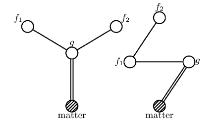
This leaves us with two different classes of ghost-free trimetric theory. In the first, the metrics $f_{1}$ and $f_{2}$ both couple to the physical metric $g$, but not to each other. We will call this star trigravity. The other possibility is to couple one of the additional metrics, without loss of generality $f_{1}$, to each of the other metrics, $g$ and $f_{2}$. In this theory, which we call path trigravity, there is no coupling between $g$ and $f_{2}$. The two theories are depicted schematically in fig. 1. In the rest of this section, we proceed with discussing both classes of trigravity in full detail and generality, before moving on with studying the background cosmology of the two theories in the next sections.

Figure 1: Visual depiction of star trigravity (left) and path trigravity (right). The white circles and the single lines between them represent, respectively, the three metrics and the interaction terms mixing them. The shaded circles and the double lines represent the matter fields and their couplings to the physical metric, $g$, respectively.

II.1 Star trigravity

In star trigravity, $g_{\mu\nu}$ couples to $f_{1,\mu\nu}$, $f_{2,\mu\nu}$, as well as all matter fields, $\Phi$. The action is given by

$$S =-\frac{M_{\mathrm{Pl}}^{2}}{2}\int\mathrm{d}^{4}x\sqrt{-\det g}R(g)-\sum_{i=1}^{2}\frac{M_{i}^{2}}{2}\int\mathrm{d}^{4}x\sqrt{-\det f_{i}}R(f_{i})$$

$$+\sum_{i=1}^{2}m_{i}^{2}M_{\mathrm{Pl}}^{2}\int\mathrm{d}^{4}x\sqrt{-\det g}\sum_{n=0}^{4}\beta_{i,n}e_{n}\Bigl{(}\sqrt{g^{-1}f_{i}}\Bigr{)}+\int\mathrm{d}^{4}x\sqrt{-\det g}\mathcal{L}_{\text{m}}(g,\Phi),$$ (1)

where $\sqrt{g^{-1}f_{i}}$ is the matrix square root of $g^{\mu\rho}f_{i,\rho\nu}$, the $e_{n}$ are the elementary symmetric polynomials of the eigenvalues of the square-root matrix, as presented in, e.g., Ref. Hassan and Rosen (2012c), and $\beta_{i,n}$ are the dimensionless coupling constants for the interactions between $g_{\mu\nu}$ and $f_{i,\mu\nu}$. The first index $i$ corresponds to the metric $f_{i,\mu\nu}$ involved in the interaction with the physical metric $g_{\mu\nu}$, while the second index $n$ specifies the order of the interaction and can take the values $n=\{0,...,4\}$. $M_{\mathrm{Pl}}$ and $M_{i}$ are the Planck masses and $R(g)$ and $R(f_{i})$ are the Ricci scalars for the metrics $g_{\mu\nu}$ and $f_{i,\mu\nu}$, respectively. This theory is symmetric under the interchange of the metrics $f_{1}$ and $f_{2}$, along with their Planck masses and interaction parameters. The two mass parameters $m_{i}^{2}$ can be absorbed into the $\beta_{i,n}$, so that the $\beta_{i,n}$ will have dimensions of mass squared.

The two Planck masses of $f_{i,\mu\nu}$, $M_{i}$, are redundant parameters and can be set equal to $M_{\mathrm{Pl}}$. To see this, consider the rescaling $f_{i,\mu\nu}\rightarrow(M_{\mathrm{Pl}}/M_{i})^{2}f_{i,\mu\nu}$. The Ricci scalars $R(f_{i})$ transform as $R(f_{i})\rightarrow(M_{\mathrm{Pl}}/M_{i})^{2}R(f_{i})$, so the corresponding Einstein-Hilbert terms in the action become

$$\frac{M_{i}^{2}}{2}\sqrt{-\det f_{i}}R(f_{i})\rightarrow\frac{M_{\mathrm{Pl}}^{2}}{2}\sqrt{-\det f_{i}}R(f_{i}).$$ (2)

In addition to the Einstein-Hilbert terms, the interaction terms in the action also depend on $f_{i,\mu\nu}$. These transform as

$$\sum_{n=0}^{4}\beta_{i,n}e_{n}\Bigl{(}\sqrt{g^{-1}f_{i}}\Bigr{)}\rightarrow\sum_{n=0}^{4}\beta_{i,n}e_{n}\left(\frac{M_{\mathrm{Pl}}}{M_{i}}\sqrt{g^{-1}f_{i}}\right)=\sum_{n=0}^{4}\beta_{i,n}\left(\frac{M_{\mathrm{Pl}}}{M_{i}}\right)^{n}e_{n}\Bigl{(}\sqrt{g^{-1}f_{i}}\Bigr{)},$$ (3)

where in the last equality we used the scaling properties of the elementary polynomials $e_{n}(\mathbb{X})$. Redefining the interaction couplings as $\beta_{i,n}\rightarrow(M_{i}/M_{\mathrm{Pl}})^{n}\beta_{i,n}$, we end up with the original star trigravity action, but with $M_{1}=M_{2}=M_{\mathrm{Pl}}$.

Variation of the action (1) with respect to $g_{\mu\nu}$ and $f_{i,\mu\nu}$ yields the modified Einstein equations for the metrics (after absorbing $m_{i}^{2}$ into $\beta_{i,n}$ and seting $M_{i}=M_{\mathrm{Pl}}$),

$$G_{\mu\nu}+\sum_{i=1}^{2}\sum_{n=0}^{3}(-1)^{n}\beta_{i,n}g_{\mu\lambda}Y_{(n)\nu}^{\lambda}\Bigl{(}\sqrt{g^{-1}f_{i}}\Bigr{)} =\frac{1}{M_{\mathrm{Pl}}^{2}}T_{\mu\nu},$$ (4)

$$G_{i,\mu\nu}+\sum_{n=0}^{3}(-1)^{n}\beta_{i,4-n}f_{i,\mu\lambda}Y_{(n)\nu}^{\lambda}\Bigl{(}\sqrt{f_{i}^{-1}g}\Bigr{)} =0,$$ (5)

where $G_{\mu\nu}$ and $G_{i,\mu\nu}$ are the Einstein tensors of $g_{\mu\nu}$ and $f_{i,\mu\nu}$, respectively, and $T_{\mu\nu}$ is the stress-energy tensor defined with respect to $g_{\mu\nu}$ as $T_{\mu\nu}\equiv-\frac{2}{\sqrt{-\det g}}\frac{\delta\left(\sqrt{-\det g}\mathcal{L}_{\mathrm{m}}\right)}{\delta g^{\mu\nu}}$. The matrices $Y_{(n)}(\mathbb{X})$ for a matrix $\mathbb{X}$ are defined as

$$Y_{(0)}(\mathbb{X}) \equiv\mathbb{I},\quad$$

$$Y_{(1)}(\mathbb{X}) \equiv\mathbb{X}-\mathbb{I}[\mathbb{X}],\quad$$

$$Y_{(2)}(\mathbb{X}) \equiv\mathbb{X}^{2}-\mathbb{X}[\mathbb{X}]+\frac{1}{2}\mathbb{I}\left([\mathbb{X}]^{2}-[\mathbb{X}^{2}]\right),$$

$$Y_{(3)}(\mathbb{X}) \equiv\mathbb{X}^{3}-\mathbb{X}^{2}[\mathbb{X}]+\frac{1}{2}\mathbb{X}\left([\mathbb{X}]^{2}-[\mathbb{X}^{2}]\right)-\frac{1}{6}\mathbb{I}\left([\mathbb{X}]^{3}-3[\mathbb{X}][\mathbb{X}^{2}]+2[\mathbb{X}^{3}]\right),$$ (6)

where $\mathbb{I}$ is the identity matrix and $[...]$ is the trace operator.

Let us now consider the divergence of the Einstein equations (4) and (5). The Einstein tensors satisfy the Bianchi identities $\nabla^{\mu}G_{\mu\nu}=0$ and $\nabla_{i}^{\mu}G_{i,\mu\nu}=0$. General covariance of the matter sector implies conservation of the stress energy tensor, $\nabla^{\mu}T_{\mu\nu}=0$. Thus we are left with the Bianchi constraints,

$$\nabla^{\mu}\sum_{i=1}^{2}\sum_{n=0}^{3}(-1)^{n}\beta_{i,n}g_{\mu\lambda}Y_{(n)\nu}^{\lambda}\Bigl{(}\sqrt{g^{-1}f_{i}}\Bigr{)}=0,$$ (7)

$$\nabla_{i}^{\mu}\sum_{n=0}^{3}(-1)^{n}\beta_{i,4-n}f_{i,\mu\lambda}Y_{(n)\nu}^{\lambda}\Bigl{(}\sqrt{f_{i}^{-1}g}\Bigr{)}=0,$$ (8)

where $\nabla^{\mu}$ is the $g$-metric covariant derivative raised with respect to $g_{{\mu\nu}}$, and $\nabla_{i}^{\mu}$ are the corresponding operators for the $f_{i}$ metrics. These constraints arise from the fact that the ghost-free potentials are invariant under combined diffeomorphisms of the two metrics involved. They will be important in reducing some freedom in the cosmological solutions.

II.2 Path trigravity

In path trigravity, $g_{\mu\nu}$ couples directly to matter and to one of the reference metrics, which we choose to be $f_{1,\mu\nu}$. The latter couples in turn to $f_{2,\mu\nu}$. The action is therefore given by

$$S= -\frac{M_{\mathrm{Pl}}^{2}}{2}\int\mathrm{d}^{4}x\sqrt{-\det g}R(g)-\sum_{i=1}^{2}\frac{M_{i}^{2}}{2}\int\mathrm{d}^{4}x\sqrt{-\det f_{i}}R(f_{i})$$

$$+m_{1}^{2}M_{\mathrm{Pl}}^{2}\int\mathrm{d}^{4}x\sqrt{-\det g}\sum_{n=0}^{4}\beta_{1,n}e_{n}\Bigl{(}\sqrt{g^{-1}f_{1}}\Bigr{)}+m_{2}^{2}M_{\mathrm{Pl}}^{2}\sqrt{-\det f_{1}}\sum_{n=0}^{4}\beta_{2,n}e_{n}\Bigl{(}\sqrt{f_{1}^{-1}f_{2}}\Bigr{)}$$

$$+\int\mathrm{d}^{4}x\sqrt{-\det g}\mathcal{L}_{m}(g,\Phi),$$ (9)

with the same notations as in star trigravity, up to different definitions of the interaction parameters. Here the parameters $\beta_{1,n}$ describe the interactions between the physical metric $g_{\mu\nu}$ and the metric $f_{1,\mu\nu}$, while the $\beta_{2,n}$ describe the interactions between $f_{1,\mu\nu}$ and $f_{2,\mu\nu}$. In what follows, the two mass parameters $m_{i}^{2}$ will again be absorbed into the $\beta_{i,n}$.

Let us take a closer look at the $f_{i}$-metric Planck masses, $M_{i}$, which, as discussed in the context of star trigravity, are redundant parameters. Under the rescaling $f_{i,\mu\nu}\rightarrow(M_{\mathrm{Pl}}/M_{i})^{2}f_{i,\mu\nu}$, the Ricci scalars for $f_{1}$ and $f_{2}$ transform as above. Therefore, the Einstein-Hilbert terms transform as in eq. 2. However, the mass terms transform differently,

$$\sum_{n=0}^{4}\beta_{1,n}e_{n}\Bigl{(}\sqrt{g^{-1}f_{1}}\Bigr{)} \rightarrow\sum_{n=0}^{4}\beta_{1,n}e_{n}\Bigl{(}\frac{M_{\mathrm{Pl}}}{M_{1}}\sqrt{g^{-1}f_{1}}\Bigr{)}=\sum_{n=0}^{4}\beta_{1,n}\left(\frac{M_{\mathrm{Pl}}}{M_{1}}\right)^{n}e_{n}\Bigl{(}\sqrt{g^{-1}f_{1}}\Bigr{)},$$ (10)

$$\sum_{n=0}^{4}\beta_{2,n}e_{n}\Bigl{(}\sqrt{f_{1}^{-1}f_{2}}\Bigr{)} \rightarrow\sum_{n=0}^{4}\beta_{2,n}e_{n}\Bigl{(}\frac{M_{1}}{M_{2}}\sqrt{f_{1}^{-1}f_{2}}\Bigr{)}=\sum_{n=0}^{4}\beta_{2,n}\left(\frac{M_{1}}{M_{2}}\right)^{n}e_{n}\Bigl{(}\sqrt{f_{1}^{-1}f_{2}}\Bigr{)},$$ (11)

where we have again used the scaling properties of the elementary symmetric polynomials $e_{n}(\mathbb{X})$. By redefining the interaction parameters $\beta_{1,n}\rightarrow(M_{1}/M_{\mathrm{Pl}})^{n}\beta_{1,n}$ and $\beta_{2,n}\rightarrow(M_{2}/M_{1})^{n}\beta_{2,n}$ we end up with the original path trigravity action, but with $M_{1}=M_{2}=M_{\mathrm{Pl}}$. Therefore, we set $M_{i}=M_{\mathrm{Pl}}$ from now on.

Variation of the action (9) with respect to $g_{\mu\nu}$ and $f_{i,\mu\nu}$ yields the modified Einstein equations for the metrics,

$$G_{\mu\nu}+\sum_{n=0}^{3}(-1)^{n}\beta_{1,n}g_{\mu\lambda}Y_{(n)\nu}^{\lambda}\Bigl{(}\sqrt{g^{-1}f_{1}}\Bigr{)}=\frac{1}{M_{\mathrm{Pl}}^{2}}T_{\mu\nu},$$ (12)

$$G_{1,\mu\nu}+\sum_{n=0}^{3}(-1)^{n}\beta_{1,4-n}f_{1,\mu\lambda}Y_{(n)\nu}^{\lambda}\Bigl{(}\sqrt{f_{1}^{-1}g}\Bigr{)}+\sum_{n=0}^{3}(-1)^{n}\beta_{2,n}f_{1,\mu\lambda}Y_{(n)\nu}^{\lambda}\Bigl{(}\sqrt{f_{1}^{-1}f_{2}}\Bigr{)}=0,$$ (13)

$$G_{2,\mu\nu}+\sum_{n=0}^{3}(-1)^{n}\beta_{2,4-n}f_{2,\mu\lambda}Y_{(n)\nu}^{\lambda}\Bigl{(}\sqrt{f_{2}^{-1}f_{1}}\Bigr{)}=0,$$ (14)

where $G_{\mu\nu}$ and $G_{i,\mu\nu}$ are the Einstein tensors for $g_{\mu\nu}$ and $f_{i,\mu\nu}$, respectively. The matrices $Y_{(n)}$ are given by eq. 6 and $T_{\mu\nu}$ is the stress-energy tensor defined with respect to the physical metric $g$.

Let us take the covariant derivative of the Einstein equations (12)–(14). The Bianchi identities for $g_{\mu\nu}$, $f_{1,\mu\nu}$, and $f_{2,\mu\nu}$, and the covariant conservation of the stress-energy tensor lead to the Bianchi constraints

$$\nabla^{\mu}\sum_{n=0}^{3}(-1)^{n}\beta_{1,n}g_{\mu\lambda}Y_{(n)\nu}^{\lambda}\Bigl{(}\sqrt{g^{-1}f_{1}}\Bigr{)}=0,$$ (15)

$$\nabla_{1}^{\mu}\sum_{n=0}^{3}(-1)^{n}\beta_{1,4-n}f_{1,\mu\lambda}Y_{(n)\nu}^{\lambda}\Bigl{(}\sqrt{f_{1}^{-1}g}\Bigr{)}+\nabla_{1}^{\mu}\sum_{n=0}^{3}(-1)^{n}\beta_{2,n}f_{1,\mu\lambda}Y_{(n)\nu}^{\lambda}\Bigl{(}\sqrt{f_{1}^{-1}f_{2}}\Bigr{)}=0,$$ (16)

$$\nabla_{2}^{\mu}\sum_{n=0}^{3}(-1)^{n}\beta_{2,4-n}f_{2,\mu\lambda}Y_{(n)\nu}^{\lambda}\Bigl{(}\sqrt{f_{2}^{-1}f_{1}}\Bigr{)}=0.$$ (17)

As in star trigravity, these constraints will allow us to fix some otherwise-free variables.

III The background cosmology of trigravity

After having introduced the theories of star and path trigravity, we now turn to their cosmological solutions. We want to describe an isotropic and homogeneous universe, so we choose all our metrics to be of the FLRW form. This allows us to derive Friedmann equations for all the metrics. After further massaging, we can analyze the solutions to the Friedmann equations and find expressions for the matter density parameter and the effective equation of state.

We first study the background equations of star trigravity and then turn to the case of path trigravity, where we repeat the same procedure. The results of this section are general and hold for any choices of parameters.

III.1 Star trigravity

We assume that at the background level, the Universe is described by spatially-flat FLRW metrics for $g_{\mu\nu}$, $f_{1,\mu\nu}$, and $f_{2,\mu\nu}$,

$$\mathrm{d}s_{g}^{2} =a^{2}(-\mathrm{d}\tau^{2}+\mathrm{d}\vec{x}^{2}),$$ (18)

$$\mathrm{d}s_{f_{i}}^{2} =-N_{i}^{2}\mathrm{d}\tau^{2}+b_{i}^{2}\mathrm{d}\vec{x}^{2},$$ (19)

where $\tau$ is conformal time. The scale factor $a$ of $g_{\mu\nu}$ and the scale factors $b_{i}$ and lapses $N_{i}$ of $f_{i,\mu\nu}$ are functions of conformal time only. Since $g_{\mu\nu}$ is the physical metric that minimally couples to matter, its scale factor $a(\tau)$ is the observable scale factor, and similarly the cosmic time $t$ measured by observers is given by $\mathrm{d}t=a\mathrm{d}\tau$. Plugging these ansätze in the Bianchi constraints (7) and (8) gives

for $$g_{{\mu\nu}} \sum_{i=1}^{2}(a\dot{b}_{i}-\dot{a}N_{i})(\beta_{i,1}+2\beta_{i,2}r_{i}+\beta_{i,3}r_{i}^{2}) =0,$$: (20)

for $$f_{i,{\mu\nu}} (a\dot{b}_{i}-\dot{a}N_{i})(\beta_{i,1}r_{i}^{-2}+2\beta_{i,2}r_{i}^{-1}+\beta_{i,3}) =0,$$: (21)

where an overdot denotes a derivative with respect to conformal time $\tau$. The ratios of the scale factors of the physical and reference metrics,

$$r_{i}\equiv\frac{b_{i}}{a},$$ (22)

will be of major importance in the cosmological solutions. We will use the Bianchi constraints to fix the $f$-metric lapses as

$$N_{i}=\frac{\dot{b}_{i}}{\dot{a}}a.$$ (23)

We additionally define the conformal-time Hubble parameter for each metric as $\mathcal{H}\equiv\frac{\dot{a}}{a}$ and $\mathcal{H}_{i}\equiv\frac{\dot{b}_{i}}{b_{i}}$. These quantities are related via

$$\mathcal{H}_{i}=\mathcal{H}+\frac{\dot{r}_{i}}{r_{i}}.$$ (24)

Let us now turn to the Einstein field equations (4) and (5). Inserting our ansätze for $g_{\mu\nu}$ and $f_{i,\mu\nu}$ into the $0$-$0$ components of the equations, we obtain the three Friedmann equations,

$$3\mathcal{H}^{2}-\sum_{i=1}^{2}a^{2}\Bigr{[}\beta_{i,0}+3\beta_{i,1}r_{i}+3\beta_{i,2}r_{i}^{2}+\beta_{i,3}r_{i}^{3}\Bigl{]} =\frac{a^{2}\rho_{\text{m}}}{M_{\mathrm{Pl}}^{2}},$$ (25)

$$3\mathcal{H}_{i}^{2}-N_{i}^{2}\Bigr{[}\beta_{i,1}r_{i}^{-3}+3\beta_{i,2}r_{i}^{-2}+3\beta_{i,3}r_{i}^{-1}+\beta_{i,4}\Bigl{]} =0,$$ (26)

where we have assumed a perfect fluid source with $\rho_{\text{m}}=-T^{0}{}_{0}$. Using eq. 23 we can write the $f$-metric lapses as $N_{i}=\frac{\mathcal{H}_{i}}{\mathcal{H}}r_{i}a$, and the Friedmann equations for $f_{i}$ therefore become

$$3\mathcal{H}^{2}-a^{2}\Bigr{[}\beta_{i,1}r_{i}^{-1}+3\beta_{i,2}+3\beta_{i,3}r_{i}+\beta_{i,4}r_{i}^{2}\Bigl{]} =0.$$ (27)

The spatial components of the $g$-metric Einstein equation yield

$$2\mathcal{\dot{H}}+\mathcal{H}^{2}=-\frac{a^{2}p_{\text{m}}}{M_{\mathrm{Pl}}^{2}}+a^{2}\sum_{i=1}^{2}\Bigl{[}\beta_{i,0}+\beta_{i,1}\bigl{(}\frac{N_{i}}{a}+2r_{i}\bigr{)}+\beta_{i,2}\bigl{(}2\frac{N_{i}}{a}+r_{i}\bigr{)}r_{i}+\beta_{i,3}\frac{N_{i}}{a}r_{i}^{2}\Bigr{]},$$ (28)

where $T^{i}{}_{j}=p_{\text{m}}\delta^{i}{}_{j}$ for a perfect fluid. We rewrite the lapses as $N_{i}=a(r_{i}+\dot{r}_{i}\mathcal{H}^{-1})=a(r_{i}+r_{i}^{\prime})$, where ^′ denotes a derivative with respect to the number of $e$-foldings $N\equiv\ln a$. That yields

$$2\mathcal{HH^{\prime}}+\mathcal{H}^{2}=-\frac{a^{2}p_{\text{m}}}{M_{\mathrm{Pl}}^{2}}+a^{2}\sum_{i=1}^{2}\Bigl{[}\beta_{i,0}+\beta_{i,1}(r_{i}^{\prime}+3r_{i})+\beta_{i,2}(2r_{i}^{\prime}+3r_{i})r_{i}+\beta_{i,3}(r_{i}^{\prime}+r_{i})r_{i}^{2}\Bigr{]}.$$ (30)

As the Friedmann eqs. 27 and 30 suggest, the dynamics of trimetric cosmology are captured by the scale-factor ratios $r_{1}$ and $r_{2}$. Thus, we need to find an expression for $r_{i}^{\prime}$ in order to be able to analyze the background cosmology of star trigravity. We start by subtracting eq. 27 with $i=2$ from eq. 27 with $i=1$ to obtain

$$\beta_{1,1}r_{1}^{-1}+3\beta_{1,2}+3\beta_{1,3}r_{1}+\beta_{1,4}r_{1}^{2}=\beta_{2,1}r_{2}^{-1}+3\beta_{2,2}+3\beta_{2,3}r_{2}+\beta_{2,4}r_{2}^{2}.$$ (31)

With this equation, it is possible to relate the two ratios of the scale factors $r_{1}$ and $r_{2}$. It is a cubic polynomial in $r_{1}$ and $r_{2}$, and therefore always has analytic solutions for $r_{1}$ as a function of $r_{2}$, and vice versa, though of course there is more than one solution in general. For every solution, one has to therefore check whether it leads to viable cosmologies. For the star trigravity models discussed in this paper it turns out that the different solutions are redundant at the level of the Friedmann equations and the models’ phase space.

Taking the derivative of eq. 31 with respect to $N$ and rearranging the whole expression give

$$r_{2}^{\prime}=\frac{-\beta_{1,1}r_{1}^{-2}+3\beta_{1,3}+2\beta_{1,4}r_{1}}{-\beta_{2,1}r_{2}^{-2}+3\beta_{2,3}+2\beta_{2,4}r_{2}}r_{1}^{\prime}\equiv D_{\text{ST}}r_{1}^{\prime},$$ (32)

where we use $r_{2}^{\prime}=D_{\text{ST}}r_{1}^{\prime}$ as a short-hand notation. With these two equations, it is possible to reduce the dimension of the phase space from $2$ to $1$, which simplifies the analysis significantly. Combining the Friedmann eq. 27 with $i=1$ and eq. 30 gives an algebraic equation for $r_{1}$ and $r_{2}$,

$$\beta_{1,3}r_{1}^{3}+(3\beta_{1,2}-\beta_{1,4})r_{1}^{2}+3(\beta_{1,1}-\beta_{1,3})r_{1}+(\beta_{1,0}-3\beta_{1,2})-\beta_{1,1}r_{1}^{-1}$$

$$+\beta_{2,3}r_{2}^{3}+3\beta_{2,2}r_{2}^{2}+3\beta_{2,1}r_{2}+\beta_{2,0}+\frac{\rho_{\text{m}}}{M_{\mathrm{Pl}}^{2}} =0,$$ (33)

and the same for $1\leftrightarrow 2$ exchanged. Taking the derivative with respect to $N$, specializing to pressureless dust with $p_{\text{m}}=0$ obeying the continuity equation

$$\rho_{\text{m}}^{\prime}+3\rho_{\text{m}}=0,$$ (34)

and using eq. 32 to rewrite $r_{2}^{\prime}$ in terms of $r_{1}^{\prime}$, yields a differential equation for $r_{1}$,

$$r_{1}^{\prime}=\frac{3\rho_{\text{m}}/M_{\mathrm{Pl}}^{2}}{3\beta_{1,3}r_{1}^{2}+2(3\beta_{1,2}-\beta_{1,4})r_{1}+3(\beta_{1,1}-\beta_{1,3})+\beta_{1,1}r_{1}^{-2}+3\Bigr{[}\beta_{2,3}r_{2}^{2}+2\beta_{2,2}r_{2}+\beta_{2,1}\Bigl{]}D_{\text{ST}}}.$$ (35)

Since exchanging $1\leftrightarrow 2$ in this equation yields the same result, we need an expression for the density $\rho_{\text{m}}$ that is symmetric under $1\leftrightarrow 2$. In order to find such an expression, we add eq. 27 for $i=1$ and the one for $i=2$, and combine the resulting equation with eq. 30. We obtain

$$\frac{\rho_{\text{m}}}{M_{\mathrm{Pl}}^{2}}=\sum_{i=1}^{2}\Bigr{[}-\beta_{i,3}r_{i}^{3}+\Bigl{(}\frac{\beta_{i,4}}{2}-3\beta_{i,2}\Bigr{)}r_{i}^{2}+3\Bigl{(}\frac{\beta_{i,3}}{2}-\beta_{i,1}\Bigr{)}r_{i}-\beta_{i,0}+\frac{3}{2}\beta_{i,2}+\frac{\beta_{i,1}}{2}r_{i}^{-1}\Bigl{]}.$$ (36)

With these equations we can analyze the phase space.

In order to check the cosmological viability of a model, we will make use of the matter density parameter $\Omega_{\text{m}}$ defined as

$$\Omega_{\text{m}}\equiv\frac{a^{2}\rho_{\text{m}}}{3\mathcal{H}^{2}M_{\mathrm{Pl}}^{2}},$$ (37)

where the matter density follows $\rho_{\text{m}}\propto a^{-3}$. Using eqs. 27 and 36 to rewrite $\rho_{\text{m}}$ and $\mathcal{H}^{2}$ in terms of $r_{i}$ we obtain

$$\Omega_{\text{m}}=\frac{\sum_{i=1}^{2}\Bigr{[}-\beta_{i,3}r_{i}^{3}+\left(\frac{\beta_{i,4}}{2}-3\beta_{i,2}\right)r_{i}^{2}+3\left(\frac{\beta_{i,3}}{2}-\beta_{i,1}\right)r_{i}-\beta_{i,0}+\frac{3}{2}\beta_{i,2}+\frac{\beta_{i,1}}{2}r_{i}^{-1}\Bigl{]}}{\frac{1}{2}\sum_{i=1}^{2}\Bigr{[}\beta_{i,1}r_{i}^{-1}+3\beta_{i,2}+3\beta_{i,3}r_{i}+\beta_{i,4}r_{i}^{2}\Bigl{]}}.$$ (38)

We can also define the modified-gravity energy density parameter as $\Omega_{\text{mg}}\equiv 1-\Omega_{\text{m}}$ since we are working in flat space without curvature terms. Note that we additionally do not consider radiation here as we are interested in observations at low redshifts. However, we could easily add a radiation component to the pressureless matter and it would qualitatively not change any of the conclusions below.

The effective equation of state of a fluid consisting of different constituents is defined as

$$p=w_{\text{eff}}\rho,$$ (39)

with $p$ the total pressure and $\rho$ the total energy density. We can then rewrite the Friedmann eq. 30 as $3\mathcal{H}^{2}=\frac{1}{M_{\mathrm{Pl}}^{2}}a^{2}\rho$, and the acceleration eq. 30 as $2\mathcal{HH^{\prime}}+\mathcal{H}^{2}=\frac{a^{2}p}{M_{\mathrm{Pl}}^{2}}$, yielding

$$w_{\text{eff}}=-\frac{1}{3}\Bigl{(}1+2\frac{\mathcal{H^{\prime}}}{\mathcal{H}}\Bigr{)}.$$ (40)

Using eqs. 27 and 30, the effective equation of state in star trigravity reads

$$w_{\text{eff}}=-\frac{\sum_{i=1}^{2}\Bigl{[}\beta_{i,0}+\beta_{i,1}(r_{i}^{\prime}+3r_{i})+\beta_{i,2}(2r_{i}^{\prime}+3r_{i})r_{i}+\beta_{i,3}(r_{i}^{\prime}+r_{i})r_{i}^{2}\Bigr{]}}{\frac{1}{2}\sum_{i=1}^{2}\Bigr{[}\beta_{i,1}r_{i}^{-1}+3\beta_{i,2}+3\beta_{i,3}r_{i}+\beta_{i,4}r_{i}^{2}\Bigr{]}}.$$ (41)

III.2 Path trigravity

Let us now repeat the procedure of the previous subsection for path trigravity. We assume the metrics $g_{\mu\nu}$, $f_{1,\mu\nu}$, and $f_{2,\mu\nu}$ to be of the spatially-flat FLRW form

$$\mathrm{d}s_{g}^{2} =a^{2}(-\mathrm{d}\tau^{2}+\mathrm{d}\vec{x}^{2}),$$ (42)

$$\mathrm{d}s_{f_{i}}^{2} =-N_{i}^{2}\mathrm{d}\tau^{2}+b_{i}^{2}\mathrm{d}\vec{x}^{2},$$ (43)

where the scale factors $a$ and $b_{i}$ of $g_{\mu\nu}$ and $f_{i,\mu\nu}$, respectively, as well as the lapses $N_{i}$ of $f_{i,\mu\nu}$, are all functions of conformal time $\tau$ only. As $g_{\mu\nu}$ is the physical metric that couples to matter, its scale factor $a(\tau)$ plays the same role as in general relativity, and in particular is the same scale factor as usually deduced from observations. The path trigravity Bianchi constraints (15)–(17) simplify to

for $$g_{{\mu\nu}} (a\dot{b}_{1}-\dot{a}N_{1})(\beta_{1,1}+2\beta_{1,2}r_{1}+\beta_{1,3}r_{1}^{2})=0,$$: (44)

for $$f_{1,{\mu\nu}} (N_{1}\dot{a}-a\dot{b}_{1})(\beta_{1,1}r_{1}^{-2}+2\beta_{1,2}r_{1}^{-1}+\beta_{1,3})-(N_{1}\dot{b}_{2}-N_{2}\dot{b}_{1})(\beta_{2,1}+2\beta_{2,2}r_{2}+\beta_{2,3}r_{2}^{2})=0,$$: (45)

for $$f_{2,{\mu\nu}} (N_{1}\dot{b}_{2}-N_{2}\dot{b}_{1})(\beta_{2,1}r_{2}^{-2}+2\beta_{2,2}r_{2}^{-1}+\beta_{2,3})=0,$$: (46)

where overdot again denotes a derivative with respect to conformal time $\tau$. The quantities

$$r_{1}\equiv\frac{b_{1}}{a}\ \ ,\ \ r_{2}\equiv\frac{b_{2}}{b_{1}}$$ (47)

are the ratios of the scale factors of $f_{1}$ and $g$, and $f_{2}$ and $f_{1}$, respectively. Note the different definition here compared to star trigravity. We use these Bianchi constraints to fix the lapses as

$$N_{i}=\frac{\dot{b}_{i}}{\dot{a}}a,$$ (48)

but we note that other solutions are also possible, in principle. Similarly to star trigravity, we define the conformal-time Hubble parameter for the metrics as $\mathcal{H}\equiv\frac{\dot{a}}{a}$ and $\mathcal{H}_{i}\equiv\frac{\dot{b}_{i}}{b_{i}}$. These quantities are related via

$$\mathcal{H}_{1}=\mathcal{H}+\frac{\dot{r}_{1}}{r_{1}}\ ,\ \mathcal{H}_{2}=\mathcal{H}_{1}+\frac{\dot{r}_{2}}{r_{2}}.$$ (49)

Let us turn back to the Einstein field equations (12)–(14) and insert the ansätze for the metrics into the $0$-$0$ components of the equations. We arrive at the Friedmann equations for the metrics,

$$3\mathcal{H}^{2}-a^{2}\Bigr{[}\beta_{1,0}+3\beta_{1,1}r_{1}+3\beta_{1,2}r_{1}^{2}+\beta_{1,3}r_{1}^{3}\Bigl{]} =\frac{a^{2}\rho_{\text{m}}}{M_{\mathrm{Pl}}^{2}},$$ (50)

$$3\mathcal{H}_{1}^{2}-N_{1}^{2}\Bigr{[}\beta_{1,1}r_{1}^{-3}+3\beta_{1,2}r_{1}^{-2}+3\beta_{1,3}r_{1}^{-1}+\beta_{1,4}\Bigl{]}$$

$$-N_{1}^{2}\Bigr{[}\beta_{2,0}+3\beta_{2,1}r_{2}+3\beta_{2,2}r_{2}^{2}+\beta_{2,3}r_{2}^{3}\Bigl{]} =0,$$ (51)

$$3\mathcal{H}_{2}^{2}-N_{2}^{2}\Bigr{[}\beta_{2,1}r_{2}^{-3}+3\beta_{2,2}r_{2}^{-2}+3\beta_{2,3}r_{2}^{-1}+\beta_{2,4}\Bigl{]} =0,$$ (52)

where we have assumed a perfect fluid source with $\rho_{\text{m}}=-T^{0}{}_{0}$. The Bianchi constraints on the lapses can be rewritten as $N_{1}=\frac{\mathcal{H}_{1}}{\mathcal{H}}r_{1}a$ and $N_{2}=\frac{\mathcal{H}_{2}}{\mathcal{H}}r_{1}r_{2}a$. The $f_{i}$-metric Friedmann equations then become

$$3\mathcal{H}^{2}-a^{2}\Bigr{[}\beta_{1,1}r_{1}^{-1}+3\beta_{1,2}+3\beta_{1,3}r_{1}+\beta_{1,4}r_{1}^{2}\Bigl{]}$$

$$-a^{2}r_{1}^{2}\Bigr{[}\beta_{2,0}+3\beta_{2,1}r_{2}+3\beta_{2,2}r_{2}^{2}+\beta_{2,3}r_{2}^{3}\Bigl{]} =0,$$ (53)

$$3\mathcal{H}^{2}-a^{2}r_{1}^{2}\Bigr{[}\beta_{2,1}r_{2}^{-1}+3\beta_{2,2}+3\beta_{2,3}r_{2}+\beta_{2,4}r_{2}^{2}\Bigl{]} =0.$$ (54)

If we plug in the ansätze for the metrics into the $i$-$i$ components of the $g$-metric Einstein field equations, we obtain

$$2\mathcal{\dot{H}}+\mathcal{H}^{2}=-\frac{a^{2}p_{\text{m}}}{M_{\mathrm{Pl}}^{2}}+a^{2}\Bigl{[}\beta_{1,0}+\beta_{1,1}\bigl{(}\frac{N_{1}}{a}+2r_{1}\bigr{)}+\beta_{1,2}\bigl{(}2\frac{N_{1}}{a}+r_{1}\bigr{)}r_{1}+\beta_{1,3}\frac{N_{1}}{a}r_{1}^{2}\Bigr{]},$$ (55)

where we have assumed $T^{i}{}_{j}=p_{\text{m}}\delta^{i}{}_{j}$. Rewriting the lapse $N_{1}$ as $N_{1}=a(r_{1}+r_{1}^{\prime})$, the equation reads

$$2\mathcal{HH^{\prime}}+\mathcal{H}^{2}=-\frac{a^{2}p_{\text{m}}}{M_{\mathrm{Pl}}^{2}}+a^{2}\Bigl{[}\beta_{1,0}+\beta_{1,1}(r_{1}^{\prime}+3r_{1})+\beta_{1,2}(2r_{1}^{\prime}+3r_{1})r_{1}+\beta_{1,3}(r_{1}^{\prime}+r_{1})r_{1}^{2}\Bigr{]}.$$ (56)

As eqs. 50, 53, 54 and 56 suggest, the cosmology of this path trigravity model depends on the dynamics of $r_{1}$ and $r_{2}$. Thus we need an expression for $r_{1}^{\prime}$ and $r_{2}^{\prime}$. We start with subtracting eq. 53 from eq. 54 to find

$$\Bigr{[}\beta_{1,1}r_{1}^{-1}+3\beta_{1,2}+3\beta_{1,3}r_{1}+\beta_{1,4}r_{1}^{2}\Bigl{]}+r_{1}^{2}\Bigr{[}-\beta_{2,1}r_{2}^{-1}+(\beta_{2,0}-3\beta_{2,2})+3(\beta_{2,1}-\beta_{2,3})r_{2}+(3\beta_{2,2}-\beta_{2,4})r_{2}^{2}+\beta_{2,3}r_{2}^{3}\Bigl{]}=0.$$ (57)

This equation will allow us to analytically rewrite $r_{2}$ in terms of $r_{1}$ for any choices of the parameters. Let us now take the derivative of eq. 57 with respect to $N$ and rearrange the whole expression; we obtain

$$r_{2}^{\prime}=\frac{\beta_{1,1}r_{1}^{-3}-3\beta_{1,3}r_{1}^{-1}-2\beta_{1,4}+2\left(\beta_{2,1}r_{2}^{-1}+(3\beta_{2,2}-\beta_{2,0})+3(\beta_{2,3}-\beta_{2,1})r_{2}+(\beta_{2,4}-3\beta_{2,2})r_{2}^{2}-\beta_{2,3}r_{2}^{3}\right)}{\beta_{2,1}r_{2}^{-2}+3(\beta_{2,1}-\beta_{2,3})+2(3\beta_{2,2}-\beta_{2,4})r_{2}+3\beta_{2,3}r_{2}^{2}}\frac{r_{1}^{\prime}}{r_{1}}\equiv D_{\text{PT}}r_{1}^{\prime},$$ (58)

where we use $r_{2}^{\prime}=D_{\text{PT}}r_{1}^{\prime}$ as a short-hand notation. Combining the Friedmann eqs. 50 and 53 gives an algebraic equation for $r_{1}$ and $r_{2}$,

$$\beta_{1,3}r_{1}^{3}+(3\beta_{1,2}-\beta_{1,4})r_{1}^{2}+3(\beta_{1,1}-\beta_{1,3})r_{1}+(\beta_{1,0}-3\beta_{1,2})-\beta_{1,1}r_{1}^{-1}$$

$$-r_{1}^{2}\Bigr{[}\beta_{2,0}+3\beta_{2,1}r_{2}+3\beta_{2,2}r_{2}^{2}+\beta_{2,3}r_{2}^{3}\Bigl{]}+\frac{\rho_{\text{m}}}{M_{\mathrm{Pl}}^{2}} =0.$$ (59)

This equation can be interpreted as defining $\rho_{\text{m}}$ as a function of $r_{1}$ and $r_{2}$. However, the matter density also obeys $\rho_{\text{m}}\propto a^{-3}$. Taking the derivative with respect to $N$, specializing to pressureless dust with $p_{\text{m}}=0$ obeying the continuity equation

$$\rho_{\text{m}}^{\prime}+3\rho_{\text{m}}=0,$$ (60)

and using eq. 58 to rewrite $r_{2}^{\prime}$ in terms of $r_{1}^{\prime}$, yield the differential equation

$$r_{1}^{\prime}=3\frac{\rho_{\text{m}}}{M_{\mathrm{Pl}}^{2}}\Bigr{\{} \Bigr{[}3\beta_{1,3}r_{1}^{2}+2(3\beta_{1,2}-\beta_{1,4})r_{1}+3(\beta_{1,1}-\beta_{1,3})+\beta_{1,1}r_{1}^{-2}\Bigl{]}$$

$$-2r_{1}\Bigr{[}\beta_{2,0}+3\beta_{2,1}r_{2}+3\beta_{2,2}r_{2}^{2}+\beta_{2,3}r_{2}^{3}\Bigl{]}-3r_{1}^{2}\Bigr{[}\beta_{2,1}+2\beta_{2,2}r_{2}+\beta_{2,3}r_{2}^{2}\Bigl{]}D_{\text{PT}}\Bigl{\}}^{-1}$$ (61)

for $r_{1}$, with $\rho_{\text{m}}$ given by eq. 59.

We now derive an expression for the matter density parameter $\Omega_{\text{m}}$ that is defined according to eq. 37. Plugging in eqs. 53 and 59 yields the path trigravity matter density parameter

$$\Omega_{\text{m}}= \Biggl{\{}-\Bigl{[}\beta_{1,3}r_{1}^{3}+(3\beta_{1,2}-\beta_{1,4})r_{1}^{2}+3(\beta_{1,1}-\beta_{1,3})r_{1}+(\beta_{1,0}-3\beta_{1,2})-\beta_{1,1}r_{1}^{-1}\Bigl{]}$$

$$+r_{1}^{2}\Bigr{[}\beta_{2,0}+3\beta_{2,1}r_{2}+3\beta_{2,2}r_{2}^{2}+\beta_{2,3}r_{2}^{3}\Bigr{]}\Biggr{\}}\times$$

$$\Biggl{\{}\Bigr{[}\beta_{1,1}r_{1}^{-1}+3\beta_{1,2}+3\beta_{1,3}r_{1}+\beta_{1,4}r_{1}^{2}\Bigl{]}+r_{1}^{2}\Bigr{[}\beta_{2,0}+3\beta_{2,1}r_{2}+3\beta_{2,2}r_{2}^{2}+\beta_{2,3}r_{2}^{3}\Bigl{]}\Biggl{\}}^{-1}.$$ (62)

The effective modified-gravity density parameter is again given by $\Omega_{\text{mg}}=1-\Omega_{\text{m}}$ because we are working in flat space such that curvature terms are absent; we in addition neglect radiation as we are interested only in the low-redshift regime, i.e., late times. In order to find an expression for the effective equation of state $w_{\text{eff}}$, we make use of eq. 40. Plugging in eqs. 53 and 56, the effective equation of state in path trigravity is

$$w_{\text{eff}}=-\frac{\beta_{1,0}+\beta_{1,1}(r_{1}^{\prime}+3r_{1})+\beta_{1,2}(2r_{1}^{\prime}+3r_{1})r_{1}+\beta_{1,3}(r_{1}^{\prime}+r_{1})r_{1}^{2}}{\Bigr{[}\beta_{1,1}r_{1}^{-1}+3\beta_{1,2}+3\beta_{1,3}r_{1}+\beta_{1,4}r_{1}^{2}\Bigl{]}+r_{1}^{2}\Bigr{[}\beta_{2,0}+3\beta_{2,1}r_{2}+3\beta_{2,2}r_{2}^{2}+\beta_{2,3}r_{2}^{3}\Bigl{]}}.$$ (63)

IV The cosmology of $1+1$-parameter models

After having introduced the cosmological background equations for star and path trigravity, we now analyze their $1+1$-parameter models. That means we consider models with only one interaction parameter being non-zero for each interaction potential, such that the models discussed here are of a $\beta_{1,n}\beta_{2,m}$ form. These are the simplest non-trivial trigravity models that one can construct, i.e., models with the minimum number of free parameters which may give new phenomenology compared to general relativity and bigravity. In order to keep the analysis as simple as possible, and to respect the Occam’s razor guiding principle in building cosmological models, we therefore only analyze these $1+1$-parameter models in the present paper, i.e., we adhere to the minimal versions of trigravity. Furthermore, we only consider models with vanishing $\beta_{i,0}$ and $\beta_{i,4}$. As we study only the $1+1$-parameter models, cases where only one of the $\beta_{i,0}$ or $\beta_{i,4}$ is turned on will effectively be equivalent to bigravity and general relativity, and cases where both are turned on will effectively be equivalent to three independent copies of general relativity.

As we will see later explicitly for both star and path trigravity theories, for the $1+1$-parameter models studied in this paper only the ratio of the two interaction parameters appears in the phase-space equations, and we therefore define the ratio

$$B_{mn}\equiv\frac{\beta_{2,n}}{\beta_{1,m}},$$ (64)

which we will use to characterize different cosmological solutions of the models.

In the following sections, we will analyze the phase space of the different models and study the behavior of $\Omega_{\text{m}}$ and $w_{\text{eff}}$ as functions of $r_{i}$. Therefore, we will need to find the fixed points $r_{i}^{\text{fix}}$, defined as solutions to the equations

$$\left.r_{i}^{\prime}\right|_{r_{i}^{\text{fix}}}=0.$$ (65)

These fixed points will identify different branches of solutions for $r_{i}$, and will additionally be the initial or the final values for $r_{i}$ depending on the sign of $r_{i}^{\prime}$. From eq. 38 for star trigravity and from eq. 62 for path trigravity we find $\left.\Omega_{\text{m}}\right|_{r_{i}^{\text{fix}}}=0$ for the fixed points with $r_{i}^{\text{fix}}\neq 0$. Therefore, a non-vanishing fixed point $r_{i}^{\text{fix}}$ can only be a final value.

In addition, there are models where

$$r_{i}^{\prime}\rightarrow\pm\infty\ \ \ \text{when}\ \ \ r_{i}\rightarrow r_{i}^{\text{sing}}$$ (66)

for some $r_{i}^{\text{sing}}$ that we call a singular point. Singular points also separate branches from each other; they cannot be crossed as $r_{i}^{\prime}$ changes its sign.

In principle, it is always possible to rewrite $r_{2}$ in terms of $r_{1}$ analytically, or the other way around, with the help of eq. 31 for star and eq. 57 for path trigravity. We will use these for the analysis of the models. Additionally, more than one root exist and it is not clear which one will correspond to a viable solution to the Friedmann equations. The roots can take complex values depending on the values of $r_{i}$ and $\beta_{i,n}$, but this does not rule out those roots. Plugging in the roots into the Friedmann equations has to lead to real values. For the $1+1$-parameter star trigravity models, there is only one root, while for the $1+1$-parameter path trigravity models, there do exist more roots.

Since trigravity should account for the late-time acceleration of the Universe, we are interested only in the low-redshift regime. In particular, we do not include radiation. We will therefore analyze only the phenomenology of the models after matter-radiation equality ($N\approx-8$); the models developed in this paper can therefore not describe earlier stages of the Universe.

Finally, we will distinguish between models with three different phenomenologies:

• Standard phenomenology: The model follows standard background cosmology, i.e., that of the $\Lambda$CDM model, or it mimics viable bigravity models at the background level as discussed in, e.g., Ref. Könnig et al. (2014a). This means that the matter density parameter satisfies $\Omega_{\text{m}}^{\text{init}}=1$, where $\Omega_{\text{m}}^{\text{init}}$ is the initial value of $\Omega_{\text{m}}$, and vanishes in the infinite future such that the Universe approaches a de Sitter point. The effective equation of state evolves from $w_{\text{eff}}^{\text{init}}=0$ during matter domination to $w_{\text{eff}}^{\text{fin}}=-1$ at late times. We already know that this phenomenology describes the background cosmology properly and one can therefore perform a statistical analysis to find the best-fit parameters of the model (similarly to what has been done in Ref. Akrami et al. (2013a) for bigravity).

• New phenomenology: One can think of various alternatives to the standard phenomenology. Examples are a non-vanishing fraction of dark energy during matter domination, i.e., what is called early dark energy (see, e.g., Refs. Doran and Robbers (2006); Pettorino et al. (2013) and references therein), a non-vanishing matter density parameter in the infinite future (scaling solutions) (see, e.g., Refs. Gomes and Amendola (2014, 2016)), or a phantom equation of state $w_{\text{eff}}<-1$ at late times Caldwell (2002); Caldwell et al. (2003).

• Unviable phenomenology: Models with unviable phenomenologies are not able to describe our universe. This is the case, for example, for models which have a matter density parameter with values $\Omega_{\text{m}}\notin[0,1]$, do not lead to an accelerating universe at late times (i.e., with $w_{\text{eff}}^{\text{late}}>-1/3$), or lead to an accelerated expansion of the Universe even during early times (i.e., with $w_{\text{eff}}^{\text{early}}<-1/3$). Singularities in the past or an increasing $\Omega_{\text{m}}$ in time are other examples of unviable phenomenologies.

For a model with new phenomenology, we will solve the differential equations (35) for star and (61) for path trigravity numerically in terms of the time variable $N$. The value $N=0$ corresponds to today. After having found the evolution of $r_{i}$, we can determine the evolution of $\Omega_{\text{m}}$ and $w_{\text{eff}}$ as functions of $N$. For the initial condition, we will set the value of the ratio of the scale factors today, i.e. we will fix $r_{i,0}\equiv r_{i}(N=0)$ such that the model produces a present-time matter density parameter $\Omega_{\text{m},0}\approx 0.3$, consistent with the current observational constraints. However, this is just a rough estimate based on the constraints on a $\Lambda$CDM-like model. In order to find out whether a model can describe our universe, one needs to compare the model’s predictions to the data in a careful and consistent statistical way; this is beyond the scope of the present paper, and we leave it for future work.

IV.1 Star trigravity

The procedure is as follows. We first simplify eqs. 31 and 32, relating the two scale factor ratios $r_{i}$ by specifying the $\beta_{i,n}$, and rewrite these equations in terms of $B_{mn}$ defined by eq. 64. We then simplify the differential eq. 35 for $r_{i}$ and read off the fixed and singular points. As the final step, we simplify eq. 38 for the matter density parameter $\Omega_{\text{m}}$ and eq. 41 for the effective equation of state $w_{\text{eff}}$.

In what follows, we apply this procedure to all $1+1$-parameter models of star gravity. Therefore, noting that in star gravity $\beta_{1,n}\beta_{2,m}$ models are equivalent to $\beta_{1,m}\beta_{2,n}$ models, the models we consider here are $\beta_{1,1}\beta_{2,1}$, $\beta_{1,1}\beta_{2,2}$, $\beta_{1,1}\beta_{2,3}$, $\beta_{1,2}\beta_{2,2}$, $\beta_{1,2}\beta_{2,3}$, and $\beta_{1,3}\beta_{2,3}$.

IV.1.1 The $\beta_{1,1}\beta_{2,1}$ model

For the $\beta_{1,1}\beta_{2,1}$ model, the relations between the two scale factor ratios and their time derivatives, eqs. 31 and 32, simplify to

$$r_{2}=B_{11}r_{1}\ ,\ r_{2}^{\prime}=B_{11}r_{1}^{\prime},$$ (67)

and the derivative of $r_{1}$ with respect to $N$, i.e., eq. 35, simplifies to

$$r_{1}^{\prime} =3\frac{r_{1}-3(B_{11}^{2}+1)r_{1}^{3}}{1+3(B_{11}^{2}+1)r_{1}^{2}},$$ (68)

from which we can read off the fixed point as

$$r_{1}^{\text{fix}}=\frac{1}{\sqrt{3(B_{11}^{2}+1)}}.$$ (69)

This fixed point exists for any values of $B_{11}$, i.e., the qualitative behavior of the model is independent of the numerical value of $B_{11}$. The matter density parameter (38) is given by

$$\Omega_{\text{m}}=1-3(B_{11}^{2}+1)r_{1}^{2},$$ (70)

and the effective equation of state (41) simplifies to

$$w_{\text{eff}}=-(B_{11}^{2}+1)(r_{1}^{\prime}+3r_{1})r_{1}.$$ (71)

Figure 2: Evolution of $r_{1}^{\prime}$, the matter density parameter $\Omega_{\text{m}}$, and the equation of state $w_{\text{eff}}$ as functions of $r_{1}$ for the $\beta_{1,1}\beta_{2,1}$ model of star trigravity with $B_{11}=1$. In this and subsequent figures, we remind the reader that $r_{i}$ effectively stands in for time, as it monotonically increases or decreases throughout cosmological evolution. Of course, whether $r_{i}$ increases or decreases with time can be determined from the sign of $r_{i}^{\prime}$.

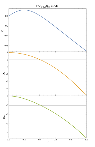
The phase space, matter density parameter, and effective equation of state of the $\beta_{1,1}\beta_{2,1}$ model are presented in fig. 2 for the representative value $B_{11}=1$. The general behavior is similar to the $\beta_{1}$ model in bigravity (see Ref. Könnig et al. (2014a)), with a finite branch over the range $[0,r_{1}^{\text{fix}}]$ and an infinite branch over $[r_{1}^{\text{fix}},\infty]$ with $r_{1}^{\text{fix}}$ being the final value of $r_{1}$ for both branches. The behavior of $\Omega_{\text{m}}$ and $w_{\text{eff}}$ indicates that the infinite branch is not viable as the matter density parameter is always negative and the effective equation of state is always phantom. The finite branch behaves well as there is a matter-dominated past with $w_{\text{eff}}^{\text{init}}=0$, and $w_{\text{eff}}$ evolves towards a de Sitter point with $\Omega_{\text{m}}^{\text{fin}}=0$ and $w_{\text{eff}}^{\text{fin}}=-1$ as in standard cosmology.

Indeed, the $g_{\mu\nu}$ Friedmann eq. 30 can be transformed into the corresponding equation in bigravity using eq. 67,

$$3\mathcal{H}^{2}=\frac{a^{2}\rho_{\text{m}}}{M_{\mathrm{Pl}}^{2}}+3a^{2}(\beta_{1,1}r_{1}+\beta_{2,1}r_{2})=\frac{a^{2}\rho_{\text{m}}}{M_{\mathrm{Pl}}^{2}}+3a^{2}\underbrace{\beta_{1,1}(B_{11}^{2}+1)r_{1}}_{\equiv\beta_{1}r},$$ (72)

where $\beta_{1}$ and $r$ are, respectively, the interaction parameter and ratio of the scale factors in $\beta_{1}$ bigravity (see Ref. Könnig et al. (2014a) for the notation). That means that, at the background level, the $\beta_{1,1}\beta_{2,1}$ model is completely equivalent to the $\beta_{1}$ model of bigravity. We leave it for future work to analyze whether this equivalence still holds at the level of linear perturbations.

IV.1.2 The $\beta_{1,1}\beta_{2,2}$ and $\beta_{1,2}\beta_{2,3}$ models

According to eq. 31, $r_{1}$ in the $\beta_{1,1}\beta_{2,2}$ model is non-dynamical and given by $r_{1}=\frac{1}{3B_{12}}$. Therefore we express everything in terms of $r_{2}$, with the derivative

$$r_{2}^{\prime}=\frac{3-3r_{2}^{2}-B_{12}^{-2}}{2r_{2}}.$$ (73)

We can read off the fixed point as

$$r_{2}^{\text{fix}}=\sqrt{1-\frac{1}{3B_{12}^{2}}}.$$ (74)

Since $r_{2}^{\text{fix}}$ has to be a real number, we have to distinguish between three qualitatively different cases: (a) $B_{12}>1/\sqrt{3}$, (b) $B_{12}=1/\sqrt{3}$, and (c) $B_{12}<1/\sqrt{3}$. For case (a) there is one fixed point, $r_{2}^{\text{fix}}$, and one singular point, $0$, for case (b) there is only one fixed point, $0$, and for case (c) there are no fixed points, but it has one singular point, $0$. The matter density parameter is

$$\Omega_{\text{m}}=1-r_{2}^{2}-\frac{1}{3B_{12}^{2}},$$ (75)

while the effective equation of state is independent of $r_{2}$ and $B_{12}$; it is in fact a constant: $w_{\text{eff}}=-1$ at all times. This is enough to rule the model out as an effective equation of state of $w_{\text{eff}}=-1$ at all times would lead to an accelerated expansion at all times, which clearly contradicts observations. In addition, we can see from eq. 75 that for cases (b) and (c), i.e., for $B_{12}\leq 1/\sqrt{3}$, the matter density parameter is negative, i.e., $\Omega_{\text{m}}\leq 0$, during the entire evolution, which additionally excludes those cases. The $\beta_{1,1}\beta_{2,2}$ model is therefore not viable and we do not present its phase space here.

The $\beta_{1,2}\beta_{2,3}$ model is completely analogous to the model discussed here if we replace $r_{2}$ by $r_{1}$. In this model, $r_{2}$ is non-dynamical and given by $r_{2}=B_{23}^{-1}$. Thus, this model is ruled out as well because of the same arguments as in the $\beta_{1,1}\beta_{2,2}$ model.

IV.1.3 The $\beta_{1,1}\beta_{2,3}$ model

Here, the scale factor ratios $r_{1}$ and $r_{2}$ are related via $r_{2}=\frac{1}{3B_{13}r_{1}}$, which is the simplified form of eq. 31. Plugging this into eq. 35 gives

$$r_{1}^{\prime} =\frac{r_{1}-27B_{13}r_{1}^{3}+81B_{13}^{2}r_{1}^{5}}{1-9B_{13}^{2}r_{1}^{2}-27B_{13}^{2}r_{1}^{4}},$$ (76)

which allows us to find the fixed and singular points

$$r_{1}^{\text{fix}\pm} =\frac{1}{3\sqrt{2}}\sqrt{3\pm B_{13}^{-1}\sqrt{9B_{13}^{2}-4}},$$ (77)

$$r_{1}^{\text{sing}} =\frac{1}{2\sqrt{3}}\sqrt{-3+B_{13}^{-1}\sqrt{3(3B_{13}^{2}+4)}}.$$ (78)

From this we find three cases for the model: (a) $B_{13}>2/3$, (b) $B_{13}=2/3$, and (c) $B_{13}<2/3$. These should be analyzed separately as the qualitative behavior of the phase space is different in each case. For case (a) there are two fixed points and one singular point, while for case (b) there is only one fixed point. Case (c) admits only one singular point, and no fixed point. Before analyzing the three cases one by one, we obtain the simplified form of the matter density parameter and the effective equation of state:

$$\Omega_{\text{m}} =1-3r_{1}^{2}-\frac{1}{27B_{13}^{2}r_{1}^{2}},$$ (79)

$$w_{\text{eff}} =-\Bigl{[}\Bigl{(}1-\frac{1}{27B_{13}^{2}}r_{1}^{-4}\Bigr{)}r_{1}^{\prime}+3r_{1}+\frac{1}{27B_{13}^{2}}r_{1}^{-3}\Bigr{]}r_{1}.$$ (80)

Figure 3: Left panel: Evolution of $r_{1}^{\prime}$, the matter density parameter $\Omega_{\text{m}}$, and the effective equation of state $w_{\text{eff}}$ in terms of $r_{1}$ for the $\beta_{1,1}\beta_{2,3}$ model of star trigravity with $B_{13}=\{2,20\}$. Right panel: Time evolution of $r_{1}$, $\Omega_{\text{m}}$, and $w_{\text{eff}}$ for the finite branch $[r_{1}^{\text{sing}},r_{1}^{\text{fix}+}]$ of the $\beta_{1,1}\beta_{2,3}$ model with $B_{13}=2$, together with the time evolution of $\Omega_{\text{m}}$ and $w_{\text{eff}}$ for standard $\Lambda$CDM cosmology. The right vertical line shows $N=0$, i.e., today, while the left vertical line represents the would-be initial value of $N$ for $B_{13}=2$, i.e., the would-be initial size of the Universe.

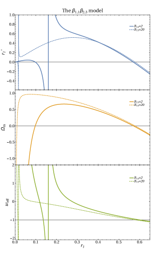
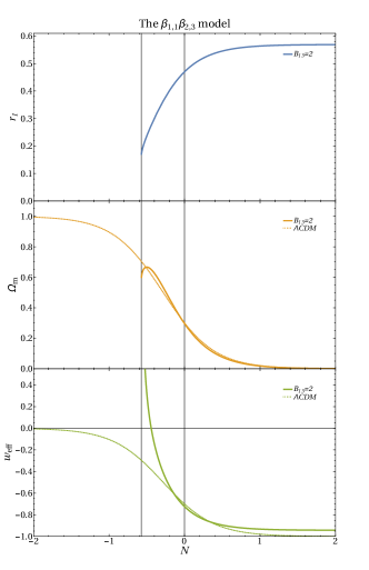
$\bullet$ Case (a): The quantities $r_{1}^{\prime}$, $\Omega_{\text{m}}$, and $w_{\text{eff}}$ as functions of $r_{1}$ are shown in fig. 3 (left panel) for two examples of $B_{13}=2,20$. We can see from the figure that there are four branches in each case. The finite branch $[0,r_{1}^{\text{fix}-}]$ and the infinite branch $[r_{1}^{\text{fix}+},\infty]$ are ruled out because $\Omega_{\text{m}}<0$ on those branches. On the branch $[r_{1}^{\text{fix}-},r_{1}^{\text{sing}}]$, the matter density is positive, $\Omega_{\text{m}}>0$, and decreases with time, but the effective equation of state is phantom during matter domination and is positive when the matter density parameter vanishes. This branch is therefore ruled out.

We are thus left with only the finite branch $[r_{1}^{\text{sing}},r_{1}^{\text{fix}+}]$. The scale factor ratio increases from $r_{1}^{\text{sing}}$, where the matter density parameter takes its initial value

$$\Omega_{\text{m}}^{\text{init}}=2+\frac{8}{9B_{13}^{2}-3B_{13}\sqrt{3(3B_{13}^{2}+4)}}<1,$$ (81)

to the de Sitter point $r_{1}^{\text{fix}+}$ with a vanishing matter density parameter $\Omega_{\text{m}}^{\text{fin}}=0$. $\Omega_{\text{m}}$ first increases to the maximum value

$$\Omega_{\text{m}}^{\text{max}}\equiv 1-\frac{2}{3B_{13}}$$ (82)

at $r_{1}^{\text{max}}=\frac{1}{3\sqrt{B_{13}}}$ and then decreases towards the de Sitter point. At early times, the effective equation of state is singular.

In order to analyze this branch further, we integrate eq. 76 w.r.t $N\equiv\ln a$ to calculate the evolution of the matter density parameter and the effective equation of state. As the initial condition we set $r_{1,0}\equiv r_{1}(N=0)=0.47$ for $B_{13}=2$, in order to achieve a present-time matter density parameter of $\Omega_{\text{m},0}\approx 0.3$ (consistent with observational measurements). The results for $B_{13}=2$ are presented in fig. 3 (right panel) together with the time evolution of $\Omega_{\text{m}}$ and $w_{\text{eff}}$ for $\Lambda$CDM with $\Omega_{\text{m,0}}=0.3$, for comparison.

Since $r_{1}$ starts to evolve from its singular value, there is only a finite number of $e$-foldings in the past. In our $B_{13}=2$ example, the initial number of $e$-foldings is $N_{0}\approx-0.57$. That would imply that the Universe had started to evolve with a finite size $a_{0}=e^{N_{0}}$ such that there would be no big bang. Although we have not presened in the figure, our analysis of the behavior of the model for $B_{13}=20$ compared to $B_{13}=2$ indicates that increasing the value of $B_{13}$ might help to push the singularity back in time and gain larger numbers of $e$-foldings. The maximum value of the matter density parameter will then be closer to $1$. For example, if we choose $B_{13}=700000$, the initial number of $e$-foldings will be $N_{0}\approx-5.3$. For larger values of $B_{13}$ numerical instability leads to problems. However, a value $B_{13}\gg 1$ seems to be unnatural.

$\bullet$ Cases (b) and (c): From eq. 82 we can read off that any value $B_{13}\leq 2/3$ will lead to a negative matter density parameter, $\Omega_{\text{m}}\leq 0$. Thus these cases do not lead to a viable phenomenology. Therefore, we do not present the phase space for these cases.

IV.1.4 The $\beta_{1,2}\beta_{2,2}$ model

Since in this case eq. 31 does not yield a relation between the two scale factor ratios $r_{1}$ and $r_{2}$, and, additionally, eq. 32 is not applicable, the procedure for finding the phase space for the $\beta_{1,2}\beta_{2,2}$ model is rather different. First, we notice that eq. 31 results in $\beta_{1,2}=\beta_{2,2}\equiv\beta$, and therefore, the interaction parameter ratio is fixed to $B_{22}=1$, and there is no free parameter left at the level of the phase space. The Friedmann eqs. 30 and 27 then read

$$3\mathcal{H}^{2}= 3a^{2}\beta(r_{1}^{2}+r_{2}^{2})+a^{2}\frac{\rho_{\text{m}}}{M_{\text{g}}^{2}},$$ (83)

$$3\mathcal{H}^{2}= 3a^{2}\beta.$$ (84)

By subtracting these equations we find

$$\frac{\rho_{\text{m}}}{M_{\text{g}}^{2}}=3\beta(1-r_{1}^{2}-r_{2}^{2}),$$ (85)

which is in agreement with eq. 36. Taking the derivative of eq. 33 with respect to the number of $e$-foldings $N$ yields

$$r_{1}r_{1}^{\prime}+r_{2}r_{2}^{\prime}=\frac{3}{2}(1-r_{1}^{2}-r_{2}^{2}),$$ (86)

after plugging in eqs. 34 and 85. According to eq. 38, the matter density parameter reads

$$\Omega_{\text{m}}=1-r_{1}^{2}-r_{2}^{2}.$$ (87)

Looking at these equations it seems that the phase space for this model is $2$-dimensional, which will make the dynamical analysis more complicated. Let us however try to find a $1$-dimensional phase space for the model, by changing our dynamical variables. We define the variable $r$ as $r^{2}\equiv r_{1}^{2}+r_{2}^{2}$, in terms of which the equations above can be written as

$$3\mathcal{H}^{2}= 3a^{2}\beta r^{2}+a^{2}\frac{\rho_{\text{m}}}{M_{\text{g}}^{2}},$$ (88)

$$r^{\prime}= \frac{3}{2}(r^{-1}-r),$$ (89)

$$\Omega_{\text{m}}= 1-r^{2}.$$ (90)

We can therefore see that the dynamics of the model are completely captured in terms of our new variable $r$, which has a $1$-dimensional phase space, with the fixed and singular points $r^{\text{fix}}=1$ and $r^{\text{sing}}=0$, respectively. What is missing is an expression for the effective equation of state. In order to find it we start with LABEL:{eq:T1-M22-fi-friedmann} and take its derivative with respect to $N$, which yields $\mathcal{H}^{\prime}=a\sqrt{\beta}$ as $a^{\prime}=a$. Plugging this into eq. 40 together with eq. 84 we find a constant effective equation of state, independent of $r$: $w_{\text{eff}}=-1$.

Since the effecive equation of state is constant with $w_{\text{eff}}=-1$ at all times, this model is clearly ruled out. Thus we do not present the phase space of this model.

IV.1.5 The $\beta_{1,3}\beta_{2,3}$ model

In this model, the unique relation between the two scale factor ratios is $r_{2}=B_{33}^{-1}r_{1}$, such that eq. 35 becomes

$$r_{1}^{\prime} =\frac{3r_{1}-(B_{33}^{-2}+1)r_{1}^{3}}{(B_{33}^{-2}+1)r_{1}^{2}-1},$$ (91)

allowing us to read off the fixed and the singular points

$$r_{1}^{\text{fix}} =\frac{\sqrt{3}B_{33}}{\sqrt{B_{33}^{2}+1}},$$ (92)

$$r_{1}^{\text{sing}} =\frac{1}{\sqrt{B_{33}^{-2}+1}}.$$ (93)

We see that there are no cases to be distinguished. The matter density parameter and the effective equation of state are

$$\Omega_{\text{m}} =1-\frac{B_{33}^{-2}+1}{3}r_{1}^{2},$$ (94)

$$w_{\text{eff}} =-\frac{1}{3}(B_{33}^{-2}+1)(r_{1}^{\prime}+r_{1})r_{1}.$$ (95)

Looking at fig. 4, for the parameter choice of $B_{33}=2$ without loss of generality, we can identify three branches. The finite branch $[0,r_{1}^{\text{sing}}]$ is not viable as $\Omega_{\mathrm{m}}$ increases with time and $w_{\text{eff}}$ is always positive, i.e., the branch does not give a late-time acceleration. The infinite branch $[r_{1}^{\text{fix}},\infty]$ is also ruled out as $\Omega_{\text{m}}<0$ always. Finally, on the intermediate finite branch $[r_{1}^{\text{sing}},r_{1}^{\text{fix}}]$, the matter density parameter decreases to its final value $\Omega_{\text{m}}^{\text{fin}}=0$, but its initial value is $\Omega_{\mathrm{m}}^{\text{init}}=2/3$. Since, additionally, the effective equation of state is phantom at all times, this branch is also ruled out.

Figure 4: Evolution of $r_{1}^{\prime}$, the matter density parameter $\Omega_{\text{m}}$, and the effective equation of state $w_{\text{eff}}$ in terms of $r_{1}$ for the $\beta_{1,3}\beta_{2,3}$ model of star trigravity with an interaction parameter ratio of $B_{33}=2$.

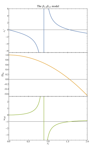
IV.1.6 Summary

We now summarize the phenomenology of the $1+1$-parameter models of star trigravity. This is presented in table 1, where we briefly describe the behavior of $\Omega_{\text{m}}$ and $w_{\text{eff}}$ for different models, their cases and branches. As $\Omega_{\text{m}}<0$ for all infinite branches of $1+1$-parameter star trigravity models, there are no viable such branches, and we therefore do not mention them in the table in order to keep things simple.

A $\checkmark$ in the matter density parameter column means that it decreases from $\Omega_{\text{m}}^{\text{init}}=1$ to $\Omega_{\text{m}}^{\text{fin}}=0$ monotonically, i.e., as in the standard $\Lambda$CDM model. A $\checkmark$ in the effective equation of state column means that $w_{\text{eff}}=0$ in the matter-dominated epoch (at early times) and $w_{\text{eff}}=-1$ at late times, again similarly to $\Lambda$CDM. Otherwise, if $\Omega_{\text{m}}$ and/or $w_{\text{eff}}$ do not behave as in standard cosmology, we briefly describe their behavior, and point out whether/why the phenomenology of the model/branch is new or unviable.

			Viability criterion
Model	Case	Branch	$\Omega_{\text{m}}$	$w_{\text{eff}}$	Phenomenology
$\beta_{1,1}\beta_{2,1}$		Finite	$\checkmark$	$\checkmark$	Standard
$\beta_{1,1}\beta_{2,2}$	$B_{12}>1/\sqrt{3}$	Finite	$\Omega_{\text{m}}^{\text{init}}<1$	Constant $w_{\text{eff}}$: $w_{\text{eff}}=-1$	Unviable
	$B_{12}=1/\sqrt{3}$	Finite	$\Omega_{\text{m}}<0$	Constant $w_{\text{eff}}$: $w_{\text{eff}}=-1$	Unviable
	$B_{12}<1/\sqrt{3}$		$\Omega_{\text{m}}<0$	Constant $w_{\text{eff}}$: $w_{\text{eff}}=-1$	Unviable
$\beta_{1,1}\beta_{2,3}$	$B_{13}>2/3$	$[0,r_{1}^{\text{fix}-}]$	$\Omega_{\text{m}}<0$	$w_{\text{eff}}>0$	Unviable
		$[r_{1}^{\text{fix}-},r_{1}^{\text{sing}}]$	$\Omega_{\text{m}}^{\text{init}}<1$	Phantom at early and positive at late times	Unviable
		$[r_{1}^{\text{sing}},r_{1}^{\text{fix}+}]$	First increases and then decreases to zero	Positive at early times	New
	$B_{13}=2/3$	Finite	$\Omega_{\text{m}}<0$	$w_{\text{eff}}>0$	Unviable
	$B_{13}<2/3$	Finite	$\Omega_{\text{m}}<0$	$w_{\text{eff}}>0$	Unviable
$\beta_{1,2}\beta_{2,2}$		Finite	$\checkmark$	Constant $w_{\text{eff}}$: $w_{\text{eff}}=-1$	Unviable
$\beta_{1,3}\beta_{2,3}$		$[0,r_{1}^{\text{sing}}]$	Increases in time	$w_{\text{eff}}>0$	Unviable
		$[r_{1}^{\text{sing}},r_{1}^{\text{fix}}]$	$\Omega_{\mathrm{m}}^{\mathrm{init}}=2/3$	Phantom at all times	Unviable

Table 1: An overview of the cosmological viability of different $1+1$-parameter models in star trigravity. We consider different branches for different cases in each model. We do not present infinite branches as for all of them $\Omega_{\text{m}}<0$, making the models unviable. The only viable models are the finite branch of the $\beta_{1,1}\beta_{2,1}$ model, with a phenomenology similar to that of the $\beta_{1}$ model of bigravity at the background level, and the intermediate finite branch of the $\beta_{1,1}\beta_{2,3}$ model with a new phenomenology.

The table shows that we are left with only two models that are not ruled out by our analysis. The finite branch of the $\beta_{1,1}\beta_{2,1}$ model behaves exactly like the $\beta_{1}$ model of bigravity at the background level. Therefore we already know that it has a viable background cosmology. A next natural step could then be to study linear perturbations for the model to see if the gradient instabilities, which are present in the finite branch of $\beta_{1}$ bigravity, are absent in the $\beta_{1,1}\beta_{2,1}$ model. The finite branch $[r_{1}^{\text{sing}},r_{1}^{\text{fix}+}]$ of the $\beta_{1,1}\beta_{2,3}$ model behaves differently from any bigravity models, and therefore gives rise to a new phenomenology. Although it seems to be difficult to achieve a viable cosmology with this model, it is not necessarily ruled out. By choosing a very large value for $B_{13}$ one can make this model describe the late-time evolution of the Universe, i.e., after the matter-radiation equality. However, such a large value of $B_{13}$ seems unnatural.

IV.2 Path trigravity

We now repeat the procedure of the previous section for path trigravity. We first simplify eqs. 57 and 58, relating the two scale factor ratios $r_{i}$ by specifying the $\beta_{i,n}$, and rewrite these equations in terms of $B_{mn}$ defined by eq. 64. We then simplify the differential eq. 61 for $r_{1}$ and read off the fixed and singular points. As the final step, we simplify eq. 62 for the matter density parameter $\Omega_{\text{m}}$ and eq. 63 for the effective equation of state $w_{\text{eff}}$. We apply the procedure to all possible $1+1$-parameter models of path trigravity, one by one; these are the nine models $\beta_{1,1}\beta_{2,1}$, $\beta_{1,1}\beta_{2,2}$, $\beta_{1,1}\beta_{2,3}$, $\beta_{1,2}\beta_{2,1}$, $\beta_{1,2}\beta_{2,2}$, $\beta_{1,2}\beta_{2,3}$, $\beta_{1,3}\beta_{2,1}$, $\beta_{1,3}\beta_{2,2}$, and $\beta_{1,3}\beta_{2,3}$.

IV.2.1 The $\beta_{1,1}\beta_{2,1}$ model

For this model, the relations between the two scale factor ratios $r_{1}$ and $r_{2}$, as well as their time derivatives eq. 58, simplify to

$$r_{2}^{\pm}=\frac{\pm\sqrt{12B_{11}^{2}r_{1}^{6}+1}-1}{6B_{11}r_{1}^{3}},\ \ r_{2}^{\prime}=\frac{r_{2}^{2}+2B_{11}r_{1}^{3}r_{2}-6B_{11}r_{1}^{3}r_{2}^{3}}{B_{11}r_{1}^{4}(1+3r_{2}^{2})}r_{1}^{\prime},$$ (96)

where $r_{2}^{\pm}$ are the two roots of eq. 57. The root $r_{2}^{-}$ does not yield consistent results because $\Omega_{\text{m}}>1$ always. Thus, we will focus only on $r_{2}^{+}$ to rewrite $r_{2}$ in terms of $r_{1}$. The differential eq. 61 for $r_{1}$ simplifies to

$$r_{1}^{\prime}=\frac{3r_{1}(1-3r_{1}^{2}+3B_{11}r_{1}^{3}r_{2})(1+3r_{2}^{2})}{1-12B_{11}r_{1}^{3}r_{2}+3r_{1}^{2}(1+3r_{2}^{2})}.$$ (97)

We can read off the fixed points

$$r_{1}^{\text{fix}}=0,\ \ r_{1}^{\text{fix}\pm}=\frac{\sqrt{3\pm\sqrt{9-4B_{11}^{2}}}}{\sqrt{2}B_{11}},$$ (98)

which means that we should distinguish between the qualitatively different cases (a) $B_{11}>3/2$, (b) $B_{11}=3/2$, and (c) $B_{11}<3/2$. The matter density parameter and the effective equation of state are given by

$$\Omega_{\text{m}} =1-\frac{3r_{1}^{2}}{1+3B_{11}r_{1}^{3}r_{2}},$$ (99)

$$w_{\text{eff}} =-\frac{(r_{1}^{\prime}+3r_{1})r_{1}}{1+3B_{11}r_{1}^{3}r_{2}}.$$ (100)

Figure 5: Evolution of $r_{1}^{\prime}$, $\Omega_{\text{m}}$ and $w_{\text{eff}}$ as functions of $r_{1}$ for the $\beta_{1,1}\beta_{2,1}$ model of path trigravity with ratio of the interaction parameters $B_{11}=1.8$ representing case (a).

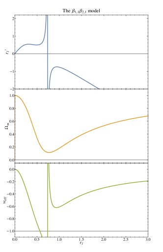
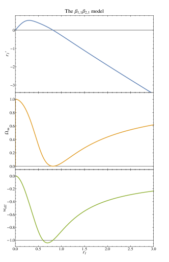
$\bullet$ Case (a): As presented in fig. 5, there is a finite branch, as well as an infinite one, which are separated by a singular point $r_{1}^{\text{sing}}$. Let us first discuss the finite branch. The matter density parameter decreases from $\Omega_{\text{m}}^{\text{init}}=1$ to a finite final value $\Omega_{\text{m}}^{\text{fin}}>0$, i.e., there is no de Sitter point in the infinite future. Such so-called scaling solutions, as mentioned in the beginning of section IV, are the ones with matter and dark energy density parameters approaching constant non-vanishing values in the future. The exact expression for $\Omega_{\text{m}}^{\text{fin}}=\left.\Omega_{\text{m}}\right|_{r_{1}=r_{1}^{\text{sing}}}$ is quite lengthy, but can be found analytically. In fact, the final value of $\Omega_{\text{m}}$ depends on the value of $B_{11}$ such that $\Omega_{\text{m}}^{\text{fin}}$ increases as $B_{11}$ increases. This places an upper bound on the value of $B_{11}$ if we want a certain final value for the matter density parameter. For the case of $\Omega_{\text{m}}^{\text{fin}}\leq 0.3$, this upper limit is $B_{11}\approx 2.8$. Thus, we are left with $B_{11}\in(2/3,2.8)$ in order to have a scaling solution with $\Omega_{\text{m}}^{\text{fin}}\leq 0.3$. The effective equation of state starts from $0$ and then decreases with time, becoming phantom at late times.

Figure 6: Evolution of $r_{1}$, $\Omega_{\text{m}}$, and $w_{\text{eff}}$ as functions of $N=\ln a$ in the $\beta_{1,1}\beta_{2,1}$ model of path trigravity with $B_{11}=1.8$ representing case (a). In order to compare to standard cosmology, the evolution of $\Omega_{\text{m}}$ and $w_{\text{eff}}$ are plotted also for $\Lambda$CDM with $\Omega_{\text{m},0}=0.3$. The left vertical line represents $N=0$ (today). Left panel: Evolution for the finite branch $[0,r_{1}^{\text{sing}}]$, where the right vertical line, at $N=0.28$ (in the future), represents the time at which $r_{1}$ takes its final value $r_{1}^{\text{sing}}$. Right panel: Evolution for the infinite branch $[r_{1}^{\text{sing}},\infty]$, where the right vertical line, at $N=0.57$, represents the time at which $r_{1}$ takes its final value $r_{1}^{\text{sing}}$.

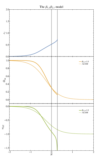
These statements, however, do not rule this model out, and we should therefore analyze the model further as it has a new phenomenology; we do this by integrating the differential eq. 97 numerically for this finite branch with $B_{11}=1.8$. To integrate eq. 97, we choose as the initial condition $r_{1,0}\equiv r_{1}(N=0)=0.52$. This value is chosen such that we obtain a present-time value of the matter density parameter of $\Omega_{\text{m},0}\approx 0.3$. This should be considered only as a representative example; an extensive and careful statistical analysis is needed in order to see whether this model is consistent with cosmological observations. The time evolution of the quantities $r_{1}$, $\Omega_{\text{m}}$, and $w_{\text{eff}}$ are presented in fig. 6 (left panel). For comparison, we have plotted also the time evolution of $\Omega_{\text{m}}$ and $w_{\text{eff}}$ for standard $\Lambda$CDM cosmology. The results show that, at late times, the effective equation of state is negative and with larger absolute values than the ones in $\Lambda$CDM for this path trigravity model. This however may not be a problem, as the average value of $w_{\text{eff}}$ at low redshifts, a quantity that is usually measured from observations, could be similar to the one in $\Lambda$CDM, and therefore, a more detailed statistical analysis is required to test the model observationally. The model however predicts that the evolution continues for only about $0.28$ $e$-foldings in the future. At that time, $r_{1}$ reaches its final value given by $r_{1}^{\text{sing}}$ at which $r_{i}^{\prime}\rightarrow\infty$ for both $i=1,2$. From $w_{\text{eff}}\rightarrow-\infty$ at the singular point we can deduce that $\mathcal{H}^{\prime}\rightarrow\infty$. To summarize, the model approaches a singular point after some finite time, a which the size of the Universe is finite ($\sim e^{0.28}$ times its size today), and the matter density parameter takes a finite value $\Omega_{\text{m}}>0$, but $\mathcal{H}^{\prime}\rightarrow\infty$. This does not rule out the model and one should compare the model’s predictions to observational data.

Let us now turn to the infinite branch. The matter density parameter behaves as in the finite branch with the same finite final value. However, the effective equation of state first decreases, starting with $w_{\text{eff}}^{\text{init}}=0$, during matter domination to a minimum value and then increases at late times towards $+\infty$.

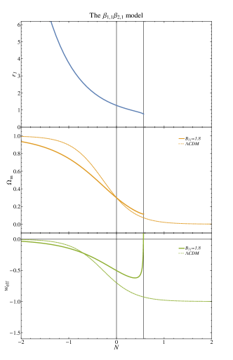
In order to further investigate this branch, we integrate the differential eq. 97. As the initial condition we choose $r_{1,0}=r_{1}(N=0)=1.27$ in order to achieve a present-time value of $\Omega_{\text{m,0}}\approx 0.3$. Again, this should be considered as a representative example. The time evolution of $r_{1}^{\prime}$, $\Omega_{\text{m}}$, and $w_{\text{eff}}$ are presented in the right panel of fig. 6 where we have also included the time evolution of $\Omega_{\text{m}}$ and $w_{\text{eff}}$ for standard $\Lambda$CDM cosmology for comparison. The results show that the effective equation of state is larger than the one in $\Lambda$CDM at late times, but this might not be a problem as explained before. This model predicts that the evolution of the Universe continues only for about $0.57$ $e$-foldings in the future. The scale factor ratio takes its final value $r_{1}^{\text{sing}}$ and the matter density parameter approaches a constant but non-vanishing value $\Omega_{\text{m}}^{\text{fin}}$. While the size of the Universe is finite at this final point ($\sim e^{0.58}$ times its size today), the model predicts a decelerated expansion because $\mathcal{H}^{\prime}\rightarrow-\infty$. This branch is not ruled out by this analysis, and a detailed comparison to observational data is necessary in order to further constrain the model or to finally rule it out.

Figure 7: The $\beta_{1,1}\beta_{2,1}$ model of path trigravity with the ratio of the interaction parameters $B_{11}=1.5$ representing case (b). Left panel: Evolution of $r_{1}^{\prime}$, $\Omega_{\text{m}}$, and $w_{\text{eff}}$ as functions of $r_{1}$. Right panel: Evolution of $r_{1}$, $\Omega_{\text{m}}$, and $w_{\text{eff}}$ as functions of $N\equiv\ln a$ for the finite branch of the model. The vertical line represents $N=0$ (today). In order to compare to standard cosmology, the evolution of $\Omega_{\text{m}}$ and $w_{\text{eff}}$ is plotted also for $\Lambda$CDM with $\Omega_{\text{m},0}=0.3$.

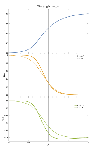
$\bullet$ Case (b): As shown in the left panel of fig. 7, this case admits a finite and an infinite branch separated by the fixed point $r_{1}^{\text{fix}}=\frac{2}{3}\sqrt{\frac{3}{2}}$. In both branches the matter density parameter decreases from $\Omega_{\text{m}}^{\text{init}}=1$ to $\Omega_{\text{m}}^{\text{fin}}=0$ as in standard cosmology. The effective equation of state starts off with $w_{\text{eff}}^{\text{init}}=0$ during matter domination and becomes $w_{\text{eff}}^{\text{fin}}=-1$ at late times, again for both branches. Although the infinite branch has a standard phenomenology, on the finite branch, there is a period at late times when the effective equation of state is phantom, i.e., $w_{\mathrm{eff}}<-1$. This branch has a non-standard phenomenology and needs further analysis in order to check its viability. Therefore, we solve the differential eq. 97 numerically subject to the initial condition $r_{1}(N=0)=0.51$, where $N=0$ corresponds to today, and show the result in the right panel of fig. 7. This initial value has been chosen in such a way that the model gives a present-time matter density parameter of $\Omega_{\text{m},0}\approx 0.3$. This then results in a present-time effective equation of state of $w_{\text{eff},0}\approx-0.88$. Again, as the measured value of $w_{\text{eff}}$ from observations is usually an average over about one $e$-folding, this model could very well be viable, as far as the background cosmology is concerned. The standard $\Lambda$CDM evolution of $\Omega_{\text{m}}$ and $w_{\text{eff}}$ is also plotted for comparison. We can therefore conclude that the model has an interesting new phenomenology, allowing for a phantom equation of state at late times, which cannot be ruled out at this stage and needs further investigation. In order to find out whether the model can successfully describe the late-time evolution of the Universe, one needs to perform a statistical analysis and compare the model to observational data; we leave this for future work.

Figure 8: Left panel: The evolution of $r_{1}^{\prime}$, $\Omega_{\text{m}}$, and $w_{\text{eff}}$ as functions of $r_{1}$ for the $\beta_{1,1}\beta_{2,1}$ model of path trigravity with $B_{11}=1$ representing case (c). Right panel: The same for the $\beta_{1,1}\beta_{2,2}$ model of path trigravity with the interaction parameter ratio of $B_{12}=1$.

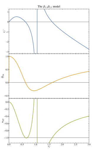
$\bullet$ Case (c): The model admits a finite branch $[0,r_{1}^{\text{fix}-}]$, an infinite branch $[r_{1}^{\text{fix}+},\infty]$, and two intermediate finite branches $[r_{1}^{\text{fix}-},r_{1}^{\text{sing}}]$ and $[r_{1}^{\text{sing}},r_{1}^{\text{fix}+}]$ separated by a singular point $r_{1}^{\text{sing}}$ as can be seen in the left panel of fig. 8. Neither of the intermediate branches is viable as the matter density parameter is negative for the entire evolution. On the finite and infinite branches, $\Omega_{\text{m}}$ and $w_{\text{eff}}$ follow the standard behavior (as for the finite branches of bigravity) such that these branches are viable at the background level.

IV.2.2 The $\beta_{1,1}\beta_{2,2}$ model

This model is described by the following equations:

$$r_{2}^{\pm}=\pm\sqrt{1-\frac{1}{3B_{12}r_{1}^{3}}},\ \ r_{2}^{\prime}=\frac{1-6B_{12}r_{1}^{3}(r_{2}^{2}-1)}{6B_{12}r_{1}^{4}r_{2}}r_{1}^{\prime}.$$ (101)

Here, $r_{2}^{\pm}$ are the two roots of eq. 57; they both lead to the same results. The derivative of $r_{1}$ is given by

$$r_{1}^{\prime} =-3\frac{1-B_{12}r_{1}}{1-2B_{12}r_{1}}r_{1},$$ (102)

from which we can read off two fixed and one singular point:

$$r_{1}^{\text{fix,I}} =0,$$ (103)

$$r_{1}^{\text{fix,II}} =B_{12}^{-1},$$ (104)

$$r_{1}^{\text{sing}} =(2B_{12})^{-1}.$$ (105)

The matter density parameter and the effective equation of state are given by

$$\Omega_{\text{m}} =1-B_{12}^{-1}r_{1},$$ (106)

$$w_{\text{eff}} =-\frac{(r_{1}^{\prime}+3r_{1})r_{1}}{1+3B_{12}r_{1}^{3}r_{2}^{2}}.$$ (107)

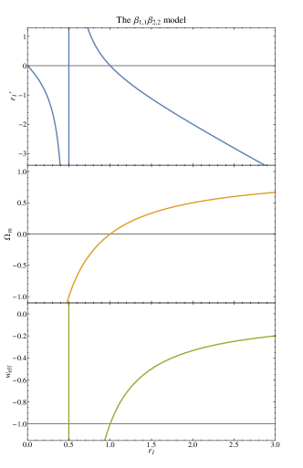
As presented in the right panel of fig. 8 for a representative value of $B_{12}$ (i.e., $B_{12}=1$), there are two finite branches, $[0,r_{1}^{\text{sing}}]$ and $[r_{1}^{\text{sing}},r_{1}^{\text{fix,II}}]$, and an infinite branch $[r_{1}^{\text{fix,II}},\infty]$. Both finite branches are ruled out because $\Omega_{\text{m}}<0$ for the entire evolution of the Universe. The infinite branch however admits a standard phenomenology with $\Omega_{\text{m}}$ evolving from $1$ to $0$ and $w_{\text{eff}}$ evolving from $0$ to $-1$.

IV.2.3 The $\beta_{1,1}\beta_{2,3}$ model

For this model, eq. 57 has three roots:

$$r_{2}^{\text{I}}=\left(\frac{\sqrt{1-4B_{13}^{2}r_{1}^{6}}-1}{2B_{13}r_{1}^{3}}\right)^{\frac{1}{3}}+\left(\frac{\sqrt{1-4B_{13}^{2}r_{1}^{6}}-1}{2B_{13}r_{1}^{3}}\right)^{-\frac{1}{3}},$$ (108)

$$r_{2}^{\text{II}}=-\frac{1-i\sqrt{3}}{2}\left(\frac{\sqrt{1-4B_{13}^{2}r_{1}^{6}}-1}{2B_{13}r_{1}^{3}}\right)^{\frac{1}{3}}-\frac{1+i\sqrt{3}}{2}\left(\frac{\sqrt{1-4B_{13}^{2}r_{1}^{6}}-1}{2B_{13}r_{1}^{3}}\right)^{-\frac{1}{3}},$$ (109)

$$r_{2}^{\text{III}}=-\frac{1+i\sqrt{3}}{2}\left(\frac{\sqrt{1-4B_{13}^{2}r_{1}^{6}}-1}{2B_{13}r_{1}^{3}}\right)^{\frac{1}{3}}-\frac{1-i\sqrt{3}}{2}\left(\frac{\sqrt{1-4B_{13}^{2}r_{1}^{6}}-1}{2B_{13}r_{1}^{3}}\right)^{-\frac{1}{3}}.$$ (110)

The derivatives of the two scale factor ratios are uniquely related via

$$r_{2}^{\prime} =\frac{1-2B_{13}r_{1}^{3}r_{2}(r_{2}^{2}-3)}{3B_{13}r_{1}^{4}(r_{2}^{2}-1)}r_{1}^{\prime},$$ (111)

while the differential eq. 61 simplifies to

$$r_{1}^{\prime}=\frac{3r_{1}(1-r_{2}^{2})(1-3r_{1}^{2}+B_{13}r_{1}^{3}r_{2}^{3})}{1+4B_{13}r_{1}^{3}r_{2}^{3}+3r_{1}^{2}(1-r_{2}^{2})}.$$ (112)

The matter density parameter and the effective equation of state for the model are

$$\Omega_{\text{m}} =1-\frac{3r_{1}^{2}}{1+B_{13}r_{1}^{3}r_{2}^{3}},$$ (113)

$$w_{\text{eff}} =-\frac{(r_{1}^{\prime}+3r_{1})r_{1}}{1+B_{13}r_{1}^{3}r_{2}^{3}}.$$ (114)

Figure 9: Left panel: Evolution of $r_{1}^{\prime}$, $\Omega_{\text{m}}$, and $w_{\text{eff}}$ as functions of $r_{1}$ for the $\beta_{1,1}\beta_{2,3}$ model of path trigravity with the interaction parameter ratios of $B_{13}=2$ (solid lines) representing case (Ia) and $B_{13}=0.5$ (dotted lines) representing case (Ib). Right panel: The same for the $\beta_{1,2}\beta_{2,1}$ model of path trigravity with the interaction parameter ratio of $B_{21}=1$ representing case (a).

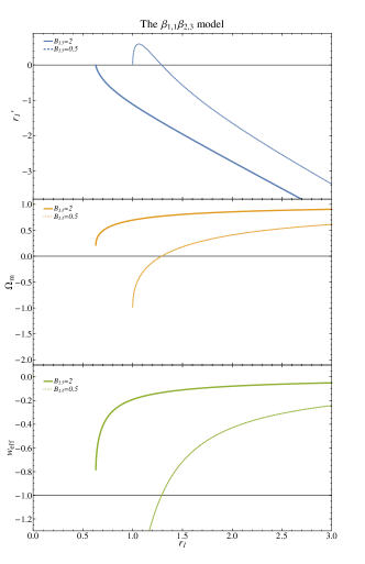
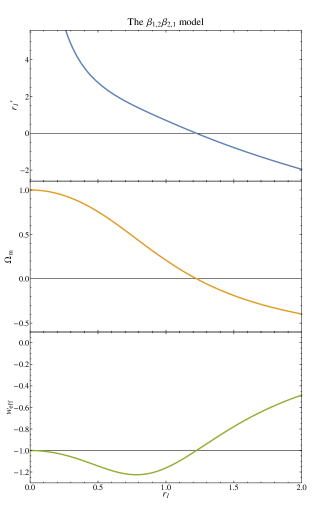
The root $r_{2}^{\text{II}}$ leads to a positive effective equation of state for any value of $B_{13}$ and we conclude that this root does not lead to viable results without presenting the phase space. The root $r_{2}^{\text{III}}$ produces a negative matter density parameter, $\Omega_{\text{m}}<0$, for any value of $B_{13}$ and thus the phenomenology is not viable. Only the root $r_{2}^{\text{I}}$ needs a more detailed analysis and we therefore focus on eq. 108 relating $r_{2}$ and $r_{1}$. We have to distinguish the two cases (Ia) $B_{13}\gtrsim 1.12$ with one fixed point $r_{1}^{\text{fix,I}}$ and (Ib) $B_{13}\lesssim 1.12$ with two fixed points $r_{1}^{\text{fix,I}}$ and $r_{1}^{\text{fix,II}}$. We do not present the analytical expressions of the fixed points here as they are quite lengthy. Using eq. 108, $r_{1}^{\prime}$ is real only in the interval $[r_{1}^{\mathrm{fix,I}},\infty]$.

$\bullet$ Case (Ia): As presented in fig. 9 (left panel) for the representative value of $B_{13}=2$, there is only an infinite branch $[r_{1}^{\text{fix,I}},\infty]$. For $r_{1}<r_{1}^{\text{fix,I}}$, $r_{1}^{\prime}$ takes complex values and thus the model’s phase space is limited to the interval $[r_{1}^{\text{fix,I}},\infty]$. Although the matter density parameter and the effective equation of state initially behave as in the standard phenomenology, i.e., $\Omega_{\text{m}}^{\text{init}}=1$ and $w_{\text{eff}}^{\text{init}}=0$, they approach values $\Omega_{\text{m}}^{\text{fin}}>0$ and $w_{\text{eff}}^{\text{fin}}>-1$ in the future. This is again a scaling solution.

A more careful investigation of the model, however, reveals some subtleties at and close to $r_{1}^{\text{fix,I}}$ which must be taken into account when interpreting its cosmological implications. If the point is really a fixed point, then the matter density parameter will become a constant in the future and since the continuity eq. 34 implies $\rho_{\text{m}}\propto a^{-3}$, the Hubble parameter must evolve as $\mathcal{H}^{2}\propto a^{-3}$. This implies $w_{\text{eff}}=0$, which contradicts eq. 114 as can be seen in fig. 9 (left panel) where $w_{\text{eff}}$ is negative in the future. The reason for this contradiction can however be understood by looking at how $r_{1}$, $r_{2}$, and their derivatives evolve with time. At the point given by $r_{1}^{\prime}=0$ we have $r_{2}=1$, such that we divide by $0$ in eq. 111, and therefore eq. 58 is not valid at that point. In fact we have $r_{2}^{\prime}\neq 0$ as can be found by taking the derivative of eq. 108. In addition, we find that $\mathrm{d}r_{2}/\mathrm{d}r_{1}$ and $\mathrm{d}r_{2}^{\prime}/\mathrm{d}r_{1}$ are both singular at this point. This all means that the point with $r_{1}^{\prime}=0$ is not really a fixed point of the system because $r_{2}^{\prime}\neq 0$. Since the derivatives of some quantities are singular at this point, we call it a singular fixed point. With the analysis developed and used in this paper it is not possible to make predictions for singular fixed points, and their analysis is beyond the scope of this work. We therefore leave a careful treatment of models with singular fixed points for future work.

Note however that our analysis does not rule this case out, if the singular fixed point can be pushed to a time far in the future. The question of what happens to the Universe when it approaches this singularity is an interesting one that needs to be explored. Situations with such singular fixed points occur in path trigravity $1+1$-parameter models only when $\beta_{2,3}\neq 0$, as can be seen by looking at the denominator of eq. 58. In that case, the denominator will have a term $\propto(1-r_{2}^{2})$. Whenever we get to a point with $r_{2}^{2}=1$ our analysis does not work because eq. 58 is not valid. One possible way to deal with such a singularity is to not use eqs. 57 and 58 to rewrite $r_{2}$ in terms of $r_{1}$, but to treat $r_{1}$ and $r_{2}$ as two independent dynamical variables subject to the Friedmann eqs. 50, 53 and 54, and then to analyze the $2$-dimensional phase space numerically. Since this requires a type of analysis that is different from our approach in this paper, we leave it for future work.

$\bullet$ Case (Ib): As presented in fig. 9 (left panel) for the representative value of $B_{13}=0.5$ there is one finite and one infinite branch. The infinite branch $[r_{1}^{\text{fix,II}},\infty]$ produces the standard phenomenology with $\Omega_{\text{m}}$ evolving from $1$ to $0$ and $w_{\text{eff}}$ evolving from $0$ to $-1$. The finite branch $[r_{1}^{\text{fix,I}},r_{1}^{\text{fix,II}}]$ is not viable because $\Omega_{\text{m}}<0$ always. For $r_{1}<r_{1}^{\text{fix,I}}$, $r_{1}^{\prime}$ takes complex values and thus the phase space is limited to the interval $[r_{1}^{\text{fix,I}},\infty]$.

IV.2.4 The $\beta_{1,2}\beta_{2,1}$ model

The phase space for this model is described by

$$r_{1}^{\prime}=\frac{3(1+3r_{2}^{2})(1-r_{1}^{2}+B_{21}r_{1}^{2}r_{2})}{2r_{1}(1-2B_{21}r_{2}+3r_{2}^{2})},$$ (115)

with $r_{2}$ and its time derivative given in terms of $r_{1}$ and $r_{1}^{\prime}$ as

$$r_{2}^{\pm}=\frac{\pm\sqrt{9+12B_{21}^{2}r_{1}^{4}}-3}{6B_{21}r_{1}^{2}},\ \ r_{2}^{\prime}=\frac{2r_{2}-6r_{2}^{3}}{r_{1}+3r_{1}r_{2}^{2}}r_{1}^{\prime},$$ (116)

where $r_{2}^{\pm}$ are again the two roots of eq. 57. The root $r_{2}^{-}$ leads to sulutions with $\Omega_{\text{m}}>1$ and $w_{\text{eff}}>0$ always, and we therefore focus only on $r_{2}^{+}$ when rewriting $r_{2}$ in terms of $r_{1}$ in the following expressions. The model possesses one fixed point which is given by

$$r_{1}^{\text{fix}}=\sqrt{\frac{3}{3-B_{21}^{2}}}.$$ (117)

We have to distinguish the three cases (a) $B_{21}<\sqrt{3}$, (b) $B_{21}=\sqrt{3}$, and (c) $B_{21}>\sqrt{3}$. The matter density parameter and the effective equation of state are

$$\Omega_{\text{m}} =1-\frac{r_{1}^{2}}{1+B_{21}r_{1}^{2}r_{2}},$$ (118)

$$w_{\text{eff}} =-\frac{(2r_{1}^{\prime}+3r_{1})r_{1}}{3+3B_{21}r_{1}^{2}r_{2}}.$$ (119)

Figure 10: Evolution of $r_{1}^{\prime}$, $\Omega_{\text{m}}$, and $w_{\text{eff}}$ as functions of $r_{1}$ for the $\beta_{1,2}\beta_{2,1}$ model of path trigravity with the interaction parameter ratios of $B_{21}=\sqrt{3}$ (left panel) representing case (b) and $B_{21}=2$ (right panel) representing case (c).

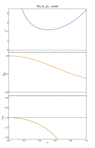
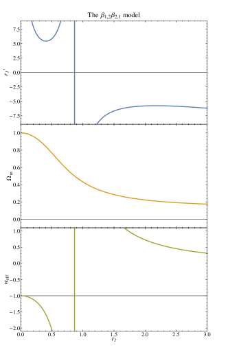
$\bullet$ Case (a): As presented in fig. 9 (right panel) for the representative value $B_{21}=1$, the model contains a finite and an infinite branch. The infinite branch $[r_{1}^{\text{fix}},\infty]$ is not viable as $\Omega_{\text{m}}<0$ always. On the finite branch $[0,r_{1}^{\text{fix}}]$, the scale factor ratio $r_{1}$ increases starting at the singular point $r_{1}=0$. The matter density parameter decreases from $1$ to $0$ as in standard cosmology, but the effective equation of state is phantom for the entire evolution of the Universe, even during matter domination. We therefore conclude that this case is not viable.

$\bullet$ Case (b): As presented in fig. 10 (left panel) for the value $B_{21}=\sqrt{3}$, the model contains only one finite branch $[0,\infty]$. The scale factor ratio $r_{1}$ increases starting at the singular point $r_{1}=0$. The matter density parameter decreases from $1$ to $0$ as in standard cosmology, but the effective equation of state is phantom at all times. Thus, this case does not have a viable cosmology.

$\bullet$ Case (c): As presented in fig. 10 (right panel) for the representative value $B_{21}=2$, the model contains a finite and an infinite branch, separated by a singular point. While the effective equation of state is phantom on the finite branch during the entire evolution of the Universe, it is positive on the infinite branch. Therefore, this case does not have a viable phenomenology.

IV.2.5 The $\beta_{1,2}\beta_{2,2}$ model

The relation between $r_{2}$ and $r_{1}$ is given by

$$r_{2}^{\pm}=\pm\sqrt{1-\frac{1}{B_{22}r_{1}^{2}}},\ \ r_{2}^{\prime}=\frac{1-r_{2}^{2}}{r_{1}r_{2}}r_{1}^{\prime},$$ (120)

where both roots $r_{2}^{\pm}$ of eq. 57 lead to the same results. The evolution equation of $r_{1}$ is

$$r_{1}^{\prime} =-\frac{3}{2}r_{1}.$$ (121)

The only fixed point of the model can be read off as $r_{1}^{\text{fix}}=0$ and therefore there are no different cases in this model that we need to distinguish between. The matter density parameter simplifies to $\Omega_{\text{m}}=1-B_{22}^{-1}$ and thus is a constant that does not depend on $r_{1}$. The effective equation of state is also a constant: $w_{\text{eff}}=0$.

Since the matter density parameter and the effective equation of state are both constants and do not depend on $r_{1}$, we can immediately conclude that this model is not viable. We therefore do not present its phase space.

IV.2.6 The $\beta_{1,2}\beta_{2,3}$ model

The derivative of the scale factor ratio, eq. 61, simplifies to

$$r_{1}^{\prime}=3\frac{(1-r_{2}^{2})(3-3r_{1}^{2}+B_{23}r_{1}^{2}r_{2}^{3})}{2r_{1}(3-3r_{2}^{2}+2B_{23}r_{2}^{3})}.$$ (122)

For this model, eq. 57 leads to three different possible relations between $r_{1}$ and $r_{2}$ that are not redundant at the level of the Friedmann equations:

$$r_{2}^{\text{I}} =\left(\frac{\sqrt{9-4B_{23}^{2}r_{1}^{4}}-3}{2B_{23}r_{1}^{2}}\right)^{-1/3}+\left(\frac{\sqrt{9-4B_{23}^{2}r_{1}^{4}}-3}{2B_{23}r_{1}^{2}}\right)^{1/3},$$ (123)

$$r_{2}^{\text{II}} =-\frac{1+i\sqrt{3}}{2}\left(\frac{\sqrt{9-4B_{23}^{2}r_{1}^{4}}-3}{2B_{23}r_{1}^{2}}\right)^{-1/3}-\frac{1-i\sqrt{3}}{2}\left(\frac{\sqrt{9-4B_{23}^{2}r_{1}^{4}}-3}{2B_{23}r_{1}^{2}}\right)^{1/3},$$ (124)

$$r_{2}^{\text{III}} =-\frac{1-i\sqrt{3}}{2}\left(\frac{\sqrt{9-4B_{23}^{2}r_{1}^{4}}-3}{2B_{23}r_{1}^{2}}\right)^{-1/3}-\frac{1+i\sqrt{3}}{2}\left(\frac{\sqrt{9-4B_{23}^{2}r_{1}^{4}}-3}{2B_{23}r_{1}^{2}}\right)^{1/3}.$$ (125)

The quantity $r_{2}$ and its derivative are uniquely related as

$$r_{2}^{\prime} =\frac{2r_{2}(3-r_{2}^{2})}{3r_{1}(r_{2}^{2}-1)}.$$ (126)

The matter density parameter and the effective equation of motion are given by

$$\Omega_{\text{m}} =1-\frac{3r_{1}^{2}}{3+B_{23}r_{1}^{2}r_{2}^{3}},$$ (127)

$$w_{\text{eff}} =-\frac{(2r_{1}^{\prime}+3r_{1})r_{1}}{3+B_{23}r_{1}^{2}r_{2}^{3}}.$$ (128)

Figure 11: Evolution of $r_{1}^{\prime}$, $\Omega_{\text{m}}$, and $w_{\text{eff}}$ as functions of $r_{1}$ for the $\beta_{1,2}\beta_{2,3}$ model of path trigravity with the interaction parameter ratios of $B_{23}=2$ (solid lines) representing case (Ia) and $B_{23}=0.7$ (dotted lines) representing case (Ib).

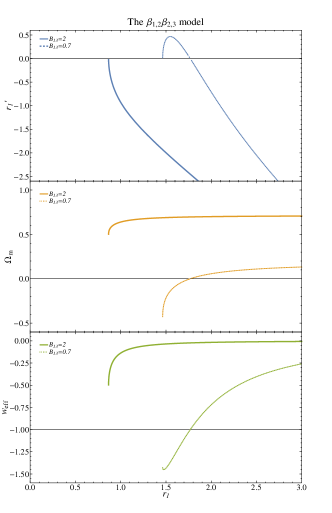
The root $r_{2}^{\text{II}}$ leads to $\Omega_{\text{m}}>1$ for any values of $B_{23}$ and $r_{1}$, and has therefore no viable phenomenology. If we choose $r_{2}^{\text{III}}$ to relate the two scale factor ratios, the matter density is negative always, $\Omega_{\text{m}}<0$, leading to an unviable phenomenology. These two cases are ruled and and we do not present their phase spaces. We therefore focus only on $r_{2}^{\text{I}}$ relating $r_{2}$ and $r_{1}$. We should distinguish between two different cases: (Ia) $B_{23}\gtrsim 0.9$ with one fixed point $r_{1}^{\mathrm{fix,I}}$, and (Ib) $B_{23}\lesssim 0.9$ with two fixed points $r_{1}^{\mathrm{fix,I}}$ and $r_{2}^{\mathrm{fix,II}}$. The analytic expressions of the fixed points are quite lengthy and we do not present them here. Moreover, for values $B_{23}\leq 0.5$, $r_{1}^{\prime}$ takes complex values and we are therefore limited to values of the interaction parameter ratio of $B_{23}>0.5$ in case (Ib); using eq. 123, $r_{1}^{\prime}$ is real only in the interval $[0,r_{1}^{\mathrm{fix,I}}]$.

$\bullet$ Case (Ia): As presented in fig. 11 for the representative value of $B_{23}=2$, there is only an infinite branch $[r_{1}^{\text{fix,I}},\infty]$. For $r_{1}<r_{1}^{\text{fix,I}}$, $r_{1}^{\prime}$ takes complex values and thus the model’s phase space is limited to the interval $[r_{1}^{\text{fix,I}},\infty]$. This model yields a scaling solution with $\Omega_{\text{m}}^{\text{fin}}>0$ and $w_{\text{eff}}^{\text{fin}}>-1$. This case is another example for a singular fixed point, discussed in section IV.2.3. Since we cannot apply the method used in this paper to such cases, we leave a detailed analysis of this singular fixed point for future work.

$\bullet$ Case (Ib): As presented in fig. 11 for the representative value of $B_{23}=0.7$, there is one finite and one infinite branch. The infinite branch $[r_{1}^{\text{fix,II}},\infty]$ produces the standard phenomenology with $\Omega_{\text{m}}$ evolving from $1$ to $0$ and $w_{\text{eff}}$ evolving from $0$ to $-1$. The finite branch $[r_{1}^{\text{fix,I}},r_{1}^{\text{fix,II}}]$ is not viable because $\Omega_{\text{m}}<0$ and $w_{\text{eff}}<-1$ always. For $r_{1}<r_{1}^{\text{fix,I}}$, $r_{1}^{\prime}$ takes complex values and thus the phase space is limited to the interval $[r_{1}^{\text{fix,I}},\infty]$.

IV.2.7 The $\beta_{1,3}\beta_{2,1}$ model

For this model, the derivative of the scale factor ratio, eq. 61, simplifies to

$$r_{1}^{\prime}=\frac{r_{1}(3-r_{1}^{2}+3B_{31}r_{1}r_{2})(1+3r_{2}^{2})}{-1-4B_{31}r_{1}r_{2}+r_{1}^{2}(1+3r_{2}^{2})},$$ (129)

where $r_{2}$ and its derivative are given by

$$r_{2}^{\pm} =\frac{\pm\sqrt{9+6r_{1}+r_{1}^{2}+12B_{31}r_{1}^{2}}-3-r_{1}}{6B_{31}r_{1}},$$ (130)

$$r_{2}^{\prime} =-\frac{(3r_{2}-2B_{31}r_{1}+6B_{31}r_{1}r_{2}^{2})r_{2}}{B_{31}r_{1}^{2}(1+3r_{2}^{2})}r_{1}^{\prime},$$ (131)

with $r_{2}^{\pm}$ being the two roots of eq. 57. The root $r_{2}^{-}$ does not lead to consistent results because $\Omega_{\text{m}}<0$ always, and we will therefore use only $r_{2}^{+}$ in our studies of the cosmological solutions for this model. The model has two fixed points, $r_{1}^{\text{fix,I}}=0$ and $r_{1}^{\text{fix,II}}$, which exist for all values of $B_{31}$. The analytic expression for $r_{1}^{\text{fix,II}}$ is quite lengthy and we do not present it here. The matter density parameter and the effective equation of state are

$$\Omega_{\text{m}} =1-\frac{r_{1}^{2}}{3+3B_{31}r_{1}r_{2}},$$ (132)

$$w_{\text{eff}} =-\frac{(r_{1}^{\prime}+r_{1})r_{1}}{3+3B_{31}r_{1}r_{2}}.$$ (133)

Figure 12: Evolution of $r_{1}^{\prime}$, $\Omega_{\text{m}}$, and $w_{\text{eff}}$ as functions of $r_{1}$ for the $\beta_{1,3}\beta_{2,1}$ model of path trigravity with an interaction parameter ratio of $B_{31}=1$.

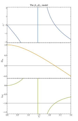
As shown in fig. 12 for the representative value $B_{31}=1$, there are three branches in this model. The infinite branch $[r_{1}^{\text{fix,II}},\infty]$ is not viable as $\Omega_{\text{m}}<0$, always. The finite branch $[0,r_{1}^{\text{sing}}]$ is not viable either as $\Omega_{\text{m}}$ increases with time. In addition, $w_{\text{eff}}$ is always positive on this branch, which does not allow an accelerating universe. On the finite branch $[r_{1}^{\text{sing}},r_{1}^{\text{fix,II}}]$, the matter density parameter starts off with $\Omega_{\text{m}}^{\text{init}}<1$, decreases in time, and vanishes in the infinite future, but the effective equation of state is always phantom, rendering the model unviable.

IV.2.8 The $\beta_{1,3}\beta_{2,2}$ model

The phase space of this model is described by

$$r_{1}^{\prime} =3r_{1}^{-1}-r_{1}+3B_{32}r_{2}^{2},$$ (134)

where the two scale factor ratios $r_{1}$ and $r_{2}$, and their time derivatives, are related via

$$r_{2}^{\pm}=\pm\sqrt{1-\frac{3+r_{1}}{3B_{32}r_{1}}},\ \ r_{2}^{\prime}=-\frac{1-2B_{32}r_{1}(1-r_{2}^{2})}{2B_{32}r_{1}^{2}r_{2}}r_{1}^{\prime}.$$ (135)

Both roots $r_{2}^{\pm}$ of eq. 57 lead to the same results. The model has the fixed point

$$r_{1}^{\text{fix}}=3B_{32}-1,$$ (136)

such that we have to distinguish the cases $B_{32}>1/3$ with two fixed points $r_{1}^{\text{fix}}$ and $0$, and $B_{32}\leq 1/3$ with only one fixed point $0$. The matter density parameter and the effective equation of state are

$$\Omega_{\text{m}} =1-\frac{r_{1}^{2}}{3+3B_{32}r_{1}r_{2}^{2}},$$ (137)

$$w_{\text{eff}} =-\frac{r_{1}^{\prime}+r_{1}}{3+3B_{32}r_{1}r_{2}^{2}}.$$ (138)

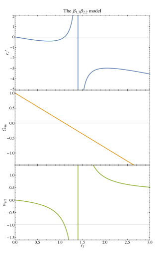
We first rewrite $r_{2}$ in the expression of $\Omega_{\text{m}}$ using eq. 135 to get $\Omega_{\text{m}}=1-\frac{r_{1}}{3B_{32}-1}$. We can infer that the values of the interaction parameter ratios $B_{32}=1/3$ and $B_{32}<1/3$ do not lead to viable phenomenologies. For $B_{32}=1/3$ the matter density parameter is infinite and for $B_{32}<1/3$, it will be larger than $1$. We therefore restrict our discussion to $B_{32}>1/3$. The same procedure for the effective equation of state yields $w_{\text{eff}}=\frac{(1-B_{32})r_{1}}{(1-3B_{32})(2B_{32}-r_{1})}$. The value $B_{32}=1/3$ results in an infinite effective equation of state. Additionally, the value $B_{32}=1$ is special because it leads to a constant effective equation of state $w_{\text{eff}}=0$. Since we can already infer that $B_{32}\leq 1/3$ and $B_{32}=1$ do not yield viable phenomenologies, we do not present the corresponding phase spaces here. We are left with two cases that need further investigation: (a) $B_{32}>1$ and (b) $1/3<B_{32}<1$.

Figure 13: Evolution of $r_{1}^{\prime}$, $\Omega_{\text{m}}$, and $w_{\text{eff}}$ as functions of $r_{1}$ for the $\beta_{1,3}\beta_{2,2}$ model of path trigravity with an interaction parameter ratio of $B_{32}=2$ (left panel) representing case (a) and $B_{32}=0.7$ (right panel) representing case (b).

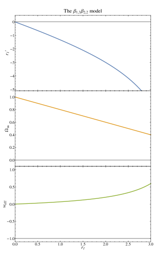
$\bullet$ Case (a): As fig. 13 (left panel) shows for the representative value of $B_{32}=2$, the model has only an infinite branch $[0,\infty]$. The branch is not viable as $\Omega_{\text{m}}$ increases in time and $w_{\text{eff}}$ is positive during the entire evolution of the Universe.

$\bullet$ Case (b): As fig. 13 (right panel) shows for the representative value of $B_{32}=0.7$, the model has two finite and an infinite branch. The finite branch $[0,r_{1}^{\text{fix}}]$ is not viable as $\Omega_{\text{m}}$ and $w_{\text{eff}}$ increase in time. The finite branch $[r_{1}^{\text{fix}},r_{1}^{\text{sing}}]$ and the infinite branch $[r_{1}^{\text{sing}},\infty]$ are both unviable because the matter density parameter is always negative. Therefore, this case does not have a viable cosmology.

IV.2.9 The $\beta_{1,3}\beta_{2,3}$ model

For this model, the derivative of the scale factor ratio, eq. 61, simplifies to

$$r_{1}^{\prime}=\frac{3r_{1}(1-r_{2}^{2})(3-r_{1}^{2}+B_{33}r_{1}r_{2}^{3})}{-3+4r_{1}r_{2}^{3}+3r_{1}^{2}-3r_{1}^{2}r_{2}^{2}}.$$ (139)

There are three different solutions to eq. 57, given by

$$r_{2}^{\text{I}}= \left(\frac{\sqrt{9+6r_{1}+r_{1}^{2}-4B_{33}^{2}r_{1}^{2}}-3-r1}{2B_{33}r_{1}}\right)^{\frac{1}{3}}+\left(\frac{\sqrt{9+6r_{1}+r_{1}^{2}-4B_{33}^{2}r_{1}^{2}}-3-r1}{2B_{33}r_{1}}\right)^{-\frac{1}{3}},$$ (140)

$$r_{2}^{\text{II}}= -\frac{1-i\sqrt{3}}{2}\left(\frac{\sqrt{9+6r_{1}+r_{1}^{2}-4B_{33}^{2}r_{1}^{2}}-3-r1}{2B_{33}r_{1}}\right)^{\frac{1}{3}}$$

$$-\frac{1+i\sqrt{3}}{2}\left(\frac{\sqrt{9+6r_{1}+r_{1}^{2}-4B_{33}^{2}r_{1}^{2}}-3-r1}{2B_{33}r_{1}}\right)^{-\frac{1}{3}},$$ (141)

$$r_{2}^{\text{III}}= -\frac{1+i\sqrt{3}}{2}\left(\frac{\sqrt{9+6r_{1}+r_{1}^{2}-4B_{33}^{2}r_{1}^{2}}-3-r1}{2B_{33}r_{1}}\right)^{\frac{1}{3}}$$

$$-\frac{1-i\sqrt{3}}{2}\left(\frac{\sqrt{9+6r_{1}+r_{1}^{2}-4B_{33}^{2}r_{1}^{2}}-3-r1}{2B_{33}r_{1}}\right)^{-\frac{1}{3}}.$$ (142)

The derivatives are uniquely related via

$$r_{2}^{\prime} =\frac{3+2B_{33}r_{1}r_{2}(3-r_{2}^{2})}{3B_{33}r_{1}^{2}(r_{2}^{2}-1)}r_{1}^{\prime}.$$ (143)

The matter density parameter and the effective equation of state are given by

$$\Omega_{\text{m}} =1-\frac{r_{1}^{2}}{3+B_{33}r_{1}r_{2}^{3}},$$ (144)

$$w_{\text{eff}} =-\frac{(r_{1}^{\prime}+r_{1})r_{1}}{3+B_{33}r_{1}r_{2}^{3}}.$$ (145)

Let us first focus on the roots $r_{2}^{\text{II}}$ and $r_{2}^{\text{III}}$ to relate the two scale factor ratios. While the root $r_{2}^{\text{II}}$ leads to a matter density parameter with $\Omega_{\text{m}}>1$ always, the root $r_{2}^{\text{III}}$ leads to a phantom equation of state with $w_{\text{eff}}<-1$ always, for any values of $B_{33}$ and $r_{1}$. We thus conclude the phenomenology of this model is not viable, if we choose $r_{2}^{\text{II}}$ or $r_{2}^{\text{III}}$ to relate the scale factor ratios.

Let us now turn to the root $r_{2}^{\text{I}}$ in order to relate $r_{2}$ and $r_{1}$. The phase space of this model is quite complex and there exist numerous cases we have to distinguish, but our analysis shows that none of the cases and branches lead to a viable phenomenology as we discuss now without presenting the corresponding phase spaces. For values $B_{33}\lesssim 1.08$ the matter density parameter will be negative at all times, i.e., $\Omega_{\text{m}}\lesssim 0$. In the interval $1.08\lesssim B_{33}\lesssim 1.13$ there is an intermediate finite branch where the matter density parameter starts at $0$, takes a maximum value of $\lesssim 0.13$ and decreases to $0$ again, i.e., there is no matter-dominated era. The other branches have $\Omega_{\text{m}}<0$. For values $B_{33}\gtrsim 1.13$, the matter density parameter is either negative or increasing in time. In addition, the phase space contains a singular fixed point that requires further investigation. To summarize, this model does not have a viable phenomenology.

IV.2.10 Summary

We now summarize the phenomenology of the $1+1$-parameter models of path trigravity. We give an overview of our results in table 2, where we briefly describe the behavior of $\Omega_{\text{m}}$ and $w_{\text{eff}}$ for different models, their cases and branches.

A $\checkmark$ in the matter density parameter column means that $\Omega_{\text{m}}$ starts off with an initial value $\Omega_{\text{m}}^{\text{init}}=1$ and decreases monotonically with time to the final value $\Omega_{\text{m}}^{\text{fin}}=0$, i.e., as in standard $\Lambda$CDM cosmology. A $\checkmark$ in the effective equation of state column means that $w_{\text{eff}}$ starts off with the initial value $w_{\text{eff}}^{\text{init}}=0$ at early times (matter-dominated epoch) and decreases to the final value $w_{\text{eff}}^{\text{fin}}=-1$ at late times, again as in $\Lambda$CDM. Otherwise, if $\Omega_{\text{m}}$ and/or $w_{\text{eff}}$ do not behave as in standard cosmology, we briefly describe their behavior, and point out whether/why the phenomenology of the model/branch is new or unviable.

As summarized in the table, we are left with four viable models:

• The $\beta_{1,1}\beta_{2,1}$-model infinite branches for the cases $B_{11}<3/2$ and $B_{11}=3/2$, as well as the finite branch of the case $B_{11}<3/2$, have fulfilled our viability criteria and have standard phenomenologies. The case $B_{11}=3/2$ has a viable finite branch with a phantom effective equation of state at late times and thus leads to a new phenomenology. Note that in the case $B_{11}=3/2$ the ratio of the interaction parameters is not a free parameter, and is fixed. In the case $B_{11}>3/2$ we find a finite and an infinite branch, both giving rise to new phenomenology. The final value of the matter density parameter is larger than $0$, such that in both branches the model does not approach a de Sitter point in the infinite future, resulting in the so-called scaling solutions. However, the effective equation of state will be singular at late times for both branches, but the initial conditions and $B_{11}$ can be chosen in such a way that the present time value of $w_{\text{eff}}$ is still consistent with observations. Additionally, this case predicts a singular point in the (near) future. One needs to systematically perform a statistical analysis and compare the model’s predictions to data in order to be able to either finally rule this model out or make it a distinguishable alternative to $\Lambda$CDM.

• The $\beta_{1,1}\beta_{2,2}$ model has an infinite branch with a standard phenomenology for any value of $B_{12}$.

• The $\beta_{1,1}\beta_{2,3}$ model has two cases depending on the value of $B_{13}$. For the case $B_{13}\lesssim 1.12$, the model has an infinite branch with standard phenomenology. For values $B_{13}\gtrsim 1.12$ the phase space contains a singular fixed point. With the analysis performed in this paper it is not possible to make predictions about what will happen at such singular fixed points and thus we cannot rule out this model. In order to analyze the model further, one can for example treat both $r_{1}$ and $r_{2}$ as dynamical variables subject to the Friedmann equations and then analyze the full $2$-dimensional phase space.

• For the $\beta_{1,2}\beta_{2,3}$ model, we need to distinguish between two cases depending on the value of $B_{23}$. For $B_{23}\lesssim 0.9$ the phase space contains an infinite branch with standard phenomenology. In the case $B_{23}\gtrsim 0.9$ the phase space contains a singular fixed point. In order to be able to rule out this case, one needs to perform a different analysis than the one performed in this paper.

We have therefore found a number of models that produce the standard phenomenology. That does not mean, however, that the phenomenologies of these models are completely indistinguishable from $\Lambda$CDM. In order to find out whether these models are able to explain the late-time accelerated expansion of the Universe, one needs to perform a statistical analysis, comparing the model’s predictions to observations. Of course, the same needs to be done for the models with new phenomenology.

			Viability criterion
Model	Case	Branch	$\Omega_{\text{m}}$	$w_{\text{eff}}$	Phenomenology
$\beta_{1,1}\beta_{2,1}$	$B_{11}>3/2$	Finite	$\Omega_{\text{m}}^{\text{fin}}>0$	$w_{\text{eff}}^{\text{fin}}\rightarrow-\infty$	New
		Infinite	$\Omega_{\text{m}}^{\text{fin}}>0$	$w_{\text{eff}}^{\text{fin}}\rightarrow\infty$	New
	$B_{11}=3/2$	Finite	$\checkmark$	$w_{\text{eff}}^{\text{late}}<-1$	New
		Infinite	$\checkmark$	$\checkmark$	Standard
	$B_{11}<3/2$	Finite	$\checkmark$	$\checkmark$	Standard
		$[r_{1}^{\text{fix}-},r_{1}^{\text{sing}}]$	$\Omega_{\text{m}}<0$	$w_{\text{eff}}^{\text{init}}\rightarrow\infty$	Unviable
		$[r_{1}^{\text{sing}},r_{1}^{\text{fix}+}]$	$\Omega_{\text{m}}<0$	Phantom	Unviable
		Infinite	$\checkmark$	$\checkmark$	Standard
$\beta_{1,1}\beta_{2,2}$		$[0,r_{1}^{\text{sing}}]$	$\Omega_{\text{m}}<0$	$w_{\text{eff}}>0$	Unviable
		$[r_{1}^{\text{sing}},r_{1}^{\text{fix}}]$	$\Omega_{\text{m}}<0$	Phantom	Unviable
		Infinite	$\checkmark$	$\checkmark$	Standard
$\beta_{1,1}\beta_{2,3}$	$B_{13}\gtrsim 1.12$	Infinite	$\Omega_{\text{m}}^{\text{fin}}>0$	$w_{\text{eff}}^{\text{fin}}>-1$	New
	$B_{13}\lesssim 1.12$	Finite	$\Omega_{\text{m}}<0$	Phantom	Unviable
		Infinite	$\checkmark$	$\checkmark$	Standard
$\beta_{1,2}\beta_{2,1}$	$B_{21}<\sqrt{3}$	Finite	$\checkmark$	Phantom	Unviable
		Infinite	$\Omega_{\text{m}}<0$	$\checkmark$	Unviable
	$B_{21}=\sqrt{3}$	Finite	$\checkmark$	Phantom	Unviable
	$B_{21}>\sqrt{3}$	Finite	$\Omega_{\text{m}}^{\text{fin}}>0$	Phantom	Unviable
		Infinite	$\Omega_{\text{m}}^{\text{init}}<1$, increasing	$w_{\text{eff}}>0$	Unviable
$\beta_{1,2}\beta_{2,2}$		Finite	Constant	Constant	Unviable
$\beta_{1,2}\beta_{2,3}$	$B_{23}\gtrsim 0.9$	Infinite	$\Omega_{\text{m}}^{\text{fin}}>0$	$w_{\text{eff}}^{\text{fin}}>-1$	New
	$B_{23}\lesssim 0.9$	Finite	$\Omega_{\text{m}}<0$	Phantom	Unviable
		Ininite	$\checkmark$	$\checkmark$	Standard
$\beta_{1,3}\beta_{2,1}$		$[0,r_{1}^{\text{sing}}]$	Increasing	$w_{\text{eff}}>0$	Unviable
		$[r_{1}^{\text{sing}},r_{1}^{\text{fix}}]$	$\Omega_{\text{m}}^{\text{init}}<1$	Phantom	Unviable
		Infinite	$\Omega_{\text{m}}<0$	$\checkmark$	Unviable
$\beta_{1,3}\beta_{2,2}$	$B_{32}>1$	Infinite	Increasing	$w_{\text{eff}}>0$	Unviable
	$1/3<B_{32}<1$	$[0,r_{1}^{\text{sing}}]$	Increasing	Increasing	Unviable
		$[r_{1}^{\text{sing}},r_{1}^{\text{fix}}]$	$\Omega_{\text{m}}<0$	Phantom	Unviable
		Infinite	$\Omega_{\text{m}}<0$	$w_{\text{eff}}>0$	Unviable
	$B_{32}=1$			Constant: $w_{\text{eff}}=0$	Unviable
	$B_{32}\leq 1/3$		$\Omega_{\text{m}}>1$ or $\Omega_{\text{m}}=\infty$		Unviable
$\beta_{1,3}\beta_{2,3}$					Unviable

Table 2: An overview of the cosmological viability of different $1+1$-parameter models in path trigravity. We consider different branches for different cases in each model.

V Novel phenomenology

Let us now take a closer look at the results of our analysis summarized in tables 1 and 2. We have identified in total one class of models in star trigravity and three in path trigravity which a) are not immediately ruled out by observations, and b) possess some new phenomenology (as defined in section IV) as far as the background expansion is concerned. These are the $\beta_{1,1}\beta_{2,3}$ star model in one particular branch (what we called intermediate finite branch), as well as the path models $\beta_{1,1}\beta_{2,1}$ with $B_{11}\geq 1.5$, $\beta_{1,1}\beta_{2,3}$ with $B_{13}\gtrsim 1.12$, and $\beta_{1,2}\beta_{2,3}$ with $B_{23}\gtrsim 0.9$.

The first case, i.e., the $\beta_{1,1}\beta_{2,3}$ model of star trigravity, has a matter density parameter $\Omega_{\text{m}}$ that begins with a finite value in the past at $r_{1}=r_{1}^{\text{sing}}$ and ends up in a de Sitter state with $r_{1}=r_{1}^{\text{fix+}}$ and $\Omega_{\text{m}}=0,$ passing through a maximum value. At the same time the effective equation of state $w_{\text{eff}}$ decreases monotonically from infinity to $-1$. By adjusting the value of $B_{13}$ one can obtain a phenomenology that resembles $\Lambda$CDM, moving the singularity far into the past. Therefore, although phenomenologically new, this evolution is actually viable only in the limit in which the model is indistinguishable from $\Lambda$CDM.

The $\beta_{1,1}\beta_{2,1}$ model of path trigravity has two cases giving rise to new phenomenology. For $B_{11}>1.5$ the phase space of the model contains one finite and one infinite branch, separated by a singular point. The past evolution is similar to the standard one on both branches with $\Omega_{\text{m}}^{\text{init}}=1$ and $w_{\text{eff}}^{\text{init}}=0$. Both branches contain a singularity that can be moved to the future. One can adjust the initial conditions and $B_{11}$ so as to get $\Omega_{\text{m},0}\approx 0.3$ and $w_{\text{eff},0}\approx-0.9$ at present time, although rapidly varying with time. The evolution is therefore not standard and might be better constrained, or finally ruled out, by a full comparison with observational data. The other case with $B_{11}=1.5$ is particularly interesting because now the evolution on the finite branch has no singularities and no obvious problems. The ratio of the interaction parameters is not a free parameter in this case, i.e., the model has only one free parameter as in $\Lambda$CDM (either $\beta_{1,1}$ is a free parameter and $\beta_{2,1}$ is fixed or the other way around). This model predicts an effective equation of state smaller than $-1$, i.e., of phantom type, at late times. The asymptotic value is $w_{\text{eff}}^{\text{fin}}=-1$. Initial conditions can be adjusted so as to have $w_{\text{eff}}\approx-0.9$ today. It is possible to have a viable cosmology with a phantom crossing, i.e., evolution of $w_{\text{eff}}$ from above to below $-1$, contrary to the bimetric case where viable models never cross $w_{\mathrm{eff}}=-1$ Könnig et al. (2014a). Again a careful comparison with observations can rule out or confirm the validity of this case.

The path models $\beta_{1,1}\beta_{2,3}$ with $B_{13}\gtrsim 1.12$ and $\beta_{1,2}\beta_{2,3}$ with $B_{23}\gtrsim 0.9$ have similar non-standard phenomenologies. The past evolution is standard for both models with $\Omega_{\text{m}}^{\text{init}}=1$ and $w_{\text{eff}}^{\text{init}}=0$, but the models evolve towards singular fixed points at which $\Omega_{\text{m}}>0$ and $w_{\text{eff}}>-1$. This would identify these solutions as scaling solutions. However, the singular fixed points are not real fixed points at which the evolution stops. In order to predict how the models will evolve when approaching the singular fixed points it might be necessary to analyze their $2$-dimensional phase space.

VI Conclusions and outlook

One of our goals in studying multimetric gravity is to find non-trivial, consistent, simple, and viable alternatives to $\Lambda$CDM. Such cosmologies should be clearly distinguishable from $\Lambda$CDM, be free of ghosts and other instabilities, and possess a small number of free parameters. They should also avoid obvious inconsistencies with observation which can arise in these theories, such as singularities in the observable past, absence of late-time acceleration, and the nonexistence of a matter era. This goal has not yet been reached with theories of massive and bimetric gravity. This failure has prompted us to investigate in detail the cosmology of trimetric gravity in search of alternatives to $\Lambda$CDM. In particular, we explored in some detail all possible forms of trimetric gravity with two free interaction parameters (one for each pair of interacting metrics) and no cosmological constants—the minimal non-trivial models in this framework. We have shown that the phase space of these models in most cases is simple and $1$-dimensional, i.e., the equations for $r_{i}^{\prime}(r)$ depend only on the ratio of the two interaction parameters. For each model, we discussed analytically and numerically the cosmic evolution and determined whether it was compatible with the current understanding of our Universe.

Our main result is that, in addition to many unviable cases, there are a number of models in which the evolution is compatible with observations at the background level, although most are practically indistinguishable from $\Lambda$CDM. In fact, perhaps surprisingly, we find only three cases that appear to be promising alternatives to standard cosmology, all of which have the “path” configuration of interactions in which the two additional metrics couple to the physical spacetime metric but not to each other. The first viable model is that in which only the couplings $\beta_{1,1}$ and $\beta_{2,1}$ are switched on; in particular, if the ratio of the coupling constants is $1.5$, such that the model has only one free parameter, just like $\Lambda$CDM, we find a non-trivial evolution without obvious problems. This case is interesting also because it crosses the phantom divide $w_{\mathrm{eff}}=-1$, contrary to what happens in bimetric models. We have additionally found two cases with scaling solutions, i.e., solutions which do not asymptote to de Sitter at late times. These models contain singular fixed points in the future with possibly interesting implications for cosmology. It is necessary to perform a more detailed ($2$-dimensional) phase-space analysis near the singular points in order to understand how these solutions would evolve when passing through the fixed points.

All the viable trimetric models that we have found in this work, with either new or standard phenomenology, deserve a more detailed treatment in terms of both comparison to observational data and analysis of perturbations. Naturally, the question of whether these models contain instabilities of any kind is of particular importance, as even models with standard phenomenologies at the background level, i.e., the ones that behave similarly to $\Lambda$CDM or bigravity models, may very well behave differently at the perturbative level. In particular, bimetric models with viable backgrounds have been shown to contain instabilities at the level of linear perturbations. With the extra freedom afforded by trimetric gravity, we are optimistic about finding viable and stable alternatives to the standard cosmology within the framework of massive, multimetric theories of gravity. All these questions will be explored in future work.