Disordered XYZ Spin Chain Simulations using the
Spectrum Bifurcation Renormalization Group

Abstract

We study the disordered XYZ spin chain using the recently developed Spectrum Bifurcation Renormalization Group (SBRG) You et al. (2015) numerical method. With strong disorder, the phase diagram consists of three many body localized (MBL) spin glass phases. We argue that, with sufficiently strong disorder, these spin glass phases are separated by marginally many-body localized (MBL) critical lines. We examine the critical lines of this model by measuring the entanglement entropy and Edwards-Anderson spin glass order parameter, and find that the critical lines are characterized by an effective central charge $c^{\prime}=\ln 2$. Our data also suggests continuously varying critical exponents along the critical lines. We also demonstrate how long-range mutual information introduced in Ref. Jian et al. (2015) can distinguish these phases.

I Introduction

Quantum phase transitions Sachdev (2011) were previously discussed as transitions between ground states of quantum many-body systems at zero temperature. The conventional wisdom is that highly excited states of a many-body system at finite energy density are typically self-thermalized following the eigenstate thermalization hypothesis (ETH) Deutsch (1991); Srednicki (1994); Rigol et al. (2008). However, later it was realized that many-body localized (MBL) systems Gornyi et al. (2005); Basko et al. (2006); Oganesyan and Huse (2007); Žnidarič et al. (2008); Imbrie (2014); Nandkishore and Huse (2015) – typically systems with quenched disorder – can evade thermalization and exhibit robust quantum coherence and non-ergodic dynamics even at finite energy density. The phenomenon of many-body localization (MBL) enables quantum phase transitions to occur at a finite energy density between different MBL quantum phases Refael and Altman (2013); Huse et al. (2013); Pekker et al. (2014); Chandran et al. (2014); Vasseur et al. (2015a); Slagle et al. (2015). The corresponding quantum critical points are marginally localized Nandkishore and Potter (2014) and are thus known as marginal MBL states (or quantum critical glasses) Vasseur et al. (2015b). Similar to MBL states, marginal MBL states are also non-ergodic, and can be specified by an extensive number of quasi-local integrals of motion (LIOM) Chandran et al. (2015); Kim et al. (2014); Ros et al. (2015). Unlike the typical MBL states, the marginal MBL states exhibit critical behaviors, including the logarithmic scaling of entanglement entropy (in 1D) and the power-law decay of disorder-averaged correlation functions and mutual information.

In this work, we will study the marginal MBL states in a 1D XYZ spin model using the spectrum bifurcation renormalization group (SBRG) numerical method introduced in Ref. You et al. (2015). SBRG is another version of the excited-state real space renormalization group (RSRG-X) Vosk and Altman (2013); Pekker et al. (2014); Refael and Altman (2013); Vasseur et al. (2015a), which is specifically designed for the class of MBL models that has a bifurcating spectrum branching structure at each renormalization group (RG) step. The idea of SBRG is similar to RSRG-X, which targets the full many-body spectrum rather than just the ground state. Given a many-body Hamiltonian $H$ with strong disorder, at each RG step, the leading energy scale term (the strongest local term) $H_{0}$ in the Hamiltonian $H$ is first selected, and the whole Hamiltonian $H$ is rotated to the block diagonal basis of $H_{0}$. The block off-diagonal terms, which resonate between different $H_{0}$ eigen sectors, are treated as perturbations and are reduced to effective terms within the diagonal block via second order perturbation. The RG procedure gradually block diagonalizes the many-body Hamiltonian until it is fully diagonalized. The resulting effective Hamiltonian $H_{\text{eff}}$ can be viewed as the RG fixed point Hamiltonian for the MBL system Serbyn et al. (2013a, b); Chandran et al. (2015); Huse et al. (2014); Kim et al. (2014), which encodes the full many-body spectrum. The RG transformations can be collected and combined into a unitary quantum circuit $U_{\text{RG}}$ (Fig. 11, 12), which encodes the matrix product state (MPS) approximations for all eigenstates. Various physical properties of the MBL (and marginal MBL) system can be calculated based on the data of $H_{\text{eff}}$ and $U_{\text{RG}}$ generated by SBRG. Unlike RSRG-X, SBRG does not explicitly choose a specific eigen sector at each RG step. Instead, the spectrum branching is encoded implicitly in the flow of the Hamiltonian, such that the entire spectrum is targeted during each RG flow.

There has been a long history of using the real space renormalization group (RSRG) method to study disordered spin chains.Dasgupta and Ma (1980); Bhatt and Lee (1982); Fisher (1992, 1994, 1995) RSRG was originally proposed as a ground state targeting approach, and has been applied to the random Heisenberg,Dasgupta and Ma (1980) transverse field Ising,Fisher (1992, 1995) XY and XXZ Fisher (1994) spin chains. It was found that ground states of (clean) quantum critical spin chains (e.g. Ising, XX or Heisenberg) could be unstable to random exchange couplings and flow to the infinite randomness (strong disorder) fixed-point. Whether the critical phenomena of the infinite randomness fixed-point persists at finite energy density is further discussed in the context of MBL using RSRG-X and other methods Pekker et al. (2014); Vasseur et al. (2015a); Refael and Altman (2013); Vasseur et al. (2015c). The current understanding is that the strong disorder criticality could persist to finite energy density as marginal MBL states in quantum Ising chains. Pekker et al. (2014) But for (planar) XXZ and Heisenberg chains, the marginal MBL state is unstable towards thermalization or spontaneous symmetry breaking Vasseur et al. (2015a, c), due to the extensive number of local degeneracies dictated by the symmetry group. Take the random XXZ chain for example, the symmetry group $U(1)\rtimes\mathbb{Z}_{2}$ is a product of the spin-Z conservation and the spin-flipping $\mathbb{Z}_{2}$ symmetry. Following the argument given in Ref. Potter et al. (2016), the symmetric marginal MBL state, if possible, should be characterized by a set of quasi-LIOM, which form irreducible representations of the $U(1)\rtimes\mathbb{Z}_{2}$ symmetry group. However, the $U(1)\rtimes\mathbb{Z}_{2}$ symmetry enforces a local degeneracy between states of opposite spin-Z for every quasi-LIOM. As a result, the finite energy density eigenstates in the many-body spectrum are all exponentially degenerate. Because the extensive degeneracy is unstable to quantum fluctuations, the eigenstates must either localize to symmetry breaking spin glass states or thermalize, both of which destroy the quantum criticality.

So to explore marginal MBL phases in 1D spin systems, we must sufficiently break the symmetry to remove all local degeneracies. This motivates us to look at the XYZ spin chain, with independently random XX, YY and ZZ couplings on each bond. The symmetry is broken down to $\mathbb{Z}_{2}^{2}$, such that local degeneracies are completely removed (because $\mathbb{Z}_{2}^{2}$ has no irreducible representations beyond the one-dimensional representations). Therefore, marginal MBL states of the XYZ spin chain can be stable at finite energy density against thermalization and spontaneous symmetry breaking as long as the disorder is strong enough. Due to the discrete $\mathbb{Z}_{2}^{2}$ symmetry, at each RG step there is only one unique leading energy scale term that bifurcates the spectrum. This is precisely the type of model that SBRG was designed to target.

Apart from the above symmetry considerations, strong disorder is another key ingredient to keep the marginal MBL states from thermalizing. We introduce the standard deviation of the logarithmic scale of the coupling strengths

$$\Gamma=\mathrm{std}(\ln|J|)$$ (1)

(where $J$ appears as coefficients in the Hamiltonian, e.g. Eq. (2)) to compare the strength of three often used disorder distributions: uniform, Gaussian, and the power-law distribution which will be used in this work. Physically, $\Gamma$ describes how much different couplings are separated in their energy scales. Well separbated energy scales in the large $\Gamma$ limit suppress the resonance between energy levels, and hence hinders thermalization. Our finite-size exact diagonalization (ED) study (Appendix D) indicates that $\Gamma\simeq 1$ is not sufficient to stabilize the marginal MBL phases in the XYZ model against thermalization. Therefore, instead of drawing the coupling strengths from uniform distributions ($\Gamma=1$) or Gaussian distributions ($\Gamma\approx 1.1$), we need to take power-law distributions (Appendix C.1) whose $\Gamma$ can be tuned all the way to infinity. We will typically take $\Gamma=4$ as the initial distribution in our calculation. SBRG is well-suited to study such strong disorder spin systems, as the SBRG algorithm is asymptotically accurate in the large $\Gamma$ limit.

In the following, we will first introduce the model and present the phase diagram. Then we focus on a high symmetry line in the phase diagram, and investigate the MBL spin glass phase and marginal MBL critical phase in detail. In particular, we calculate the entanglement entropy, Edwards-Anderson correlator and long-range mutual information. We found that the marginal MBL critical line is characterized by an effective central charge $c^{\prime}=\ln 2$. Our data also suggest continuously varying exponents along the critical line.

II XYZ Spin Chain Model

We study the XYZ spin chain with large disorder and periodic boundary conditions. The Hamiltonian is given by

$$H=\sum_{i=1}^{L}\sum_{\mu=x,y,z}J_{i,\mu}\;\sigma_{i}^{\mu}\sigma_{i+1}^{\mu}.$$ (2)

$\sigma_{i}^{\mu}$ with $\mu=1,2,3$ are Pauli matrix operators on lattice site $i$ of a 1d chain of length $L$. The couplings $J_{i,\mu}\in[0,J_{\mu}]$ are randomly drawn from a power-law distribution

$$\mathrm{PDF}(J_{i,\mu})=\frac{1}{\Gamma J_{i,\mu}}\left(\frac{J_{i,\mu}}{J_{\mu}}\right)^{1/\Gamma},$$ (3)

where $0<\Gamma<\infty$ (see Eq. (1)) controls the disorder strength (for details see Appendix C.1). Equivalently, $J_{i,\mu}^{1/\Gamma}\in[0,J_{\mu}^{1/\Gamma}]$ is uniformly distributed. For later convenience, we define

$$\tilde{J}_{\mu}\equiv J_{\mu}^{1/\Gamma},$$ (4)

and take $\tilde{J}_{\mu}=\tilde{J}_{x},\tilde{J}_{y},\tilde{J}_{z}$ as our primary tuning parameters (see Appendix C.2 for an explanation). We will be interested in the entire energy spectrum of this model, as opposed to just the low energy states.

Beside the exact global symmetry $\mathbb{Z}_{2}^{2}$, the model also has some statistical symmetries, which are valid only in the statistical sense over the ensemble of the disordered Hamiltonians. When $J_{x}=J_{y}$ (and similarly for $J_{y}=J_{z}$ and $J_{z}=J_{x}$), the distribution of Hamiltonians $H$ has a $\mathbb{Z}_{2}$ symmetry which swaps $J_{i,x}\leftrightarrow J_{i,y}$. When $J_{x}=J_{y}=J_{z}$, the distribution of Hamiltonians has an $S_{3}$ permutation symmetry which permutes $J_{i,x}\leftrightarrow J_{i,y}\leftrightarrow J_{i,z}$. For any $J_{\mu}$, the distribution of Hamiltonians also has translation symmetry. Imposing these statistical symmetries can be used to easily fine tune the XYZ model to its critical phases.

In the existing literature, the RSRG-X approach Pekker et al. (2014); Vasseur et al. (2015a); Refael and Altman (2013); Vasseur et al. (2015c) has been successfully applied to analyze various marginal MBL phases in disordered spin systems. However, it is challenging to apply the traditional closed-form RSRG-X analysis to the XYZ model, even near the free fermion soluble points (such as $J_{x}=J_{y}$ and $J_{z}\to 0$). At the free fermion soluble point, the spin system can be mapped to two independent Majorana chains with uncorrelated randomness, which allows the standard bond decimation RG scheme to be applied independently on each chain. However, once the fermion interactions ($J_{z}$ terms) are introduced to the system, the two Majorana chains are coupled together as a ladder lattice. The independent bond decimation on both chains will quickly distort the ladder lattice and generate complicated configurations of multi-fermion interactions, which can not be tracked in closed-form. Therefore, we turn to the numerical approach of SBRG, which can keep track of all orders of multi-fermion interactions generated under the RG flow.

In the following, we will study the XYZ model by applying SBRG. We will show results for $\Gamma=4$ initial randomness, for which SBRG agrees well with exact diagonalization on small latices (data not shown in this paper), and our approximations appear to be safe (see Appendix B.1 and D, and Sec. III.2). We will also limit our system sizes to $L\leq 256$ because our current implementation of SBRG does not produce accurate results for larger system sizes on the critical lines of the XYZ model.

III Phase Diagram

Figure 1: Ternary plot of the disorder and energy averaged entanglement entropy $S_{\text{E}}$ [bit] ($\equiv S_{\text{E}}/\ln 2$) (Eq. (6)) of a subsystem of length $L/2$ (top) and Edwards-Anderson correlator (Eq. (9)) (bottom) vs coupling constants ($0<\tilde{J}_{x,y,z}<1$) for the XYZ spin chain of length $L=256$. We use this plot to sketch the phase diagram. When $\tilde{J}_{z}>\max(\tilde{J}_{x},\tilde{J}_{y})$, the system is in a $\mathbb{Z}_{2}$ spin glass state. When $\tilde{J}_{z}<\tilde{J}_{x}=\tilde{J}_{y}$, the system is in a marginal MBL phase. (The other phases are given by permutations of $x,y,z$.) The white dots correspond to the points in the phase diagram that are shown in Fig. 4, 5, 7.

III.1 Spin Glass Phases

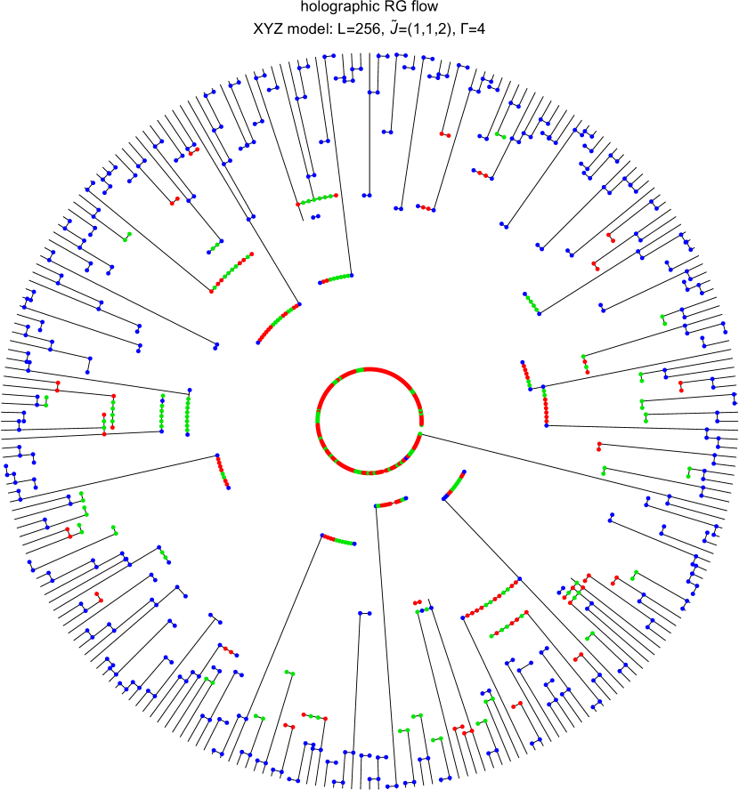
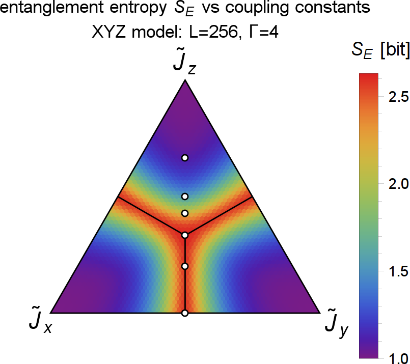
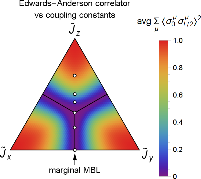
With large disorder and at finite energy density, there are three spin glass phases (Fig. 1). We find that if $\tilde{J}_{z}$ is the largest coupling constant (i.e. $\tilde{J}_{z}>\tilde{J}_{x}$ and $\tilde{J}_{z}>\tilde{J}_{y}$), then the system is in an MBL spin glass phase where the correlator $\sigma_{i}^{z}\sigma_{j}^{z}$ shows long range glassy behavior. That is, $\sigma_{i}^{z}\sigma_{j}^{z}$ develops a finite overlap with products of the local integrals of motion (LIOM) $\tau^{z}$s of the MBL phase (see Eq. (12) in Appendix A), and is thus roughly conserved. This finite overlap results in an Edwards-Anderson correlator that asymptotes to a nonzero constant at large distance, which we take to be the primary signature of a spin glass phase.

III.2 Critical Phases

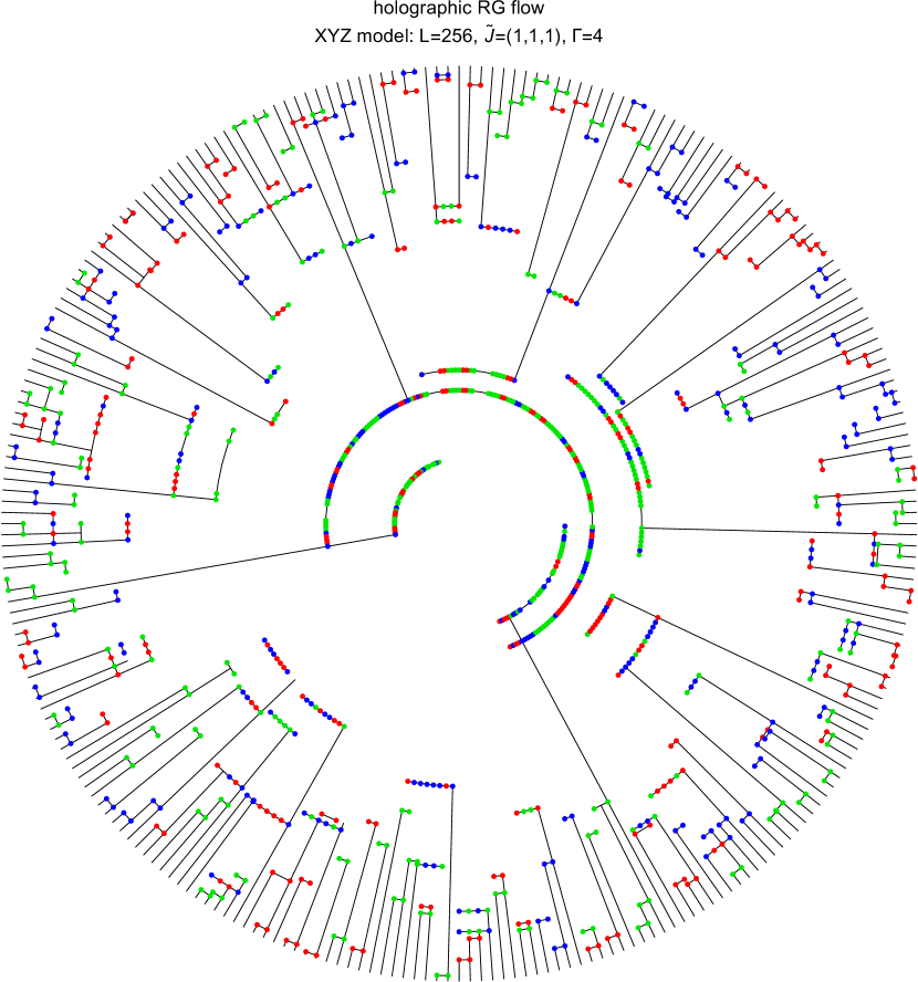
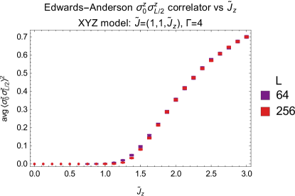
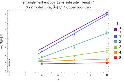
With sufficiently strong disorder, the spin glass phases appear to be separated by a critical lines (e.g. $\tilde{J}_{z}\leq\tilde{J}_{x}=\tilde{J}_{y}$) consisting of marginal MBL phases, which is evidenced by the fact that the entanglement entropy diverges logarithmically (Fig. 4) in this phase. In Fig. 2 we provide evidence that the critical ($\tilde{J}_{z}\leq\tilde{J}_{x}=\tilde{J}_{y}$) to spin glass ($\tilde{J}_{z}>\tilde{J}_{x}=\tilde{J}_{y}$) phase transition is continuous and occurs exactly at $J_{x}=J_{y}=J_{z}$ by showing evidence that the long-range spin glass Edwards-Anderson correlator is zero when $\tilde{J}_{z}\leq\tilde{J}_{x}=\tilde{J}_{y}$ and increases continuously for $\tilde{J}_{z}>\tilde{J}_{x}=\tilde{J}_{y}$. An example of how the LIOM look in this phase is shown in Fig. 11.

Figure 2: Disorder and energy averaged Edwards-Anderson correlator (Eq. (9)) at separation $x=L/2$ vs $\tilde{J}_{z}$ for different system sizes $L$ in the XYZ spin chain with $\tilde{J}_{x}=\tilde{J}_{y}=1$. In the critical phase, the Edwards-Anderson correlator decays algebraically to zero; while in the spin glass phase, the Edwards-Anderson correlator asymptotes to a constant. Furthermore, as one tunes $\tilde{J}_{z}$ from the critical phase to the spin glass phase, the Edwards-Anderson correlator becomes nonzero continuously at $\tilde{J}_{z}=1$, indicating that this marks the location of a continuous phase transition. (error bar details: foo )

Marginal MBL vs Thermal

With sufficiently large disorder, SBRG depicts the critical phase as marginally MBL as SBRG finds a logarithmically diverging entanglement entropy in this phase. However, SBRG is not capable of describing thermalization, and so one should worry that resonance effects may thermalize the critical phase. Indeed, the instability of marginal MBL phase to thermalization has been demonstrated in other 1D spin models. Vasseur et al. (2015a, c) Thus, it is crucial to check the approximations made by SBRG, in order to verify that an exact RG does not flow toward thermalization. In Appendix D we do a brief exact diagonalization study to check that with strong disorder, the system is not thermal. Below, we will study the evidence against thermalization by using SBRG.

The core approximation made by SBRG is the validity of the second order perturbation theory used by each RG step. This and other approximations are explained in detail and accounted for in Appendix B.1. However, even though these approximations are controlled by strong disorder, one could still worry that errors may build up during the RG flow and cause SBRG to incorrectly depict the critical phase as a marginal MBL phase, even if the critical phase is actually thermal.

At intermediate RG steps, a cluster of $n$ “LIOM” could resonate and become thermalized by an off-diagonal term that mixes (i.e. anticommutes with) them if the energy of the off-diagonal term $\varepsilon_{\text{mix}}$ is larger than the smallest energy difference $\Delta E$ of the $n$ “LIOM”: i.e. if $\varepsilon_{\text{mix}}>\Delta E$. The verified assumptions Eq. (14) and 15 imply that this rarely occurs for small $n$. However, one might worry that large clusters of $n$ “LIOM” could be thermalized by rare off-diagonal terms Gopalakrishnan et al. (2015). But a cluster of $n$ LIOM will describe $2^{n}$ states, and thus typically have a smallest energy level spacing equal to $\Delta E\sim 2^{-n}$ (because our model has a small symmetry, there is no symmetry protected degeneracy in this cluster); while below we argue that off-diagonal terms at intermediate RG steps will have energies of order $\varepsilon_{\text{mix}}\lesssim e^{-\Gamma n}$, which is much smaller than $\Delta E\sim 2^{-n}$ for large disorder $\Gamma$. Thus, $\varepsilon_{\text{mix}}\ll\Delta E$ and so it seems unlikely that enough clusters of $n$ “LIOM” could resonate to thermalize the system.

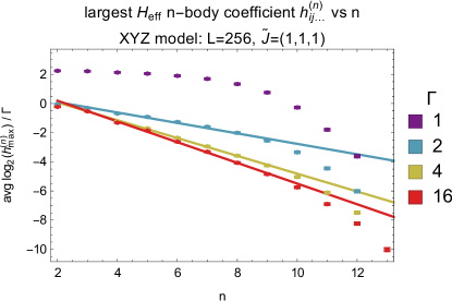
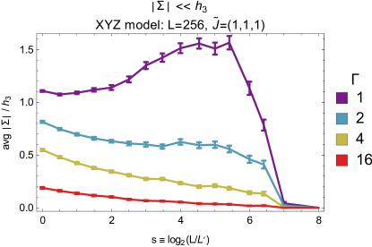
To show that $\varepsilon_{\text{mix}}\lesssim e^{-\Gamma n}$, we note that at intermediate RG steps, the energies of off-diagonal terms mixing $n$ “LIOM” should be roughly bounded by the the largest n-body coefficient $h_{\text{max}}^{(n)}$ of the effective Hamiltonian $H_{\text{eff}}$ (Eq. (12)): $\varepsilon_{\text{mix}}\lesssim h_{\text{max}}^{(n)}$. And in Fig. 3 we show that $h_{\text{max}}^{(n)}$ decays exponentially with $\Gamma\,n$:

$$h_{\text{max}}^{(n)} \equiv\max_{ij\dots}|h_{ij\dots}^{(n)}|$$ (5)

$$\sim e^{-\Gamma n}$$

Thus $\varepsilon_{\text{mix}}\lesssim h_{\text{max}}^{(n)}\sim e^{-\Gamma n}$.

Figure 3: Disorder average of $\log_{2}(h_{\text{max}}^{(n)})/\Gamma$ vs $n$ for different amounts of disorder $\Gamma$ where $h_{\text{max}}^{(n)}\equiv\max_{ij\dots}|h_{ij\dots}^{(n)}|$ (Eq. (5)) is the largest n-body coefficient $h_{\text{max}}^{(n)}$ of the effective Hamiltonian $H_{\text{eff}}$ at the critical point $\tilde{J}_{x}=\tilde{J}_{y}=\tilde{J}_{z}=1$. As the disorder $\Gamma$ increases, the data converges to a single straight line. For large $n$, the data drops below the linear fit line. This is expected to be an artifact of dropping terms in SBRG (see Sec. B.3 for details). Solving for $h_{\text{max}}^{(n)}$ gives $h_{\text{max}}^{(n)}\sim e^{-\Gamma n}$ as in Eq. (5), which completes our argument that the critical line is marginally MBL. (error bar details: foo )

IV Entanglement Entropy

The entanglement entropy is a useful tool to probe quantum phase transitions from the entanglement patterns of the many-body state, and has the nice property that one does not have to pick the right order parameter. Instead, one only has to choose a useful subsystem geometry. SBRG can efficiently calculate You et al. (2015) entanglement entropies using the stabilizer rank algorithm introduced by Ref. Fattal et al. (2004).

The entanglement entropy $S_{\text{E}}$ of a subsystem $A$ for a wavefunction $|\psi\rangle$ is defined to be

$$S_{\text{E}}(A) \equiv-\mathrm{Tr}[\rho_{A}\ln\rho_{A}]$$ (6)

$$\rho_{A} =\mathrm{Tr}_{\overline{A}}\;|\psi\rangle\langle\psi|$$

where $\mathrm{Tr}_{\overline{A}}$ means that degrees of freedom not in $A$ are traced out. The disorder configuration ($\delta$) and energy ($E$) averaged entanglement entropy is then

$$\text{avg }S_{\text{E}}(A) \equiv\frac{1}{N_{\delta}}\sum_{\delta}\frac{1}{N_{E}}\sum_{E}S_{\text{E}}(A)$$ (7)

where $\psi$ and thus $\rho_{A}$ in Eq. (6) depend on $\delta$ and $E$. We average over all energy eigenstates because we’re interested in the entire spectrum of states. Additionally, in the strong disorder limit, the LIOM take the form of products of Pauli matrices, and the eigenstates of these LIOM (and the Hamiltonian) all have the same entanglement entropies. However, this is only a special feature of Pauli-like LIOM in the strong disorder limit. Away from the strong disorder limit, the LIOM will be further dressed by higher order corrections, such that different eigenstates will not have identical entanglement structures. Nevertheless, the difference of entanglement entropies across the spectrum will be relatively small in the strong disorder regime. So we will neglect the spectral dependence, and consider the energy averaged entanglement entropy.

First, we will take the subsystem $A$ to be a line segment of length $\ell$. We will be interested in how the entanglement entropy scales as the subsystem length $\ell$ increases. Later, in Sec. VI we will use more complicated subsystem geometries in order to study the long range mutual information of the XYZ model.

Figure 4: (top) Disorder and energy averaged entanglement entropy $S_{\text{E}}$ [bit] ($\equiv S_{\text{E}}/\ln 2$) (Eq. (6)) vs subsystem length $\ell$ for different $\tilde{J}_{z}$ in the XYZ spin chain with $\tilde{J}_{x}=\tilde{J}_{y}=1$ and system size $L=256$. When $\tilde{J}_{z}>1$, the system is a spin glass and the entanglement entropy follows an area law for large subsystems. When $\tilde{J}_{z}$ is only slightly larger than 1, e.g. $\tilde{J}_{z}=3/2$, there appears to be large finite size effects. When $\tilde{J}_{z}\leq 1$, the system is critical and the entanglement entropy follows a log law $S_{\text{E}}(\ell)\sim\frac{c^{\prime}}{3}\ln\ell$, and the effective central charge $c^{\prime}$ is estimated using the slope of the fit to the $\ell=\frac{1}{2}\sqrt{L},\sqrt{L},2\sqrt{L}$ data points. (bottom) Effective central charge $c^{\prime}$ (Eq. (8)) vs $\tilde{J}_{z}$ for different system sizes $L$ in the XYZ spin chain with $\tilde{J}_{x}=\tilde{J}_{y}=1$. For all $\tilde{J}_{z}<1$, the effective central charge appears to be consistent with $c^{\prime}=c\ln 2$ Refael and Moore (2004) where $c=1$ is the central charge without disorder. (error bar details: foo )

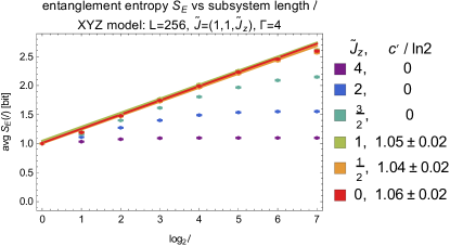
As shown in Fig. 4, in the spin glass phases, the entanglement entropy $S_{\text{E}}$ asymptotes to a constant with increasing subsystem length $\ell$ since it is a short range correlated phase. Furthermore, $S_{\text{E}}\geq\ln 2$ due to the spin glass order. These results can be understood deep in the spin glass phase via the LIOM in Eq. (31) from the stabilizer rank algorithm. Fattal et al. (2004); You et al. (2015) See Appendix E for details.

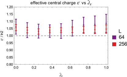
In the critical phases, the entanglement entropy $S_{\text{E}}$ appears to diverge logarithmically with subsystem length $\ell$ (Fig. 4):

$$S_{\text{E}}(\ell) =\frac{c^{\prime}}{3}\ln\ell$$ (8)

$$c^{\prime} =\ln 2$$

The constant $c^{\prime}$ is the effective central charge, which is postulated to be related to the central charge $c$ without disorder by $c^{\prime}=c\ln 2$ Refael and Moore (2004) (for Ising and Heisenberg types of models). Without disorder, the XYZ model has $c=1$ in the critical phase, and so we expect and observe $c^{\prime}=\ln 2$ in our disordered model (Fig. 4). The logarithmically diverging entanglement entropy in Eq. (8) is a result of the LIOM becoming nonlocal (see Fig. 11). This causes more LIOM to be cut by the subsystem $A$ and enter the entanglement entropy equation Eq. (32).

V Edwards-Anderson Correlator

A common approach to characterize glassy order is the Edwards-Anderson correlator. The disorder and energy averaged Edwards-Anderson spin glass correlator of $\sigma_{0}^{\mu}\sigma_{x}^{\mu}$ is defined to be

$$\text{avg}\langle\sigma_{0}^{\mu}\sigma_{x}^{\mu}\rangle^{2}\equiv\frac{1}{N_{\delta}}\sum_{\delta}\frac{1}{N_{E}}\sum_{E}\langle E|\sigma_{0}^{\mu}\sigma_{x}^{\mu}|E\rangle^{2}_{\delta}$$ (9)

It is the average of the square of $\langle\sigma_{0}^{\mu}\sigma_{x}^{\mu}\rangle$ over disorder configurations ($\delta$) and energies ($E$). $\sigma_{0}^{\mu}$ and $\sigma_{x}^{\mu}$ are Pauli matrices at lattice sites $0$ and $x$, respectively. We average over all energy eigenstates because we’re interested in the entire spectrum of states. Additionally, in the strong disorder limit, the LIOM take the form of products of Pauli matrices, and the eigenstates of these LIOM (and the Hamiltonian) all have the same Edwards-Anderson Correlators.

Figure 5: Disorder and energy averaged Edwards-Anderson $\sigma^{x}\sigma^{x}$ (top) and $\sigma^{z}\sigma^{z}$ (bottom) correlators (Eq. (9)) vs distance $x$ for different $\tilde{J}_{z}$ in the XYZ spin chain with $\tilde{J}_{x}=\tilde{J}_{y}=1$ and system size $L=256$. When $\tilde{J}_{z}>1$, the system is a $\sigma^{z}\sigma^{z}$ spin glass phase, and the $\sigma^{x}\sigma^{x}$ correlator decays exponentially while the $\sigma^{z}\sigma^{z}$ correlator asymptotes to a constant. When $\tilde{J}_{z}$ is only slightly larger than 1, e.g. $\tilde{J}_{z}=3/2$, there appears to be moderate finite size effects. When $\tilde{J}_{z}<1$, the system is critical with power law $\sigma^{\mu}\sigma^{\mu}$ correlators ($\mu$ summation not implied) with critical exponents $\eta_{xy}$ and $\eta_{z}$ (Eq. (10), Fig. 6), which were calculated using the slope of the fit to the $x=\frac{1}{2}\sqrt{L}-1,\sqrt{L}-1,2\sqrt{L}-1$ data points. (error bar details: foo )

Figure 6: Critical exponents $\eta_{xy}$ and $\eta_{z}$ (Eq. (10)) vs $\tilde{J}_{z}$ with $\tilde{J}_{x}=\tilde{J}_{y}=1$ for the XYZ spin chain of various system sizes $L$. $\eta_{xy}$ ($\eta_{z}$) appears to increase (decrease) continuously as $\tilde{J}_{z}$ increases. At least for $\tilde{J}_{z}>1/2$, we do not expect the continuously varying exponents to be a result of finite size effects because $\eta$ shows very little system size dependence in the above plot. The critical exponents were calculated as shown in Fig. 5. (error bar details: foo )

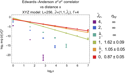
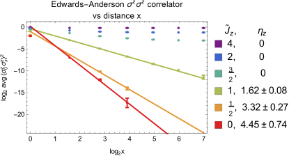
If $\tilde{J}_{z}>\tilde{J}_{x}$ and $\tilde{J}_{z}>\tilde{J}_{y}$, the system is in a $\sigma^{z}\sigma^{z}$ spin glass phase and the $\sigma^{z}\sigma^{z}$ Edwards-Anderson correlator (Eq. (9)) asymptotes to a constant for large distance $x$ (with exponentially small corrections) (Fig. 5). Physically, this implies that $\sigma_{i}^{z}\sigma_{j}^{z}$ has developed a finite overlap with products of the local integrals of motion (LIOM) (Eq. (12)) of the MBL phase, and is thus roughly conserved. However, the $\sigma^{x}\sigma^{x}$ and $\sigma^{y}\sigma^{y}$ correlators decay exponentially with distance $x$, as expected.

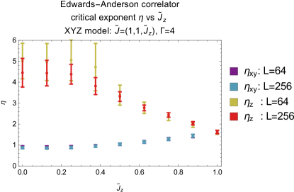
When $\tilde{J}_{z}<\tilde{J}_{x}=\tilde{J}_{y}$, the system is in a marginal MBL critical phase between $\sigma^{x}\sigma^{x}$ and $\sigma^{y}\sigma^{y}$ spin glasses (Fig. 1). The spin configuration in the marginal MBL state is dominated by nested domains of $\sigma^{x}\sigma^{x}$ and $\sigma^{y}\sigma^{y}$ Ising spin glass orders. The domains have fractal structures throughout the lattice, leading to the power-law decay of $\sigma^{\mu}\sigma^{\mu}$ Edwards-Anderson correlators ($\mu$ summation not implied) with critical exponents $\eta_{xy}$ and $\eta_{z}$ (Fig. 6):

$$\text{avg}\langle\sigma_{0}^{x}\sigma_{x}^{x}\rangle^{2} =\text{avg}\langle\sigma_{0}^{y}\sigma_{x}^{y}\rangle^{2}\sim x^{-\eta_{xy}}$$

$$\text{avg}\langle\sigma_{0}^{z}\sigma_{x}^{z}\rangle^{2} \sim x^{-\eta_{z}}$$ (10)

Unlike the effective central charge $c^{\prime}$ (Eq. (8)) which remains fixed, $\eta_{xy}$ ($\eta_{z}$) appears to increase (decrease) continuously with increasing $\tilde{J}_{z}$. The power-law decay of $\sigma^{z}\sigma^{z}$ can be understood in the limit $J_{z}=0$, where the system can be mapped to two independent free random Majorana fermion chains.

VI Long Range Mutual Information

Figure 7: Disorder and energy averaged long range mutual information (LRMI) $\mathcal{I}$ of two subsystems (of length $\ell=1$ (top) and $\ell=4$ (middle)) vs subsystem separation $x$ for different $\tilde{J}_{z}$ in the XYZ spin chain with $\tilde{J}_{x}=\tilde{J}_{y}=1$ and system size $L=256$. Subsystem length $\ell$ and separation $x$ are defined as shown in the bottom diagram. When $\tilde{J}_{z}>1$, the system is in a spin glass phase, and the LRMI asymptotes to a constant. When $\tilde{J}_{z}$ is only slightly larger than 1, e.g. $\tilde{J}_{z}=3/2$, there appears to be moderate finite size effects. When $\tilde{J}_{z}\leq 1$, the system is in a marginal MBL phase, and the LRMI decays according to a power law with a critical exponent $\kappa$: $\mathcal{I}_{\ell}(x)\sim(x/\ell)^{-\kappa}$. The critical exponent $\kappa$ does not appear to depend on the subsystem length $\ell$, but it does appear to increase continuously with $\tilde{J}_{z}$, unlike the effective central charge $c^{\prime}$ which remains fixed (Fig. 4). If the above plots were drawn on top of each other, the critical $\tilde{J}_{z}\leq 1$ data would very nearly overlap, which implies that changing $\ell$ just rescales $x$ as one would expect in a scale invariant system: $\mathcal{I}_{\ell}(x/\ell)\approx\mathcal{I}_{\ell^{\prime}}(x/\ell^{\prime})$. (error bar details: foo )

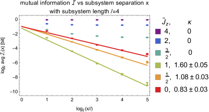
In Sec. IV we used the entanglement entropy to diagnose the critical phase as a marginal MBL phase due to its logarithmically diverging entanglement entropy (Eq. (8)). However, only studying the asymptotics of the entanglement entropy $S_{\text{E}}(\ell)$ for large connected subsystem has some limitations. For example, $S_{\text{E}}(\ell)$ can not firmly distinguish a trivial phase from a spin glass, since both just asymptote to a constant. Instead of studying the entanglement entropy of just a single connected subsystem, it has been proposed to study the long range mutual information (LRMI) between two disconnected subsystems with large separation Jian et al. (2015). The mutual information $\mathcal{I}$ between two non-overlapping subsystems $A$ and $B$ is defined to be

$$\mathcal{I}(A,B)=S_{\text{E}}(A)+S_{\text{E}}(B)-S_{\text{E}}(A\cup B)$$ (11)

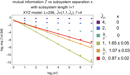
We will take subsystems $A$ and $B$ to be lines of length $\ell$ with separation given by $x$ as shown in Fig. 7 (bottom). We will be interested in the $L=\infty$ limit of the asymptotics of the LRMI $\mathcal{I}_{\ell}(x)$ as the separation $x$ tends to infinity while the subsystem length $\ell$ is held fixed. Since the mutual information is also an upper bound of correlation functions, in principle, the mutual information should decay slower than any correlation function.

In a direct product state with no spin glass order (which doesn’t exist in the XYZ model), far apart regions share little entanglement, and thus the LRMI should decay exponentially. In a spin glass phase there is long range glassy order, and the LRMI asymptotes to a constant (Fig. 7). Thus, LRMI can easily distinguish a trival phase from a spin glass phase. This fact could be very useful in more complicated models where finding the right order parameter is difficult. Finally, in a critical phase in any dimension, the LRMI is expected to decay according to a power law with some critical exponent $\kappa$: $\mathcal{I}_{\ell}(x)\sim(x/\ell)^{-\kappa}$. In the XYZ model, a power law is indeed observed (Fig. 7). Since the mutual information should not decay faster than the correlation functions, we at least expect $\kappa\leq\min(\eta_{xy},\eta_{z})$, which is also verified within the numerical error. The critical exponent $\kappa$ does not seem to depend on the subsystem length $\ell$; but $\kappa$ does appear to increase continuously with $\tilde{J}_{z}$, unlike the effective central charge $c^{\prime}$ which remains fixed. Thus, the LRMI can efficiently tell if a phase is a trivial, spin glass, or marginal MBL critical phase; and works as expected in the XYZ model (Fig. 7).

VII Conclusion

In conclusion, we have studied the XYZ spin chain with independently random XX, YY, and ZZ couplings on each bond. Unlike the random XXZ or Heisenberg models, the XYZ model breaks the continuous spin rotational symmetry down to the discrete $\mathbb{Z}_{2}^{2}$ symmetry, such that the quantum phase transitions between different symmetry-breaking spin glass phases can persist to finite energy density as marginal MBL critical lines. We use the SBRG numerical method to calculate the entanglement entropy, Edwards-Anderson correlator, and long-range mutual information. In the MBL spin glass phase, the entanglement entropy follows the area-law scaling and quickly saturates to a value of $S_{\text{E}}\geq\ln 2$. Both the Edwards-Anderson correlator and the long-range mutual information exhibit long-range behavior, demonstrating spin glass order. Along the marginal MBL critical line, the entanglement entropy follows the logarithmic scaling $S_{\text{E}}(\ell)=(c^{\prime}/3)\ln\ell$, with a fixed effective central charge $c^{\prime}=\ln 2$. Both the Edwards-Anderson correlator and the long-range mutual information decays in a power-law, and the critical exponents varies continuously along the marginal MBL line.

Appendix A Many Body Localization

A Hamiltonian is said to be fully many body localized (MBL) if all eigenstates in the many-body spectrum are localized Nandkishore and Huse (2015). It is believed that there exists a finite local unitary transformation $U$ that can diagonalize the MBL Hamiltonian $H$:

$$H_{\text{eff}} =UHU^{\dagger}$$ (12)

$$=\sum_{i}h_{i}^{(1)}\tau_{i}^{z}+\sum_{ij}h_{ij}^{(2)}\tau_{i}^{z}\tau_{j}^{z}+\sum_{ijk}h_{ijk}^{(3)}\tau_{i}^{z}\tau_{j}^{z}\tau_{k}^{z}+\cdots$$

where the $\tau_{i}^{z}$ are the LIOM. The fact that $U$ is a finite local unitary transformation means that it can be written as a finite time evolution of a time dependent local Hamiltonian with bounded spectrum. This implies that the LIOM $U\tau_{i}^{z}U^{\dagger}$ must be local operators (with exponentially decaying tails). This implies that the eigenstates of an MBL Hamiltonian display an area law entanglement (Fig. 4), as opposed to the volume law seen in excited states of thermal systems. An example of such a $U$ can be inferred from Fig. 12. Furthermore, the $h_{ijk\dots}^{(n)}$ decay exponentially with $n$ (Fig. 3) and distance $\max(|i-j|,|i-k|,|j-k|,\dots)$. This implies that in an MBL system, the time evolution of a direct product state displays an entanglement entropy which increases only logarithmically with time Serbyn et al. (2013b); Bardarson et al. (2012); Žnidarič et al. (2008), instead of linearly as in thermal systems. This implies that an MBL system can’t efficiently spread entanglement, and thus can’t act as its own heat bath.

A.1 Marginal MBL

If one observes a phase transition between two fully MBL phases, then it’s possible that the critical point between them is a marginal MBL phase. A margin MBL phase doesn’t obey Eq. (12) with the same restrictions for the unitary transformation $U$ and coefficients $h_{ijk\dots}^{(n)}$. For example, the LIOM in the original bases $U\tau_{i}^{z}U^{\dagger}$ become nonlocal You et al. (2015), which implies that $U$ can’t be a finite local unitary transformation. In SBRG, the unitary transformation $U$ that is found is nonlocal and requires a time evolution that diverges logarithmically with the system size, as can be inferred from Fig. 11.

Appendix B Spectrum Bifurcation Renormalization Group

In this work, we use the recently developed Spectrum Bifurcation Renormalization Group (SBRG) You et al. (2015) to simulate the XYZ model. SBRG is similar to RSRG-X Pekker et al. (2014), and behaves similarly to RSRG-X for the models on which RSRG-X can be applied. However, SBRG differs in that it (approximately) computes the commuting local integrals of motion (LIOM) (also know as localized-bit Huse et al. (2014) stabilizers) of a Hamiltonian, and therefore targets the entire spectrum at once; while RSRG-X targets a specific eigenstate energy at a time. That is, given an arbitrary local Hamiltonian $H$ written in terms of physical spins $\sigma_{i}^{\mu}$, SBRG computes the unitary transformation $U$ to a set of LIOM Pauli operators $\tau_{i}^{\mu}$ such that $H$ can be written as the sum of products of commuting $\tau_{i}^{z}$ operators with coefficients ($h_{i}^{(1)},h_{ij}^{(2)},h_{ijk}^{(3)},...$) as in Eq. (12). The unitary transformation $U$ is encoded using alternating $C_{4}$ transformations (see end of Appendix B.1) and small Schrieffer-Wolff perturbations (Eq. (16)).

With this information, SBRG can efficiently compute many quantities of interest such as Edwards-Anderson spin glass order parameters, the energy spectrum, entanglement entropies, and other LIOM properties. One advantage of SBRG is that it can handle Hamiltonian terms which are arbitrary local products of sigma matrices. This should be contrasted with other real space RG schemes (such as RSRG-X Pekker et al. (2014)) which require a specific Hamiltonian that is of closed form under RG. For example, next nearest neighbor terms often are not allowed to be created by the RG step of other methods. This flexibility allows SBRG to be applied to a large class of spin systems in all dimensions, including systems with topological order and symmetry protected topological order.

However, the price paid for this generality is that the Hamiltonian is not of closed form under RG, which results in exponentially many terms generated by the RG flow. Many of these terms will need to be dropped in order to preform computations efficiently. In this work, up to 256 addition off-diagonal terms are allows to be added during each RG step. This approximation seems to work well for systems with large disorder and deep in the fully MBL phase; but in marginal MBL phases, very large system sizes can become problematic. However, for the XYZ chain, it appears that reasonably accurate simulations can still be performed for systems of roughly 256 spins in the marginal MBL phase, and at least 10,000 spins deep in the MBL phase.

B.1 RG Step and Approximations

In SBRG, the Hamiltonian of a system is written as a linear combination of tensor products of pauli matrices:

$$H=\sum_{[\mu]}h_{[\mu]}\sigma^{[\mu]}=\sum_{[\mu]}h_{[\mu]}\otimes_{i}\sigma^{\mu_{i}}$$ (13)

As described in Appendix A2 of You et al. (2015), for each RG step, the term $h_{3}\sigma^{[\mu_{3}]}$ with the largest coefficient $h_{3}$ is chosen to be the next local integral of motion (LIOM) since it describes the leading energy scale. However, $\sigma^{[\mu_{3}]}$ doesn’t yet commute with the Hamiltonian $H$. The Hamiltonian can be split into three parts

$$H=h_{3}\sigma^{[\mu_{3}]}+\Delta+\Sigma$$

where $\Delta$ commutes with $\sigma^{[\mu_{3}]}$ while $\Sigma$ anticommutes with $\sigma^{[\mu_{3}]}$. In order to make $\sigma^{[\mu_{3}]}$ into a LIOM, we must eliminate $\Sigma$. First assume that

$$|\Sigma| \ll h_{3}$$ (14)

$$\max_{\Delta_{0}\in\Delta,[\Sigma,\Delta_{0}]\neq 0}|\Delta_{0}| \ll h_{3}$$ (15)

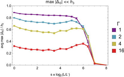
where $|\Sigma|\equiv\sqrt{2^{-L}\,\mathrm{Tr}(\Sigma\cdot\Sigma^{\dagger})}$ and $\max_{\Delta_{0}\in\Delta,[\Sigma,\Delta_{0}]\neq 0}|\Delta_{0}|$ is the absolute value of the largest pauli matrix coefficient of all terms in $\Delta$ that don’t commute with $\Sigma$. Fig. 8 provides evidence that these assumptions are valid. (RSRG-X depends on a similar set of assumptions.) With these assumptions, a Schrieffer-Wolff transformation can be performed in order to eliminate the off-diagonal component $\Sigma$ to order $O(h_{3}^{-2})$:

$$S =\exp\left(-\frac{1}{2h_{3}}\sigma^{[\mu_{3}]}\Sigma\right)$$ (16)

$$=1-\frac{1}{2h_{3}}\sigma^{[\mu_{3}]}\Sigma-\frac{1}{8h_{3}^{2}}\Sigma^{2}+O(h_{3}^{-3})$$

$$H \rightarrow H^{\prime}=S^{\dagger}HS$$

$$=h_{3}\sigma^{[\mu_{3}]}+\Delta+\frac{1}{2h_{3}}\sigma^{[\mu_{3}]}\Sigma^{2}$$ (17)

$$+\frac{1}{2h_{3}}\sigma^{[\mu_{3}]}[\Sigma,\Delta]+O(h_{3}^{-2})$$

The first approximation (Eq. (14)) allows the unitary $S$ to be expanded and implies that the third term in $H$ is small: $\frac{1}{2h_{3}}\sigma^{[\mu_{3}]}\Sigma^{2}\sim O(h_{3}^{-1})$. Although the first three terms of $H^{\prime}$ (Eq. (17)) commute with $\sigma^{[\mu_{3}]}$, the final term ($\frac{1}{2h_{3}}\sigma^{[\mu_{3}]}[\Sigma,\Delta]$) does not. This term must be removed since it’s $O(h_{3}^{-1})$, which is the leading order in the new terms that are generated by the RG step. However, this term can be ignored since another unitary transformation can eliminate it at the expense of only $O(h_{3}^{-2})$ terms:

$$H^{\prime} \rightarrow H^{\prime\prime}=U^{\dagger}HU$$

$$=h_{3}\sigma^{[\mu_{3}]}+\Delta+\frac{1}{2h_{3}}\sigma^{[\mu_{3}]}\Sigma^{2}+O(h_{3}^{-2})$$ (18)

The second approximation (Eq. (15)) is used to to claim that the last term in Eq. (17) is indeed $O(h_{3}^{-1})$.

Thus, $\sigma^{[\mu_{3}]}$ is a LIOM of $H^{\prime\prime}$ at order $O(h_{3}^{-2})$ if we can assume Eq. (14) and 15. In Fig. 8 we show that these appear to be safe and controlled approximations for sufficiently large $\Gamma$ in the critical phase. (The approximations are even better in the spin glass phase.) The first approximation (Eq. (14)) gets better under RG flow, while the second (Eq. (15)) does not show a clear trend. If the second approximation is actually getting worse under RG, this might suggest that the critical phase in the XYZ model is actually thermal.

Now that $\sigma^{[\mu_{3}]}$ commutes with the Hamiltonian, we may want to perform a change of basis $\sigma^{[\mu_{3}]}\rightarrow\tau^{3}_{j}$. Any integer $j$ can be used as long as it hasn’t been used before. E.g. $j$ could be chosen to indicate the RG step number, or the rough position of $\sigma^{[\mu_{3}]}$ on the lattice. In practice, it is convenient to use the same Hilbert space for $\sigma$ and $\tau$. This can be done by rotating $\sigma^{[\mu_{3}]}\rightarrow\sigma^{3}_{j}$ using a unitary transformation composed of one or two $C_{4}$ transformations $\exp\left(\frac{\mathrm{i}\pi}{4}\sigma^{[\mu]}\right)$ as described in You et al. (2015).

Figure 8: Disorder average of $|\Sigma|/h_{3}$ (Eq. (14)) (top) and $\max|\Delta_{0}|/h_{3}$ (Eq. (15)) (bottom) vs amount of RG flow $s\equiv\log_{2}(L/L^{\prime})$ for different amounts of disorder $\Gamma$ where $L=256$ is the system size and $L^{\prime}$ is the number of remaining spins. These are the small parameters used in the approximations Eq. (14) and 15. Data is shown at the critical point $\tilde{J}_{x}=\tilde{J}_{y}=\tilde{J}_{z}=1$; away from this point, these approximations are even better. As the disorder $\Gamma$ increases, the plotted values get arbitrarily small, suggesting that these approximations can be controlled by $\Gamma$. In addition, the first approximation (top) gets better under RG flow (for large $\Gamma$); the second (bottom) does not show a clear trend. Similar to Fig. 3, the large $\Gamma$ data in this plot can also be collapsed to a single curve if $f(y)=y^{1/\Gamma}$ is applied to the data, which shows that $|\Sigma|\sim\max|\Delta_{0}|\sim e^{-\Gamma}$ decreases exponentially as $\Gamma$ increases. (error bar details: foo )

B.2 Edwards-Anderson Correlator via SBRG

Given a Hamiltonian $H$, SBRG calculates the Schrieffer-Wolff transformation $S_{\text{tot}}=\prod S_{j}$ (Eq. (16)) that rotates (Eq. (20)) the Hamiltonian into a basis with LIOM $\sigma^{[\mu_{3}]}_{j}$. Before applying $S_{\text{tot}}$, $\sigma^{[\mu_{3}]}_{j}$ are only approximate LIOM of $H$.

We want to calculate the energy averaged Edwards-Anderson correlator of an operator $Q$:

$$\text{avg}\langle Q\rangle^{2}\equiv\frac{1}{N_{E}}\sum_{E}\langle E|Q|E\rangle^{2}$$ (19)

To do this, we will apply the Schrieffer-Wolff transformation to both $\sigma^{[\mu]}$ and $|E\rangle$:

$$H\rightarrow\tilde{H} \equiv S_{\text{tot}}^{\dagger}HS_{\text{tot}}$$ (20)

$$|E\rangle\rightarrow|\tilde{E}\rangle \equiv S_{\text{tot}}^{\dagger}|E\rangle$$ (21)

$$Q\rightarrow\tilde{Q} \equiv S_{\text{tot}}^{\dagger}QS_{\text{tot}}$$ (22)

$$=\sum_{[\mu]}q_{[\mu]}\sigma^{[\mu]}$$

for some set of coefficients $q_{[\mu]}$. Now every $\sigma^{[\mu_{3}]}_{j}$ takes a definite value for every energy eigenstate $|\tilde{E}\rangle$ of $\tilde{H}$: $\sigma^{[\mu_{3}]}_{j}=\pm 1$. This implies that $\langle\tilde{E}|\sigma^{[\mu]}|\tilde{E}\rangle=\pm 1$ if $\sigma^{[\mu]}$ commutes with all $\sigma^{[\mu_{3}]}_{j}$, otherwise it’s zero. Thus

$$\text{avg}\langle Q\rangle^{2} =\frac{1}{N_{E}}\sum_{E}\langle\tilde{E}|\tilde{Q}|\tilde{E}\rangle^{2}$$ (23)

$$=\frac{1}{N_{E}}\sum_{E}\sum_{[\mu]}\langle\tilde{E}|q_{[\mu]}\sigma^{[\mu]}|\tilde{E}\rangle^{2}$$

$$=\sum_{[\mu]}\left\{\begin{array}[]{ll}q_{[\mu]}^{2}&\sigma^{[\mu]}\text{ commutes with all }\sigma^{[\mu_{3}]}_{j}\\ 0&\text{otherwise}\end{array}\right.$$ (26)

In the second line, we were able to pull the $\sum_{[\mu]}$ out of $\langle\tilde{E}|\cdots|\tilde{E}\rangle^{2}$ because cross terms cancel after the energy average. Thus, the energy averaged Edwards-Anderson correlator can be calculated from the coefficients $q_{[\mu]}$ of $\tilde{Q}$ (Eq. (22)).

B.3 Algorithm and Implementation Details

Unfortunately, the Schrieffer-Wolff transformation generates an exponentially large number of terms in $\Sigma^{2}$ in Eq. (18) and $\tilde{Q}$ in Eq. (22). Thus, one must drop terms. In this work, for each Schrieffer-Wolff transformation, we keep the 256 largest additional terms in $\Sigma^{2}$ and 32 largest additional terms in $\tilde{Q}$.

Most operators $\sigma^{[\mu]}$ in the Hamiltonian will be local. Thus, it is important to make use of this locality when implementing SBRG. With this optimization, the CPU time for an SBRG simulation of a Hamiltonian in an MBL phase scales linearly (up to log corrections) with system size.

For this work, each $L=256$ disorder realization data point took a couple minutes of CPU time. However, reasonable data is achievable with only 1/8th as many additional terms in $\Sigma^{2}$ and $\tilde{Q}$, for which a simulation only takes several seconds. The SBRG data used in this paper was calculated in roughly two weeks on a quad-core i7-3720QM underclocked to 2GHz. The SBRG data included 1024 disorder realizations for each data point. However, reasonable data was attainable with less ($\sim 100$) disorder realizations and additional terms, for which only a few hours of simulation time is necessary.

For this work, the Haskell programming language was used to implement SBRG in roughly 1000 lines of code, and the implementation has been published to github Slagle (2016). Haskell was chosen because it could produce fast code (potentially faster than C++ due to very efficient garbage collection) while requiring the smallest amount of developer time compared to other languages. Development time was minimized using Haskell because Haskell is very good at dealing with complicated data structures, which were necessary for making use of the locality of operators mentioned above. This is a result of Haskell’s strong type system, automatic garbage collection, functional programming paradigm, and high amount of expressiveness.

Random numbers were generated using a combined linear congruential generator (System.Random.StdGen in Haskell) with period $2^{61}$, which is much larger than the number of random numbers used in this work, which was roughly $2^{29}$.

Appendix C XYZ Model Details

C.1 Disorder Distribution

SBRG is a numerical method which relies on large disorder for accuracy. For this reason, it is important that we choose a disorder distribution with very large randomness. For the XY ($J_{z}=0$) and XXZ ($J_{i,x}=J_{i,y}$) spin chains, it has been shown that with large disorder, $J_{i,\mu}$ flows to a power law distribution Fisher (1992, 1994) with a probability distribution function (PDF) equal to

$$\mathrm{PDF}(J_{i,\mu})=\frac{1}{\Gamma J_{i,\mu}}\left(\frac{J_{i,\mu}}{J_{\mu}}\right)^{1/\Gamma}\quad,\quad J_{i,\mu}>0$$ (27)

where $\Gamma$ controls the strength of the disorder, with larger $\Gamma$ corresponding to stronger disorder. It’s useful to define $\beta_{i,\mu}\equiv-\ln\frac{J_{i,\mu}}{J_{\mu}}\geq 0$. With this definition, $\beta_{i,\mu}$ follows an exponential distribution with a mean and standard deviation (as in Eq. (1)) equal to $\Gamma$:

$$\mathrm{PDF}(\beta_{i,\mu})=\Gamma^{-1}e^{-\beta_{i,\mu}/\Gamma}\quad,\quad\beta_{i,\mu}>0$$ (28)

It’s also useful to define $\tilde{J}_{i,\mu}$ by $J_{i,\mu}\equiv\tilde{J}_{i,\mu}^{\Gamma}$. With this definition, $\tilde{J}_{i,\mu}$ is uniformly distributed in $[0,\tilde{J}_{\mu}]$ where $J_{\mu}\equiv\tilde{J}_{\mu}^{\Gamma}$:

$$\mathrm{PDF}(\tilde{J}_{i,\mu})=\tilde{J}_{\mu}^{-1}\quad,\quad 0<\tilde{J}_{i,\mu}<\tilde{J}_{\mu}$$ (29)

We therefore let $J_{i,\mu}$ follow the above (equivalent) distributions so that we can effectively probe closer to the infinite system size limit while using the same physical system size. (We assume that the disorder becomes stronger under RG in the large disorder limit.) We will show results for $\Gamma=4$ because this is the smallest $\Gamma$ for which SBRG agrees well with exact diagonalization on small latices (data not shown in this paper), and for which our approximations appear to be safe (see Appendix B.1 and D, and Sec. III.2).

C.2 Tuning Parameters

We use $\tilde{J}_{\mu}$ as tuning parameters instead of $J_{\mu}$ because $\tilde{J}_{\mu}$ are better behaved at large disorder $\Gamma$. For example, our phase diagram in Fig. 1 would depend strongly on $\Gamma$ if $J_{\mu}$ were used as tuning parameters instead of $\tilde{J}_{\mu}$. However, when $\tilde{J}_{\mu}$ are used as tuning parameters, the phase diagram has little dependence on $\Gamma$ when $\Gamma$ is large; and this allows the large disorder limit to be well defined.

A simple calculation makes this more transparent. If $P(J_{i,\mu}>J_{i,\nu})$ is the probability that $J_{i,\mu}>J_{i,\nu}$, then $P(J_{i,\mu}>J_{i,\nu})\rightarrow\frac{1}{2}$ as $\Gamma\rightarrow\infty$ if $J_{\mu}$ is held constant. Thus large disorder effectively washes out the differences between different $J_{\mu}$ and the $J_{1}=J_{2}=J_{3}$ point effectively dominates the phase diagram if $J_{\mu}$ is held constant as $\Gamma\rightarrow\infty$. However, if we define $J_{\mu}\equiv\tilde{J}_{\mu}^{\Gamma}$ and hold $\tilde{J}_{\mu}$ constant instead, then $P(J_{i,\mu}>J_{i,\nu})$ is independent of $\Gamma$. This is because

$$P(J_{i,\mu}>J_{i,\nu}) =P(\tilde{J}_{i,\mu}>\tilde{J}_{i,\nu})\text{ since }J_{i,\mu}\equiv\tilde{J}_{i,\mu}^{\Gamma}$$

$$=\begin{cases}\;\;\;\frac{r}{2}&\text{if }r<1\\ 1-\frac{1}{2r}&\text{if }r>1\end{cases}\text{ by Eq.\,(\ref{eq:PDF tilde J})}$$

$$\quad\quad\text{where }r=\frac{\tilde{J}_{\mu}}{\tilde{J}_{\nu}}=\left(\frac{J_{\mu}}{J_{\nu}}\right)^{1/\Gamma}$$

Appendix D Exact Diagonalization Study

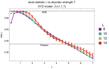
We now study the critical point $\tilde{J}_{x}=\tilde{J}_{y}=\tilde{J}_{z}=1$ using exact diagonalization to check that the critical phase is not thermal. In Fig. 9 we show the level statistic $r$ of the XYZ model vs disorder strength $\Gamma$. For each disorder realization, the level statistic $r_{n}^{(a)}$ is defined as a ratio of level spacings $\delta_{n}^{(a)}$ Oganesyan and Huse (2007) in a given symmetry sector $(a)$:

$$r_{n}^{(a)} \equiv\frac{\min(\delta_{n}^{(a)},\delta_{n+1}^{(a)})}{\max(\delta_{n}^{(a)},\delta_{n+1}^{(a)})}$$ (30)

$$\delta_{n}^{(a)} \equiv E_{n}^{(a)}-E_{n-1}^{(a)}$$

$$E_{n+1}^{(a)} \geq E_{n}^{(a)}$$

For our model, there are four symmetry sectors $(a)$ which are labeled by the eigenvalues of the symmetry operators of our model: $\prod_{i}\sigma_{i}^{x}$ and $\prod_{i}\sigma_{i}^{y}$. In Fig. 9 we average over disorder realizations, level spacings $n$, and symmetry sectors $(a)$. We find that with weak disorder $\Gamma$, the level statistic approaches (with increasing system size) the GOE (Gaussian orthogonal ensemble) level statistic $r_{\text{GOE}}\approx 0.53$, which is expected for a thermal system. As the disorder strength increases, the level statistic drops below the Poisson level statistic $r_{\text{Poisson}}\approx 0.39$, which suggests that the system is not thermal.

The level statistic continues below the Poisson level statistic because we use a power law distribution of coefficients in the Hamiltonian (Eq. (27)), instead of a uniform or Gaussian distribution. This can be understood most easily in the $\tilde{J}_{x}=\tilde{J}_{y}=0$ and $\tilde{J}_{z}=1$ limit (see Fig. 9), where the Hamiltonian is already diagonal. When $\Gamma=1$, we exactly reproduce the Poisson level statistic. However, a simple numerical calculation shows that as $\Gamma$ increases, the level statistic decays to zero as a power law with increasing $\Gamma$: $r\sim 1/\Gamma$.

In Fig. 10 we show the how the entanglement scales with subsystem size. When the disorder is weak, the system displays a volume law entanglement, as expected for a thermal system. But for strong disorder, the entanglement increases very slowly with subsystem size, which suggests that the strong disorder results in either a MBL phase with area law entanglement or a marginal MBL phase with log-law entanglement. (In Fig. 4 we SBRG and large system sizes to show that the entanglement follows a log-law.) Again we see that for weak disorder $\Gamma$, the critical point is thermal, but with strong disorder the critical point does not appear to be thermal.

It is worth emphasizing that in both ED plots, a disorder strength of $\Gamma=1$ (which corresponds to uniformly distributed random coefficients $J_{i}$) was not sufficient to prevent thermalization of the XYZ model’s critical point. Therefore, considering disordered systems with only Gaussian (with $\Gamma\approx 1.1$ via Eq. (1)) or uniform disorder distributions may not always be sufficient if one is interested in observing marginal MBL critical phases. That is, similar to the XYZ model’s critical point, other models may also require large $\Gamma$ (defined by Eq. (1)) in order to prevent thermalizaion.

Figure 9: Disorder and energy averaged level statistic $r$ (Eq. (30)) vs disorder strength $\Gamma$ for different system sizes $L$ in the XYZ spin chain with $\tilde{J}_{x}=\tilde{J}_{y}=\tilde{J}_{z}=1$. With weak disorder, the system approaches GOE level statistics with increasing system size, which indicates that the system is thermal. As the disorder strength increases, the level statistic drops below the Poisson level statistic, which suggests that the system is not thermal with strong disorder. (error bar details: foo )

Figure 10: Disorder and energy averaged entanglement entropy $S_{\text{E}}$ [bit] ($\equiv S_{\text{E}}/\ln 2$) (Eq. (6)) vs subsystem length $\ell$ for different disorder strengths $\Gamma$ in the XYZ spin chain with $\tilde{J}_{x}=\tilde{J}_{y}=\tilde{J}_{z}1$ and system size $L=2\ell$ with open boundary conditions. Each entanglement subsystem splits the system in half. We only show even $\ell$ in order to avoid an even-odd effect. As the disorder strength $\Gamma$ increases, the slope of the data decreases to roughly zero. This suggests a transition from a thermal phase with volume law entanglement to a non-thermal phase. (error bar details: foo )

Appendix E Spin Glass Entanglement Entropy Calculation

Here we calculate the entanglement entropy of a subsystem $A$ in the spin glass phase using the stabilizer rank algorithm in You et al. (2015). Deep in the spin glass phase where $J^{z}$ dominates, the LIOM are given by:

$$\tau_{i}^{z} =\sigma_{i}^{z}\sigma_{i+1}^{z}\text{ with }i=1,2,\ldots L-1$$ (31)

$$\tau_{L}^{z} =\prod_{i=1}^{L}\begin{cases}\sigma^{x}&\text{if }J_{x}>J_{y}\\ \sigma^{y}&\text{if }J_{y}>J_{x}\end{cases}$$

Assuming $i<j$. We can see that in this case indeed $\sigma_{i}^{z}\sigma_{j}^{z}=\prod_{k=i}^{j-1}\tau_{k}^{z}$ is a product of the LIOM. Only three of the LIOM will be cut by the subsystem $A$, which we will take to be the sites $i,i+1,\ldots j$ where $j=i-1+\ell$. These LIOM are $\tau_{i-1}^{z},\tau_{j}^{z},\tau_{L}^{z}$. We then “trace out degrees of freedom not in $A$” by removing $\sigma$-matrices not in $A$:

$$\tau_{i-1}^{z} =\sigma^{z}_{i-1}\sigma^{z}_{i} \tau_{j}^{z} =\sigma^{z}_{j}\sigma^{z}_{j+1} \tau_{L}^{z} =\prod_{i^{\prime}}\sigma^{x}_{i^{\prime}}$$

$$\downarrow \downarrow \downarrow$$

$$\hat{\tau}_{i-1}^{z} \rightarrow\sigma^{z}_{i} \hat{\tau}_{j}^{z} \rightarrow\sigma^{z}_{j} \hat{\tau}_{L}^{z} \rightarrow\prod_{i^{\prime}=i}^{j}\sigma^{x}_{i^{\prime}}$$

We then consider the 3x3 anticommutivity matrix of these three $\hat{\tau}$ operators:

$$M=\left(\begin{smallmatrix}0&0&1\\ 0&0&1\\ 1&1&0\end{smallmatrix}\right)$$

where a $1$ denotes anticommutivity while a $0$ denotes commutivity. The entanglement entropy $S_{\text{E}}$ is then given by

$$S_{\text{E}} =\frac{\ln 2}{2}\text{rank}M\text{ (over $\mathbb{Z}_{2}$)}$$ (32)

$$=\ln 2$$

where the matrix rank is calculated over the field $\mathbb{Z}_{2}$. When one isn’t deep in the spin glass phase, the LIOM become more complicated (as in Fig. 12); more LIOM are cut by $A$; and the entanglement entropy increases slightly due to additional boundary contributions which don’t depend significantly on the size of the subsystem $A$.

Figure 11: Approximate RG flow and LIOM for the XYZ spin chain at the critical point $\tilde{J}_{x}=\tilde{J}_{y}=\tilde{J}_{z}=1$. The initial Hamiltonian starts at the boundary of the disk, with a spin living at the end of each radial line at the edge of the disk. SBRG then performs an RG which identifies a LIOM at each step of the RG (see Appendix B.1). In the limit of large disorder, the LIOM can be approximated as a product of $\sigma^{x}$ (red), $\sigma^{y}$ (green), and $\sigma^{z}$ (blue) matrices (dots connected by an arc line in the figure). Each LIOM in the figure also marks the end of a radial line to denote that a degree of freedom has been diagonalized (cf. ”integrated out“) at this RG step. Because we are in a marginal MBL phase, LIOM exist with sizes at every length scale, which results in the critical properties of this phase: diverging entanglement entropy (Fig. 4), power-law Edwards-Anderson correlators (Fig. 5), and long power-law range mutual information (Fig. 7).

Figure 12: Approximate RG flow and LIOM for the XYZ spin chain in the spin glass phase with $\tilde{J}=(1,1,2)$. (See the caption of Fig. 11.) Because we are in the spin glass phase, the LIOM are dominated by blue $\sigma^{z}\sigma^{z}$ operators. The very large integral of motion in the center is just the $Z_{2}$ spin flip symmetry $\prod_{i}\sigma^{x}_{i}$, which is a little messy in the figure because it has been multiplied by some of the other LIOM to obtain an operator which is still an integral of motion. This center operator is essential for the spin glass properties of this phase: finite long range Edwards-Anderson correlators (Fig. 5) and finite long range mutual information (Fig. 7).