Galerkin method for the numerical solution of the Burgers’ equation by using exponential B-splines

Abstract

In this paper, the exponential B-spline Galerkin  method is set up for getting the numerical solution of the Burgers’ equation. Two numerical examples related to shock wave propogation and travelling wave are studied to illustrate the accuracy and the efficiency of the method. Obtained results are compared with some early studies.

Keywords: Exponential B-spline; Galerkin Method; Burgers’ equation.

1 Introduction

Burgers’ equation in which convection and diffusion play an important role arises in applications such as meteorology, turbulent flows, modelling of the shallow water. Burgers’ equation is considered to be useful model for many physically problems. Thus It is often studied for testing of both real life problems and computational techniques. Not only does exact solutions of nonlinear convective problem develops discontinuities in finite time, and might display complex structure near discontinuities. Efficient and accurate methods are in need to be tackled the complex solutions of the Burgers’ equation, as expected, many numerical researches are strived to beat difficulties. Though analytical solutions of the Burgers’ equation exist for simple initial condition , the numerical techniques are of interest to meet requirement of the wide range of solutions of the Burgers’ equations. Some variants of the Spline methods have set up to find the numerical solutions of the Burgers’ equations such as Galerkin finite element method [3, 9, 11, 12, 23], least square method [10], collocation method [8, 13, 14, 15, 16, 17, 22], finite difference method [1, 2], differential quadrature method [24, 25], method based on the cubic B-spline quasi interpolant [19, 20], Taylor–Galerkin and Taylor-collocation methods [21], etc.

Finite element methods are mainly used methods to have good functional solutions of the differential equations. The accuracy of the finite element solutions are increased by the selection of suitable basis function for the approximate function over the finite intervals. We will form the combination of the exponential B-spline as an approximate function for the finite element method to get the solution of the Burgers’ equation. The exponential B-splines are suggested to interpolate data and function exhibiting sharp variations [4, 5, 6, 7] since polynomial B-splines based interpolation cause unwanted osculation for interpolation. Some solutions of the Burgers’ equation show sharpness. Thus we will construct the finite element method together with the exponential B-splines to have solutions of the Burgers’ equation. Over the finite element, the Galerkin method will be employed to determine the unknown of the approximate solution. A few exponential B-spline numerical methods have suggested for some partial differential equations: Exponential B-spline collocation method is build up to compute numerical solution of the convection diffusion equation [26], the Korteweg-de Vries equation [27] and generalized Burgers-Fisher equation [28].

In this study, we will consider the Burgers’ equation

$$u_{t}+uu_{x}-\nu u_{xx}=0$$ (1)

where subscripts $x$ and $t$ are space and time parameters, respectively and $\nu$ is the viscosity coefficient. Boundary conditions of the Eq.(1) are chosen from

$$u\left(a,t\right)=\beta_{1},$$

(2)

and initial condition is

$$u\left(x,0\right)=f\left(x\right),x\in\left[a,b\right].$$ (3)

$f\left(x\right)$ and $\beta_{1},\beta_{2}$ constants are described in the computational section.

2 Exponential B-splines Galerkin Finite Element Solution

Divide spatial interval $[a,b]$ in $N$ subintervals of length $h=\dfrac{b-a}{N}$ and $x_{i}=x_{0}+ih$ at the knots $x_{i},$ $i=0,..,N$ and time interval $[0,T]$ in $M$ interval of length $\Delta t.$

Let $\phi_{i}\left(x\right)$ be the exponential B-splines defined at the knots $x_{i},$ $i=0,\ldots,N,$ together with fictitious knots $x_{i},$ $i=-3,-2,-1,N+1,N+2,N+3$ outside the interval $[a,b].$ The $\phi_{i}\left(x\right),$ $i=-1,\ldots,N+1$ can be defined as

$$\phi_{i}\left(x\right)=\left\{\begin{array}[]{lll}b_{2}\left[\left(x_{i-2}-x\right)-\dfrac{1}{p}\left(\sinh\left(p\left(x_{i-2}-x\right)\right)\right)\right]&\text{ \ }&\text{if }x\in\left[x_{i-2},x_{i-1}\right];\\ a_{1}+b_{1}\left(x_{i}-x\right)+c_{1}e^{p\left(x_{i}-x\right)}+d_{1}e^{-p\left(x_{i}-x\right)}&\text{ }&\text{if }x\in\left[x_{i-1},x_{i}\right];\\ a_{1}+b_{1}\left(x-x_{i}\right)+c_{1}e^{p\left(x-x_{i}\right)}+d_{1}e^{-p\left(x-x_{i}\right)}&\text{ }&\text{if }x\in\left[x_{i},x_{i+1}\right];\\ b_{2}\left[\left(x-x_{i+2}\right)-\dfrac{1}{p}\left(\sinh\left(p\left(x-x_{i+2}\right)\right)\right)\right]&\text{ }&\text{if }x\in\left[x_{i+1},x_{i+2}\right];\\ 0&\text{ }&\text{otherwise}\end{array}\right.$$ (4)

where

$$\begin{array}[]{l}p=\underset{0\leq i\leq N}{\max}p_{i},\text{ }s=\sinh\left(ph\right),\text{ }c=\cosh\left(ph\right),\\ a_{1}=\dfrac{phc}{phc-s},\text{ }b_{1}=\dfrac{p}{2}\left[\dfrac{c\left(c-1\right)+s^{2}}{\left(phc-s\right)\left(1-c\right)}\right],\text{ }b_{2}=\dfrac{p}{2\left(phc-s\right)},\\ c_{1}=\dfrac{1}{4}\left[\dfrac{e^{-ph}\left(1-c\right)+s\left(e^{-ph}-1\right)}{\left(phc-s\right)\left(1-c\right)}\right],\text{ }d_{1}=\dfrac{1}{4}\left[\dfrac{e^{ph}\left(c-1\right)+s\left(e^{ph}-1\right)}{\left(phc-s\right)\left(1-c\right)}\right].\end{array}$$

Each basis function $\phi_{i}\left(x\right)$ is twice continuously differentiable. Table 1 shows the values of $\phi_{i}\left(x\right),$ $\phi_{i}^{\prime}\left(x\right)$ and $\phi_{i}^{\prime\prime}\left(x\right)$ at the knots $x_{i}$:

Table 1: Exponential B-spline values

$$x_{i-2}$$

The $\phi_{i}\left(x\right),i=-1,\ldots,N+1$ form a basis for functions defined on the interval $[a,b]$. The Galerkin method consists of seeking approximate solution in the following form:

$$u\left(x,t\right)\approx U_{N}\left(x,t\right)=\overset{N+1}{\underset{i=-1}{\sum}}\phi_{i}\left(x\right)\delta_{i}\left(t\right)$$ (5)

where $\delta_{i}\left(t\right)$ are time dependent unknown to be determined from the boundary conditions and Galerkin approach to the equation (1). The approximate solution and the first two derivatives at the knots can be found from the Eq. (4-5) as

$$U_{i}=U_{N}(x_{i},t)=\alpha_{1}\delta_{i-1}+\delta_{i}+\alpha_{1}\delta_{i+1},$$

(6)

where $\alpha_{1}=\dfrac{s-ph}{2(phc-s)},\alpha_{2}=\dfrac{p(1-c)}{2(phc-s)},\alpha_{3}=\dfrac{p^{2}s}{2(phc-s)}.$

The approximate solution $U_{N}$ over the element $[x_{m},x_{m+1}]$ can be written as

$$U_{N}^{e} = \phi_{m-1}\left(x\right)\delta_{m-1}\left(t\right)+\phi_{m}\left(x\right)\delta_{m}\left(t\right)+\phi_{m+1}\left(x\right)\delta_{m+1}\left(t\right)$$ (7)

$$+\phi_{m+2}\left(x\right)\delta_{m+2}\left(t\right)$$

where quantities $\delta_{j}\left(t\right),j=m-1,...,m+2$ are element parameters and $\phi_{j}\left(x\right),j=m-1,...,m+2$ are known as the element shape functions.

Over the sample interval $[x_{m},x_{m+1}],$ applying Galerkin approach to Eq. (1) with the test function $\phi_{j}\left(x\right)$ yields the integral equation:

$$\underset{x_{m}}{\overset{x_{m+1}}{\int}}\phi_{j}\left(x\right)\left(u_{t}+uu_{x}-\nu u_{xx}\right)dx.$$ (8)

Substitution of the Eq. (7) into the integral equation lead to

$$\left.\overset{m+2}{\underset{i=m-1}{\sum}}\left(\underset{x_{m}}{\overset{x_{m+1}}{\int}}\phi_{j}\phi_{i}dx\right)\overset{\mathbf{\bullet}}{\delta}_{i}+\left(\underset{x_{m}}{\overset{x_{m+1}}{\int}}\phi_{j}\left(\overset{m+2}{\underset{k=m-1}{\sum}}\delta_{k}\phi_{k}\right)\phi_{i}^{\prime}dx\right)\delta_{i}\right.$$

$$\qquad\left.-\nu\left(\underset{x_{m}}{\overset{x_{m+1}}{\int}}\phi_{j}\phi_{i}^{\prime\prime}dx\right)\delta_{i},\right.$$ (9)

where $i,j$ and $k$ take only the values $m-1,m,m+1,m+2$ for $m=0,1,\ldots,N-1$ and $\overset{\mathbf{\bullet}}{}$ denotes time derivative.

If we denote $A_{ji}^{e},B_{jki}^{e}(\delta^{e})$ and $C_{ji}^{e}$ by

$$A_{ji}^{e}=\underset{x_{m}}{\overset{x_{m+1}}{\int}}\phi_{j}\phi_{i}dx,$$

(10)

where $\mathbf{A}^{e}$ and $\mathbf{C}^{e}$ are the element matrices of which dimensions are $4\times 4$ and $\mathbf{B}^{e}\left(\mathbf{\delta}^{e}\right)$ is the element matrix with the dimension $4\times 4\times 4$, Eq.(9) can be written in the matrix form as

$$\mathbf{A}^{e}\overset{\mathbf{\bullet}}{\mathbf{\delta}^{e}}+\left(\mathbf{B}^{e}\left(\mathbf{\delta}^{e}\right)-\nu\mathbf{C}^{e}\right)\mathbf{\delta}^{e},$$ (11)

where $\mathbf{\delta}^{e}\mathbf{=}\left(\delta_{m-1},...,\delta_{m+2}\right)^{T}.$

Gathering the systems (11) over all elements, we obtain global system

$$\mathbf{A}\overset{\mathbf{\bullet}}{\mathbf{\delta}}+\left(\mathbf{B}\left(\mathbf{\delta}\right)-\nu\mathbf{C}\right)\mathbf{\delta}=0$$ (12)

where $\mathbf{A},\mathbf{B}\left(\mathbf{\delta}\right),\mathbf{C}$ are derived from the corresponding element matrices $\mathbf{A}^{e},\mathbf{B}^{e}\left(\mathbf{\delta}^{e}\right),\mathbf{C}^{e}$, respectively and $\mathbf{\delta=}\left(\delta_{-1},...,\delta_{N+1}\right)^{T}$ contain all elements parameters.

The unknown parameters $\mathbf{\delta}$ are interpolated between two time levels $n$ and $n+1$ with the Crank-Nicolson method

$$\begin{array}[]{cc}\mathbf{\delta}=\dfrac{\mathbf{\delta}^{n+1}+\mathbf{\delta}^{n}}{2},&\overset{\mathbf{\bullet}}{\mathbf{\delta}}=\dfrac{\mathbf{\delta}^{n+1}-\mathbf{\delta}^{n}}{\Delta t},\end{array}$$

we obtain iterative formula for the time parameters $\mathbf{\delta}^{n}$

$$\left[\mathbf{A+}\frac{\Delta t}{2}\left(\mathbf{B}\left(\mathbf{\delta}^{n+1}\right)-\nu\mathbf{C}\right)\right]\mathbf{\delta}^{n+1}=\left[\mathbf{A-}\frac{\Delta t}{2}\left(\mathbf{B}\left(\mathbf{\delta}^{n}\right)-\nu\mathbf{C}\right)\right]\mathbf{\delta}^{n}.$$ (13)

The set of equations consist of $\left(N+3\right)$ equations with $\left(N+3\right)$ unknown parameters. Boundary conditions must be adapted into the system. Because of the this requirement, initially the first and last equations are eliminated from the (13) and parameters $\delta_{-1}^{n+1}$ and $\delta_{N+1}^{n+1}$ are substituted in the remaining system (13) by using following equations

$$\begin{array}[]{l}u\left(a,t\right)=\alpha_{1}\delta_{-1}^{n+1}+\delta_{0}^{n+1}+\alpha_{1}\delta_{1}^{n+1}=\beta_{1},\\ u\left(b,t\right)=\alpha_{1}\delta_{N-1}^{n+1}+\delta_{N}^{n+1}+\alpha_{1}\delta_{N+1}^{n+1}=\beta_{2}\end{array}$$

which are obtained from the boundary conditions. Thus we obtain a septa-diagonal matrix with the dimension $\left(N+1\right)\times\left(N+1\right)$. Since the system (13) is an implicit system together with the nonlinear term $\mathbf{B}\left(\mathbf{\delta}^{n+1}\right)$, we have used the following inner iteration at each time step $(n+1)\Delta t$ to work up solutions:

$$(\mathbf{\delta}^{\ast}\mathbf{)}^{n+1}=\mathbf{\delta}^{n}+\dfrac{(\mathbf{\delta}^{n}-\mathbf{\delta}^{n-1})}{2}.$$ (14)

We use the above iteration three times to find the new approximation $(\mathbf{\delta}^{\ast}\mathbf{)}^{n+1}$ for the parameters $\mathbf{\delta}^{n+1}$ to recover solutions at time step $(n+1)\Delta t$.

To start evolution of the iterative system for the unknown $\mathbf{\delta}^{n}$, the vector of initial parameters $\mathbf{\delta}^{0}$must be determined by using the following initial and boundary conditions:

$$u_{0}^{\prime}(x_{0},0)=\dfrac{p\left(1-c\right)}{2\left(phc-s\right)}\delta_{-1}+\dfrac{p\left(c-1\right)}{2\left(phc-s\right)}\delta_{1}$$

(15)

The solution of matrix equation (15) with the dimensions $\left(N+1\right)\times\left(N+1\right)$ is obtained by the way of Thomas algorithm. Once $\mathbf{\delta}^{0}$ is determined, we can start the iteration of the system to find the parameters $\mathbf{\delta}^{n}$ at time $t^{n}=n\Delta t.$ Approximate solutions at the knots is found from the Eq.(6) and solution over the intervals $[x_{m},x_{m+1}]$ is determined from the Eq.(7).

3 Test Problems

The robustness of the algorithm is shown by studying two test problems. Error is measured by the maximum error norm;

$$L_{\infty}=\left\|u^{\text{exact}}-u^{\text{numeric}}\right\|_{\infty}=\max_{0\leq j\leq N}\left|u_{j}^{\text{exact}}-u_{j}^{\text{numeric}}\right|.$$ (16)

The free parameter $p$ of the exponential B-spline is found by scanning the predetermined interval with very small increment.

(a) A shock propagation solution of the Burgers’ equation is

$$u(x,t)=\dfrac{x/t}{1+\sqrt{t/t_{0}}\exp(x^{2}/(4\nu t))},\text{\quad}t\geq 1,$$ (17)

where $t_{0}=\exp(1/(8\nu))$. The sharpness of the solutions increases with selection of the smaller $\nu$.

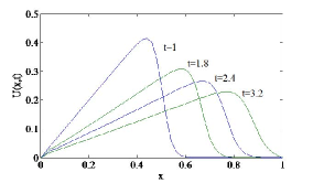
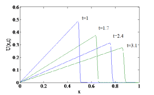
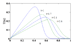
Substitution of the $t=1$ in Eq. (17) gives the initial condition. The boundary conditions $u(0,t)=0$ and $u(1,t)=0$ are used. Computations are performed with parameters $\nu=0.0005,$ $0.005,$ $0.01,$ $h=0.02,$ $0.005$ and $\Delta t=0.01$ over the solution domain $[0,1]$. As time increases, shock evaluation is observed and some graphical solutions are drawn in Figs. 1-3 for various viscosity values and space steps. For $\nu=0.01,$ algorithm produces smoother shock during run time. With decreasing values of $\nu$, as seen in the Figs. 1-3 the steepening occurs. For the smaller viscosity constant $\nu=0.0005$ the sharper shock is observed and steepness of numerical solution is kept almost unchanged during the program run. The results obtained by present scheme can be compared with ones given in the works [12, 14, 16, 17, 18] through the computation of $L_{\infty}$ error norm at various times in the Table 2.

Figure 1:  Solutions for $\nu=0.01\text{, }h=0.02$, $p=0.005111$

Figure 2:  Solutions for $\nu=0.005\text{, }h=0.02$, $p=0.000739$

Figure 3:  Solutions for $\nu=0.0005\text{, }h=0.005$, $p=0.005941$

Table 2: Comparison of numerical results at different times

$$L_{\infty}\times 10^{3}$$

Ref.[12] (QBGM)

Ref.[16] (QBCM1)

Ref.[17] (QBCA1)

Ref.[18]

Ref.[14]

Ref.[16] (QBCM1)

Ref.[17] (QBCA1)

Ref.[18]

Ref.[14]

Ref.[16] (QBCM1)

Ref.[17] (QBCA1)

Ref.[18]

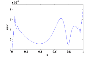
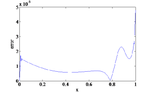
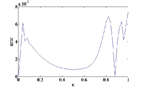
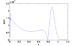
The absolute error distributions between the analytical and numerical solutions are drawn in Figs. 4-6 for various viscosity values and space steps. In these figures, the highest error appears about the right hand boundary position. We run the program again over the extended domain $\left[0,1.2\right]$ with parameters $\nu=0.005,$ $h=0.005$, the highest error is reduced at the right boundary seen in the Fig. 7 and $L_{\infty}$ error norm decrease from $4.790609\times 10^{-3}$ to $2.259598\times 10^{-3}$ at time $t=3.1$.

Figure 4:  Absolute error for $\nu=0.01\text{, }h=0.02\text{, }p=0.005111$

Figure 5:  Absolute error for $\nu=0.005\text{, }h=0.005\text{, }p=0.005941$

Figure 6:  Absolute error for $\nu=0.005\text{, }h=0.02\text{, }p=0.000739$

Figure 7:  Absolute error for $\nu=0.005\text{, }h=0.005\text{, }$$p=0.005941\text{ over }[0,1.2]$

(b) A well-known analytical solution of Burgers’ equation is

$$u(x,t)=\dfrac{\alpha+\mu+\left(\mu-\alpha\right)\exp\eta}{1+\exp\eta},\text{\quad}0\leq x\leq 1,\text{ }t\geq 0,$$ (18)

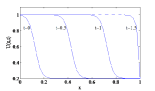
where $\eta=\dfrac{\alpha\left(x-\mu t-\gamma\right)}{\nu}$. $\alpha,$ $\mu$ and $\gamma$ are constants. Parameters $\alpha=0.4,$ $\mu=0.6$ and $\gamma=0.125$ are used to coincide with the some previous studies. This solution involves a travelling wave and move to the right with speed $\mu$. Initial condition is obtained from Eq. (18) when $t=0$. The boundary conditions are $u(0,t)=1,$ $u(1,t)=0.2$ for $t>0$.

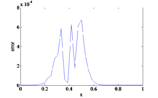
The calculation is performed with time step $\Delta t=0.01$, space step $h=1/36$ and viscosity coefficient $\nu=0.01$. The program is run up to time $t=0.5$. We have found $L_{\infty}=6.73543978\times 10^{-4}$ for the exponential B-spline Galerkin method at time $t=0.5$ documented in Table 3 with results of the quadratic B-spline Galerkin method [12], the quartic B-spline collocation method [16], the quintic B-spline collocation method [17] and the quartic B-spline Galerkin method [18].

The numerical solution obtained by the presented schemes gives better results than the others. The profiles of initial wave and solution at some times are depicted in Fig. 8. Error variations of the schemes are given in Fig. 9 at time $t=0.5$.

Figure 8:  Solutions for $\nu=0.01$

Figure 9:  Absolute error for $\nu=0.01$

Table 3: Comparison of results at $$t=0.5$$ for ,

Method

)

Ref.[12] (QBGM)

Ref.[16] (QBCM1)

Ref.[17] (QBCA1)

Ref.[18] (QBGM)

4 Conclusion

In this paper, we investigate the utility of the exponential B-spline in the Galerkin algorithm for solving the Burgers’ equation. The efficiency of the method is tested for a shock propagation solution and a travelling solution of the Burgers’ equation. For the first test problem, solutions found with the present methods are in good agreement with the results obtained by previous studies. In the second test problem, present method leads to accurate results than all of the others. In conclude, the numerical algorithm in which the exponential B-spline functions are used, performs well compared with other existing numerical methods for the solution of Burgers’ equation.

Acknowledgements: The authors are grateful to The Scientific and Technological Research Council of Turkey for financial support given for the project 113F394.

References

• [1] S.G. Rubin and R.A. Graves Jr., Viscous flow solutions with a cubic spline approximation, Computers & Fluids, 3 (1975), 1-36.
• [2] P.C. Jain and D.N. Holla, Numerical solution of coupled Burgers’ equation, International Journal of Non-Linear Mechanics, 13 (1978), 213-222.
• [3] A.M. Davies, Application of the Galerkin method to the solution of Burgers’ equation, Computer Methods in Applied Mechanics and Engineering, 14 (1978), 305-321.
• [4] B.J. McCartin, Theory computation and application of exponential splines, 1981, DOE/ER/03077-171.
• [5] B. J. McCartin, Computation of exponential splines, SIAM Journal on Scientific and Statistical Computing, 11 (1990), 242-262.
• [6] B. J. McCartin and A. Jameson, Numerical solution of nonlinear hyperbolic conservation laws using exponential splines, Computational Mechanics, 6 (1990), 77-91
• [7] B.J. McCartin, Theory of exponential splines, Journal of Approximation Theory, 66 (1991), 1-23.
• [8] A.H.A. Ali, L.R.T. Gardner and G.A. Gardner, A collocation method for Burgers’ equation using cubic splines, Computer Methods in Applied Mechanics and Engineering, 100 (1992), 325-37.
• [9] I. Dag, B. Saka and A. Boz, Quintic B-spline Galerkin Method for Numerical Solutions of the Burgers’ Equation, Dynamical Systems and Applications, Proceedings, 295-309, 2004, Antalya, Turkey.
• [10] S. Kutluay, A. Esen and I. Dag, Numerical solutions of the Burgers’ equation by the least squares quadratic B-spline finite element method, Journal of Computational and Applied Mathematics, 167 (2004), 21-33.
• [11] T. Ozis, A. Esen and S. Kutluay, Numerical solution of Burgers’ equation by quadratic B-spline finite elements, Applied Mathematics and Computation, 165 (2005), 237-249.
• [12] I. Dag, B. Saka and A. Boz, B-spline Galerkin methods for numerical solutions of the Burgers’ equation, Applied Mathematics and Computation, 166 (2005), 506-522.
• [13] I. Dag, D. Irk and A. Sahin, B-spline collocation methods for numerical solutions of the Burgers’ equation, Mathematical Problems in Engineering, 2005 (2005), 521-38.
• [14] M.A. Ramadan, T.S. El-Danaf, F.E.I. Abd Alaal, A numerical solution of the Burgers’ equation using septic B-splines, Chaos, Solitons and Fractals, 26 (2005),795-804.
• [15] I. Dag, D. Irk and B. Saka, A numerical solution of the Burgers’ equation using cubic B-splines, Applied Mathematics and Computation, 163 (2005), 199-211.
• [16] B. Saka and I. Dag, Quartic B-spline collocation methods to the numerical solutions of the Burgers’ equation, Chaos, Solitons and Fractals, 32 (2007), 1125-1137.
• [17] B. Saka and I. Dag, A numerical study of the Burgers’ equation, Journal of the Franklin Institute, 345 (2008), 328-348.
• [18] B. Saka and I. Dag, Quartic B-spline Galerkin approach to the numerical solution of the KdVB equation, Applied Mathematics and Computation, 215 (2009), 746-758.
• [19] C. Zhu and R. Wang, Numerical solution of Burgers’ equation by cubic B-spline quasi-interpolation, Applied Mathematics and Computation, 208 (2009), 260-272.
• [20] Z. Jiang and R. Wang, An Improved Numerical Solution of Burgers’ Equation by Cubic B-spline Quasi-interpolation, Journal of Information & Computational Science, 7 (2010),1013-1021.
• [21] I. Dag, A. Canivar, A. Sahin, Taylor–Galerkin and Taylor-collocation methods for the numerical solutions of Burgers’ equation using B-splines, Communications in Nonlinear Science and Numerical Simulation, 16 (2011), 2696-2708.
• [22] R.C. Mittal, R.K. Jain, Numerical solutions of nonlinear Burgers’ equation with modified cubic B-splines collocation method, Applied Mathematics and Computation, 218 (2012), 7839-7855.
• [23] H.V. Chapani, V.H. Pradhan and M.N. Mehta, Numerical simulation of Burgers’ equation using quadratic B-splines, International Journal of Applied Mathematics and Mechanics, 8 (2012), 18-32.
• [24] A. Korkmaz and I. Dag, Cubic B-spline differential quadrature methods and stability for Burgers’ equation, Engineering Computations, 30 (2013), 320-344, 2013.
• [25] G. Arora and B.K. Singh, Numerical solution of Burgers’ equation with modified cubic B-spline differential quadrature method, Applied Mathematics and Computation, 224 (2013), 166-177.
• [26] R. Mohammadi, Exponential B-spline solution of convection-diffusion equation, Applied Mathematics, 4 (2013), 933-944.
• [27] O. Ersoy and I. Dag, The exponential cubic B-spline algorithm for Korteweg-de Vries equation, Advances in Numerical Analysis, 2015 (2015).
• [28] I. Dag and O. Ersoy, Numerical solution of generalized Burgers-Fisher equation by exponential cubic Bspline collocation method, AIP Conference Proceedings 1648, 370008, 2015.