A semiparametric mixture method for local false discovery rate estimation

Abstract

We propose a semiparametric mixture model to estimate local false discovery rates in multiple testing problems. The two pilars of the proposed approach are Efron’s empirical null principle and log-concave density estimation for the alternative distribution. Compared to existing methods, our method can be easily extended to high dimension. Simulation results show that our method outperforms other existing methods and we illustrate its use via case studies in astronomy and microarray.

Keywords and Phrases: Brown-Stein model, false discovery rate, log-concave, mixture model, semiparametric model

1 Introduction

We consider a specialization of the Brown-Stein model used by Efron (2008a). Suppose that $(\delta_{1},Z_{1}),\ldots,(\delta_{N},Z_{N})$ are independently generated by the following hierarchical model:

$$\delta \sim g(\delta)=p_{0}g_{0}(\delta)+(1-p_{0})g_{1}(\delta)$$ (1)

$$Z|\delta \sim f(z|\delta)=\phi_{\delta,1}(z)$$ (2)

where $g_{0}(\delta)=\phi_{\mu,\sigma^{2}}(\delta)$ and $\phi_{\mu,\sigma^{2}}$ is the normal probability density function with mean $\mu$ and variance $\sigma^{2}$. Here we assume the probability $p_{0}$ and the probability density function $g_{1}$ are unknown.

The marginal distribution of $Z$ is given as follows:

$$f(z)=\int\phi(z-\delta)g(\delta)d\delta=p_{0}\phi_{\mu,\tau^{2}}(z)+(1-p_{0})f_{1}(z)$$

where $\phi(\cdot)=\phi_{0,1}(\cdot)$, $\tau^{2}=\sigma^{2}+1$ and $f_{1}(z)=\int\phi(z-\delta)g_{1}(\delta)d\delta$.

The model appears in three contexts: (i) in multiple testing problems (fMRI, microrarray), probit transformed $p$-values under $H_{0}$ follows the standard normal distribution while the mariganl probability density function of the probit transformed $p$-values associated with $H_{1}$ is unknown (Efron, 2008a); (ii) in variable/basis selection, a mixture prior is used to achieve sparsity (Johnstone and Silverman, 2005); (iii) in prediction, Fisher’s discriminant function can be regularized using a connection with the false discovery rate theory (Efron, 2008b). Due to close connections between the false discovery rate and all aforementioned problems, we will explain our model in the framework of multiple testing through this paper.

Suppose that we observe $N$ cases each with some effect size $\delta_{i}$ from either null ($\delta_{i}=0$) or alternative ($\delta_{i}\neq 0$) with the prior probability $p_{0}=\Pr\{\mbox{null}\}$ or $p_{1}=\Pr\{\mbox{alternative}\}=1-p_{0}$ and with $z$-values having density $f$:

$$f(z)=p_{0}f_{0}+(1-p_{0})f_{1}(z).$$

Here $Z$ can be either test statistics or probit-transformed $p$-values.

In multiple testing, adjusting for multiplicity is of great interest, To do so, we may consider to control for either the local false discovery rate, $fdr(z)=\Pr(\delta_{i}=0\mid z_{i})$ or the False Discovery Rate, $FDR(z)=\Pr(\delta_{i}=0\mid Z_{i}>z)$ assuming one-sided testing. In this paper, we focus on estimating $fdr(z)$ that can be viewed as the posterior probability of a case being from the null given $z$. Under the mixture model above, it is straightforward to show

$$fdr(z)=p_{0}f_{0}(z)/f(z).$$

It is natural to assume that $f_{0}$ follows the standard normal distribution. However, Efron (2008a) suggested that theoretical null distribution $N(0,1)$ may not be suitable for $f_{0}$ and proposed to estimate $f_{0}$ with the empirical null distribution $N(\mu,\tau^{2})$ where $\mu$ and $\tau$ are to be estimated from data. Furthermore, he used the zero assumption to estimate $\pi_{0}$ and employed Lindsey’s method to estimate the marginal density $f$. Note that his estimates may not follow the original mixture structure since the estimates are given from separate procedures. In other words, the mixture only used to define $fdr$, but not for making inference of $fdr$.

In this paper, we propose a semiparametric mixture model that cover a rich class of distributions for alternative and estimate $\pi_{0},f_{0},f_{1}$ simultaneously based on the proposed mixture model. Furthermore, our method can be easily extended to high dimension.

The remainder of the paper is organized as follows. Section 2 introduces log-concave densities and our semiprarametric mixture model. In Section 3, we present numerical studies to show that our method outperforms other existing methods. Section 4 presents case studies including estimating distributions of radial velocities in astronomy and ophthalmologic gene expression data analysis. Section 5 concludes this paper.

2 Semiparametric Mixture Model

2.1 Mixture model with smoothed log-concave

In this section, we propose a semiparametric mixture model for $f$. We assume that $g_{1}$ belongs to log-concave densities. The semiparametric mixture prior results in another semiparametric mixture distribution for marginal distribution of $z$.

It is reasonable to assume that the alternative distribution for $p$-values is log-concave and defined on $(0,\frac{1}{2})$. The following theorem justifies the choice of log-concave as an alternative distribution for profit transformed $p$-values.

Theorem 1.

Let $H(t)$ and $h(t)$ denote the cdf and pdf of the alternative distribution of $p\mbox{-value}=Pr(Z>z)$. Suppose that $h(t)$ is log-concave and continuous differentiable and $(0,\frac{1}{2})$. Define $Z=\Phi^{-1}(1-p)$, probit-transformed $p$-value. Then the pdf of $Z$ is log-concave under the alternative.

Proof.

By Theorem 1 in Bagnoli and Bergstrom (2005), $H(t)$ is also log-concave on $(0,\frac{1}{2})$. Let $F_{1}(z)$ denote cdf of the alternative distribution of $Z$. Then

$$F_{1}(z)={\sf Pr}(Z\leq z)={\sf Pr}(\Phi^{-1}(1-p)\leq z)={\sf Pr}(1-p\leq\Phi(z))=1-H(1-\Phi(z))$$

Therefore, the pdf of $z$ is given as follows:

$$f_{1}(z)=\frac{d}{dz}F_{1}(z)=h(1-\Phi(z))\phi(z).$$

Note that $\Phi(z)$ is convex on ${\mathbb{R}}^{-}$. Since $h$ is log-concave, $h(1-\Phi(z))$ is log-concave by Theorem 7 in Bagnoli and Bergstrom (2005). Furthermore, a product of log-concave functions is also log concave. Therefore $f_{1}(z)$ is log-concave. ∎

Advantages of the class of log-concave densities that is a subset of unimodal densities are well studied in Walther (2002, 2009). Walther (2002) showed the existence of the nonparametric MLE of a univariate log-concave density that can be computed via an efficient algorithm such as an active set algorithm and an iterative convex minorant algorithm (Dümbgen and Rufibach, 2011). However, the MLE may have sharp discontinuities at the boundary of its support as well as sharp kinks. To remedy this issues, Dümbgen and Rufibach (2009) introduce a smoothed log-concave $\tilde{f}_{1}$, given by

$$\tilde{f}_{1}(t)=\int\phi_{z,a^{2}}(t)\hat{f}_{1}(z)dz.$$

for some bandwidth $a>0$. Here $\hat{f}_{1}$ is the nonparametric MLE of $f$. Since it is convolution of two log-concave densities, the smoothed log-concave also belongs to the class of log-concave densties.

Let $\tilde{F}$ and $\hat{F}$ be the distribution functions of $\tilde{f}$ and $\hat{f}$ respectively. Since $\tilde{f}$ is convolution of $N(0,a^{2})$ and $\hat{f}$, it is easy to show

$${\rm Var}(\tilde{F})=a^{2}+{\rm Var}(\hat{F}).$$

Based on the above equation, Dümbgen and Rufibach (2009) suggest to choose the bandwidth

$$a=\sqrt{{\rm Var}(\hat{F})-{\rm Var}(\tilde{F})},$$

where

$${\rm Var}(\hat{F})=\frac{1}{N-1}\sum_{i=1}^{N}(z_{i}-\bar{z})^{2},\quad{\rm Var}(\tilde{F})=\int(z-\bar{z})^{2}\hat{f}(z)dz,$$

with $\bar{z}=\sum_{i=1}^{N}z_{i}/N$.

Hence, the proposed semiparametric estimator of $f$ is

$$\hat{p}_{0}\phi_{\hat{\mu},\hat{\tau}^{2}}(z)+(1-\hat{p}_{0})\tilde{f}_{1}(z).$$

2.2 EM Algorithm

It is natural to consider an EM-type algorithm to fit the proposed semiparametric model. To do so, we first define the likelihood function:

$$\ell(\mu,\tau^{2},z,\Delta) = \sum_{i=1}^{N}\left[\Delta_{i}\log\phi_{\mu,\tau^{2}}(z_{i})+(1-\Delta_{i})\log f_{1}(z_{i})\right]$$

$$+\sum_{i=1}^{N}\left[\Delta_{i}\log p_{0}+(1-\Delta_{i})\log(1-p_{0})\right]$$

where $\Delta$ is a latent variable indicating the group membership.

Following Chang and Walther (2007), we first run the EM algorithm for a Gaussian mixture to get initial values of $\mu$ and $\tau$. Then the EM algorithm for the proposed semiparametric model is given below:

1. E-step: compute the posterior probability:

   $$\gamma_{i}={\rm E}(\Delta_{i}|\mu,\tau^{2},z)=\frac{\hat{p}_{0}\phi_{\hat{\mu},\hat{\tau}^{2}}(z_{i})}{\hat{p}_{0}\phi_{\hat{\mu},\hat{\tau}^{2}}(z_{i})+(1-\hat{p}_{0})\tilde{f}_{1}(z_{i})}$$

2. M-step: compute the smoothed log-concave estimator $\tilde{f}_{1}$ based on $z_{i}$ with weights $\gamma_{i}$ and

   $$\hat{\mu}=\frac{\sum_{i=1}^{N}\gamma_{i}z_{i}}{\sum_{i=1}^{N}\gamma_{i}},\quad\hat{\tau}^{2}=\frac{\sum_{i=1}^{N}\gamma_{i}(z_{i}-\hat{\mu})^{2}}{\sum_{i=1}^{N}\gamma_{i}},\quad\hat{p}_{0}=\frac{1}{N}\sum_{i=1}^{N}\gamma_{i}.$$

To compute the smoothed log-concave MLE $\tilde{f}$ in M-step, R package logcondens (Dümbgen and Rufibach, 2011) is used.

2.3 Extension to Multivariate Cases

Suppose one observe multivariate statistics $\mathbf{Z}=(Z_{1},\ldots,Z_{k})$ and each statistic provides unique information for data. It is easy to extend the concept of the $fdr$ to high dimension:

$$fdr(\mathbf{Z})=p_{0}\frac{f_{0}(\mathbf{Z})}{f(\mathbf{Z})}$$

However, applying Efron’s method to multivariate is not straightforward. For example, Lindsey’s method is no longer valid to estimate the null distribution even for 2-dimension.

Ploner et al. (2006) proposed to extend the local fdr to 2-dimension to address the problem of gene expression data with small variance. Specifically, they computed 2 dimensional local fdr with $t$-test statistics and standard error estimates for each gene. They estimated $f_{0}$ with discrete smoothing of binomial data after binning the data. However, their method still requires a smoothing parameter and has an issue with boundary bias. On the other hand, our method is straightforward to extend to multivariate and is not involved in choosing a smoothing parameter.

Cule et al. (2010) extended Dümbgen and Rufibach (2009) to multivariate settings and implemented multivariate smoothed log-concave estimation in R package logConcDEAD (Cule et al., 2009).

3 Simulation Studies

In this section we investigate the performance of the proposed semiparametric approach with simulation studies where we can compare the results with Efron’s method. We conduct $M=500$ Monte Carlo experiments with the sample size $N=1,000$ and use three measures of performance: empirical False Discovery Rate (FDR), empirical False Nondiscovery Rate (FNR) and the Root Mean Squared Error (RMSE) which is given by

$${\rm RMSE}=\frac{1}{M}\sum_{r=1}^{M}\sqrt{{\sum_{i:{\rm fdr}(z_{i}^{()r})\leq 0.5}\left\{\widehat{\rm fdr}(z_{i}^{(r)})-{\rm fdr}(z_{i}^{(r)})\right\}^{2}}\left/{\sum_{i=1}^{N}I({\rm fdr}(z_{i}^{(r)})\leq 0.5)}\right.}.$$

where $z_{1}^{(r)},z_{2}^{(r)},\cdots,z_{N}^{(r)}$ is the $r$-th random sample generated from the Monte Carlo simulation. Here, we only consider ${\rm fdr}(z_{i}^{(r)})\leq 0.5$ in the definition of the RMSE because the accuracy of $fdr$ estimation is required mainly for the region where the $fdr$ is small. For example, we are usually interested in the behavior of $fdr$ estimates where ${\rm fdr}(z)\leq 0.2$.

Table 1: Simulation scenarios: $*$ indicates the convolution of two densities. ${\rm Gamma}_{2}(\alpha,\beta)$ denotes the bivariate gamma distribution of $(V_{1},V_{2})\stackrel{{\scriptstyle iid}}{{\sim}}{\rm Gamma(\alpha,\beta)}$.

Scenario			$p_{0}$		$f_{0}$		$f_{1}$
Univariate	1		0.95		$N(0,1)*N(0,10^{-6})$		$N(0,1)*N(3.5,0.5)$
	2		0.90		$N(0,1)*N(0,10^{-6})$		$N(0,1)*N(3.5,0.5)$
	3		0.80		$N(0,1)*N(0,10^{-6})$		$N(0,1)*N(3.5,0.5)$
	4		0.95		$N(0,1)*N(0,10^{-6})$		$N(0,1)*{\rm Gamma}(12,0.25)$
	5		0.90		$N(0,1)*N(0,10^{-6})$		$N(0,1)*{\rm Gamma}(12,0.25)$
	6		0.80		$N(0,1)*N(0,10^{-6})$		$N(0,1)*{\rm Gamma}(12,0.25)$
Bivariate	1		0.95		$N(\mathbf{0}_{2},\Sigma)*N(\mathbf{0}_{2},10^{-6}I_{2})$		$N(\mathbf{0}_{2},\Sigma)*N((3.5,3.5)^{\prime},0.5I_{2})$
	2		0.90		$N(\mathbf{0}_{2},\Sigma)*N(\mathbf{0}_{2},10^{-6}I_{2})$		$N(\mathbf{0}_{2},\Sigma)*N((3.5,3.5)^{\prime},0.5I_{2})$
	3		0.80		$N(\mathbf{0}_{2},\Sigma)*N(\mathbf{0}_{2},10^{-6}I_{2})$		$N(\mathbf{0}_{2},\Sigma)*N((3.5,3.5)^{\prime},0.5I_{2})$
	4		0.95		$N(\mathbf{0}_{2},\Sigma)*N(\mathbf{0}_{2},10^{-6}I_{2})$		$N(\mathbf{0}_{2},\Sigma)*{\rm Gamma}_{2}(12,0.25)$
	5		0.90		$N(\mathbf{0}_{2},\Sigma)*N(\mathbf{0}_{2},10^{-6}I_{2})$		$N(\mathbf{0}_{2},\Sigma)*{\rm Gamma}_{2}(12,0.25)$
	6		0.80		$N(\mathbf{0}_{2},\Sigma)*N(\mathbf{0}_{2},10^{-6}I_{2})$		$N(\mathbf{0}_{2},\Sigma)*{\rm Gamma}_{2}(12,0.25)$

3.1 Simulations for univariate models

We consider 6 scenarios for simulations. For the first 3 scenarios, we assume normal mixtures for null and alternative distributions with different $p_{0}$. The next 3 scenarios are the same as the first 3 except using a log-concave distribution as an alternative.

Tables 2 and 3 summarize the simulation results. Table 2 shows that the proposed approach stably yields good $p_{0}$ estimates for a wide range of target values while Efron’s method tends to give overestimates $p_{0}$ especially when $p_{0}$ is relatively small. When the alternative follows a log-concave, the performance of our method are similar to that with a normal alternative. However, Efron method is slightly worse with the log-concave alternative. As a result, multiple testing procedure with Efron’s method becomes too conservative when $p_{0}$ is small. Table 3 reports similar results. The RMSEs of Efron’s method increase as $p_{0}$ decreases and are worse with the log-concave alternative.

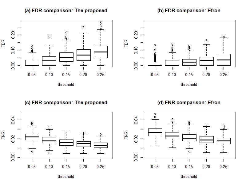
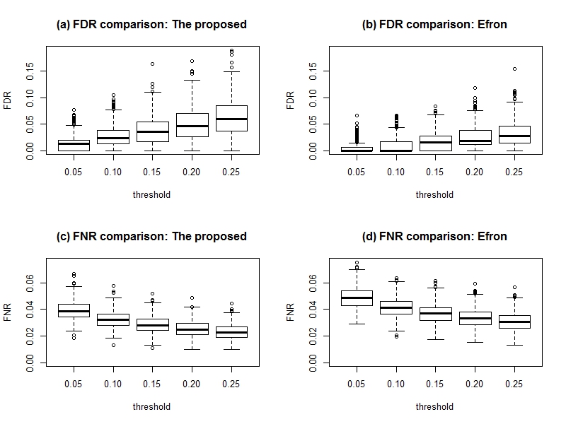
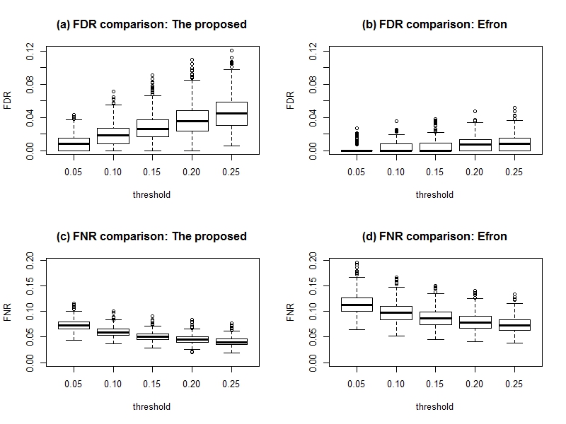
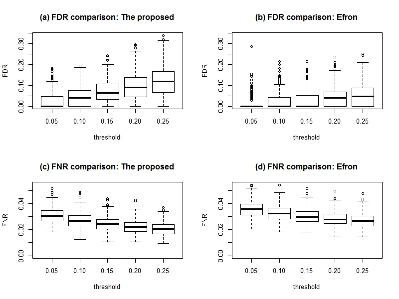
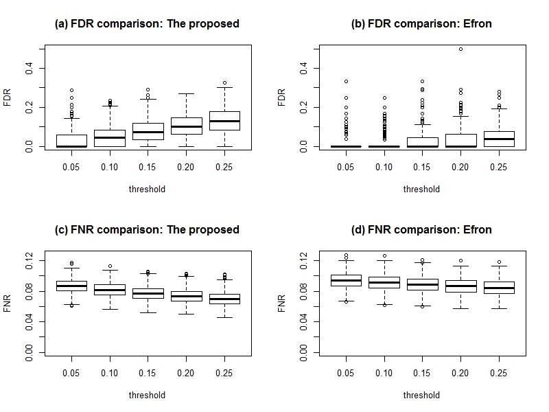
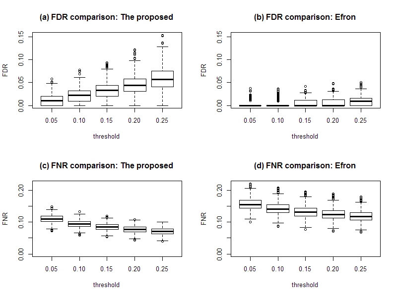
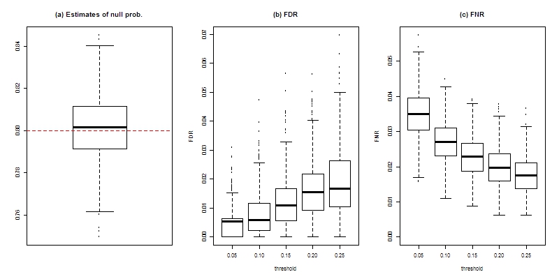
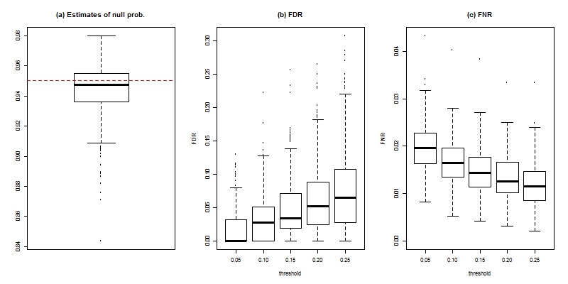
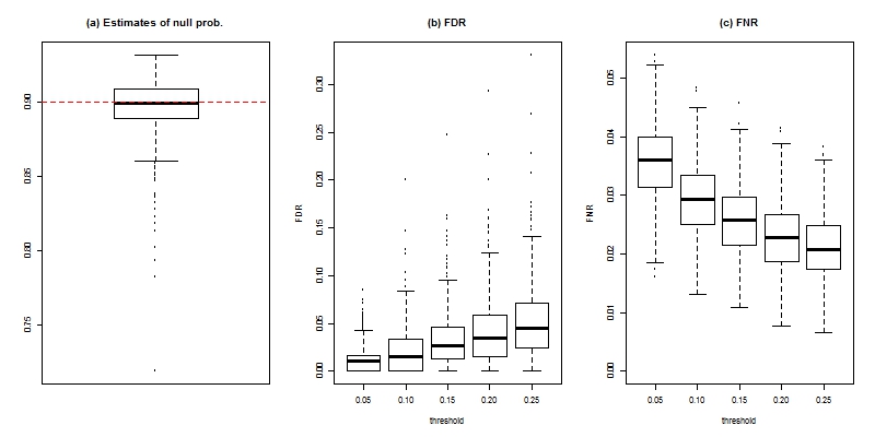
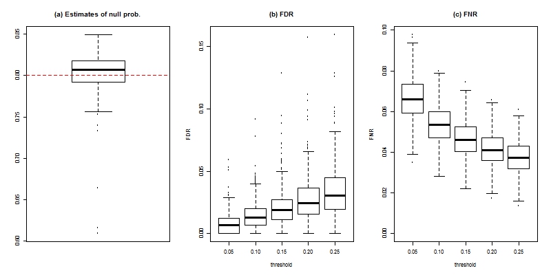
Figure 1 illustrates the comparisons of the three performance measures in Scenario 1 with various $fdr$ levels (from 0.05 to 0.25). Efron’s method reports low FDR values regardless of $fdr$ values at the cost of higher FNR values. While there is no clear relationship between $fdr$ and FDR, Efron (2007) indicated $fdr=0.20$ corresponds to FDR values between 0.05 and 0.15. Hence our method seems to control the FDR reasonably well given $fdr$ levels with lower FNR values. Similar patterns are founds in Figures 2 - 6 for other scenarios.

Table 2: Summary of $p_{0}$ estimation results from univariate models

			Proposed			Efron
Scenario	$p_{0}$		Mean	standard error		Mean	standard error
1	0.95		0.9293	0.0006		0.9490	0.0021
2	0.90		0.8840	0.0006		0.8971	0.0017
3	0.80		0.7910	0.0007		0.8878	0.0027
4	0.95		0.9316	0.0006		0.9577	0.0022
5	0.90		0.8915	0.0006		0.9169	0.0017
6	0.80		0.8057	0.0008		0.9215	0.0024

Table 3: RMSE comparison of $fdr$ estimates for univariate models

		Proposed			Efron
Scenario		Mean	standard error		Mean	standard error
1		0.1059	0.0017		0.0728	0.0026
2		0.0807	0.0015		0.0712	0.0025
3		0.0581	0.0013		0.2520	0.0044
4		0.1074	0.0018		0.0891	0.0033
5		0.0754	0.0016		0.1185	0.0033
6		0.0456	0.0013		0.3730	0.0039

Figure 1: Empirical False Discovery Rate and empirical False Nondiscovery Rate from the proposed method and Efron’s method for Scenario 1 in the univariate simulations. The threshold are $fdr$ values. The boxplots are drawn with the values resulted from $M=500$ Monte Carlo simulations.

Figure 2: Empirical False Discovery Rate and empirical False Nondiscovery Rate from the proposed method and Efron’s method for Scenario 2 in the univariate simulations. The threshold are $fdr$ values. The boxplots are drawn with the values resulted from $M=500$ Monte Carlo simulations.

Figure 3: Empirical False Discovery Rate and empirical False Nondiscovery Rate from the proposed method and Efron’s method for Scenario 3 in the univariate simulations. The threshold are $fdr$ values. The boxplots are drawn with the values resulted from $M=500$ Monte Carlo simulations.

Figure 4: Empirical False Discovery Rate and empirical False Nondiscovery Rate from the proposed method and Efron’s method for Scenario 4 in the univariate simulations. The threshold are $fdr$ values. The boxplots are drawn with the values resulted from $M=500$ Monte Carlo simulations.

Figure 5: Empirical False Discovery Rate and empirical False Nondiscovery Rate from the proposed method and Efron’s method for Scenario 5 in the univariate simulations. The threshold are $fdr$ values. The boxplots are drawn with the values resulted from $M=500$ Monte Carlo simulations.

Figure 6: Empirical False Discovery Rate and empirical False Nondiscovery Rate from the proposed method and Efron’s method for Scenario 1 in the univariate simulations. The threshold are $fdr$ values. The boxplots are drawn with the values resulted from $M=500$ Monte Carlo simulations.

3.2 Simulations for bivariate models

We consider similar scenarios for bivariate models. Define

$$\mathbf{0}_{2}=\begin{pmatrix}0\\ 0\end{pmatrix},\quad\mathbf{1}_{2}=\begin{pmatrix}1\\ 1\end{pmatrix},\quad I_{2}=\begin{pmatrix}1&0\\ 0&1\end{pmatrix},\quad\Sigma=\begin{pmatrix}1&0.3\\ 0.3&1\end{pmatrix}.$$

The simulation scenarios are similar to those of univariate cases. In each scenario, the marginal distributions of null and alternative are the same as the null and alternative distributions of the corresponding scenario in univariate models. By doing so, we want to find whether there is any advantage of 2-dimensional $fdr$ compared to 1-dimensional $fdr$. Like

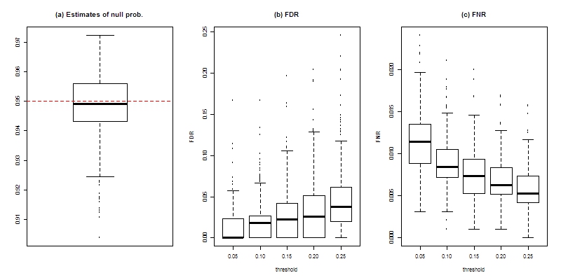
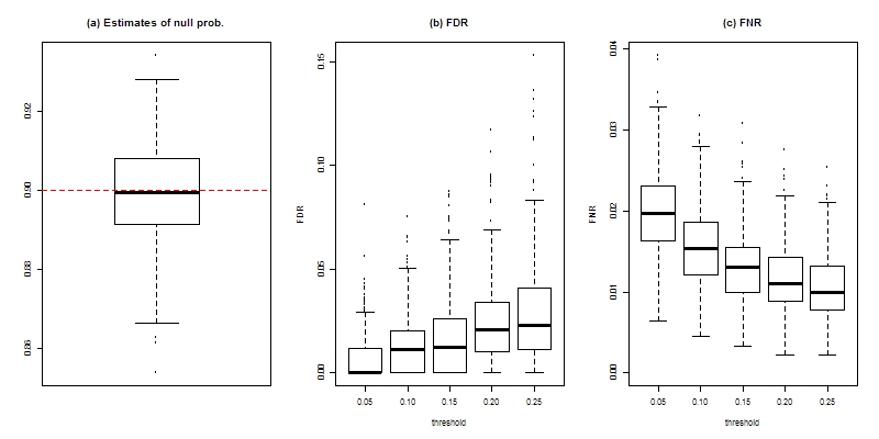
Figure 7 – Figure 12 present the distributions of the $p_{0}$ estimates, empirical FDR and empirical FNR with various $fdr$ levels for each scenario. All the figures show that the proposed method works reasonably well. It is interesting to observe that the performance of the proposed method in bivariate models looks better than in univariate setting. Comparing the boxplots of FDR and FNR in panel (b) and (c) of the figures with those in the panels (b) and (c) of Figure 1 – Figure 6, we confirm that empirical FDR and FNR in the bivariate models are lower than those from the corresponding univariate models. Bivariate method could do better by taking account of extra information since it allows the test procedure an additional flexibility in deciding the boundary of the rejection region.

Figure 7: (a) $p_{0}$ estimates, (b) empirical FDR, (c) empirical FNR for Scenario 1 in the bivariate models with $p_{0}=0.95$ and $f_{1}$ = Normal*Normal.

Figure 8: (a) $p_{0}$ estimates, (b) empirical FDR, (c) empirical FNR for Scenario 2 in the bivariate models with $p_{0}=0.90$ and $f_{1}$ = Normal*Normal.

Figure 9: (a) $p_{0}$ estimates, (b) empirical FDR, (c) empirical FNR for Scenario 2 in the bivariate models with $p_{0}=0.80$ and $f_{1}$= Normal*Normal.

Figure 10: (a) $p_{0}$ estimates, (b) empirical FDR, (c) empirical FNR for Scenario 2 in the bivariate models with T $p_{0}=0.95$ and $f_{1}$= Normal*Gamma.

Figure 11: (a) $p_{0}$ estimates, (b) empirical FDR, (c) empirical FNR for Scenario 2 in the bivariate models with $p_{0}=0.90$ and $f_{1}$= Normal*Gamma.

Figure 12: (a) $p_{0}$ estimates, (b) empirical FDR, (c) empirical FNR for Scenario 2 in the bivariate models with $p_{0}=0.80$ and $f_{1}$= Normal*Gamma.

4 Case Studies

4.1 Ophthalmologic gene expression data analysis

In this subsection, we consider an Affymetrix data set with a paired design (Smith et al., 2007; Choi et al., 2008). Donor-matched retina and choroidal endothelial cells from three human cadavers were treated with Toxoplasma gondii tachyzoite or medium alone. We are interested in treatment effects. It measured gene expression levels in retina and choroid. Two tissues are next to each other, yet quite unique. Gene expression profiling experiment were performed by Affymetrix Human Genome Focus array that contains 8746 human gene transcripts. More details on experiment and normalization can be found in Smith et al. (2007).

Let $y_{ij}$ be $j$th gene expression value of $i$th subject. A simple linear model is fitted to the normalized data to find out significantly changed genes in each cell type.

Model 1 (retina): $$y_{ij}=\beta_{0}+\beta_{t}\cdot\mbox{treatment}+\beta_{i}\cdot\mbox{subject}_{i}+\epsilon_{ij},$$

Model 2 (choroid): $$y_{ij}=\beta_{0}+\beta_{t}\cdot\mbox{treatment}+\beta_{i}\cdot\mbox{subject}_{i}+\epsilon_{ij}.$$

An empirical Bayes implemented in R package limma (Ritchie et al., 2015) is used to fit the models to the normalized data. With 1-D $fdr<0.05$, there are 248 and 173 significantly changed probe sets for the treatment group in Model 1 and 2, respectively. There are 68 common probe sets detected by both models and in total 353 probe sets are detected by at least one of them. In comparison, when applying the proposed 2-D $fdr$, there are 713 significant probe sets with 2-D $fdr<0.05$. The proposed 2-D $fdr$ could detect more than twice of probe sets that are detected by 1-D $fdr$ applied separately.

For comparison, another linear model that is more likely used in practice for the study is fitted with 1-D $fdr$. Now let $y_{ijk}$ be the $j$th gene expression level of $i$th subject in $k$th cell type.

$$\mbox{Model 3 :}y_{ijk}=\beta_{0}+\beta_{t}\cdot\mbox{treatment}+\beta_{i}\cdot\mbox{subject}_{i}+\beta_{c}\cdot\mbox{cell type}+\epsilon_{ijk}$$

Four hundred one probe sets had $fdr<0.05$ less than 0.05, which is somewhat closer to 353 significant probe sets detected by 1-D $fdr$ apply to each cell type separately. When crosstabulated with 713 significant probe sets based 2-D $fdr$, there are 164 common probe sets between the two approaches.

A gene ontology analyses are performed by NIH DAVID (Database for Annotation, Visualization and Integrated Discovrey) to compare 713 significant probe sets based on 2-D $fdr$ to 401 based on 1-D $fdr$ of model 3. The former list returned 108 chart records of functional annotation with $fdr<0.05$. Interestingly, the analysis also detects that the list is abundant with genes from eye ($p=0.020$) and t-cell ($p=0.047$). In comparison, similar analyses of the latter list of 401 probe sets returns only 85 significant chart records and $p$-values for abundance of genes in eye or t-cell are not significant (0.113 or 0.075, respectively).

4.2 Radial velocity distribution in astronomy

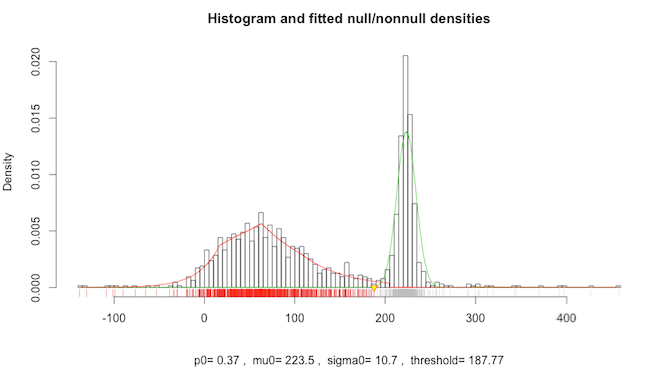
The radial velocity of a star play a key role in detecting exoplanet and is of great interest in astronomy (Fabrizio et al., 2011). The data are radial velocity measurements of 1266 luminous stars mainly from the Carina, a dwarf spheroidal galaxy and a companion of the Milky Way (Patra and Sen, 2016). Some of data are also from the Milky Way. Astronomers are interested in estimating the distribution of radial velocities that is believed to be a two-component mixture where one is a Gaussian and the other is a non-Gaussian. We are particularly interested in understanding the Gaussian component of the Radial Velocity distribution.

This data set was analyzed by Patra and Sen (2016). They reported that the estimate of $p_{0}$=0.36 and the estimated location of the peak (=$\mu_{0}$) is 229.1 with the estimated stand deviation is 7.51. Figure 13 shows the mixture of two components estimated by the proposed method. The right one is considered as the Gaussian part (Fabrizio et al., 2011). Our method presents $\hat{p}_{0}=0.37$, $\hat{\mu}_{0}=223.5$ and $\hat{\sigma}_{0}=10.7$. With slightly different data sets, Fabrizio et al. (2011) reported the peaks around 220.4-221.4 with the standard deviation 8.0-11.7.

Figure 13: Density of the Redial Velocity Distribution

5 Conclusion

In this paper we proposed a semiparametric two component mixture model based on normal and log concave densities. Our method is flexible because it does not require smoothing parameter selection and the log-concavity assumption of the alternative is reasonable. We discuss the connection between the proposed model and multiple testing. Our method estimate $fdr$ and the proportion of the null simultaneously and fit the alternative when necessary.

We presented an EM-type algorithm to implement the proposed estimators and can be easily extended to multivariate settings. Our simulation studies suggested that the proposed method outperforms other existing method in both univariate and bivariate settings. We present two case studies which shows the flexibility of the semiparametric mixture model in estimating Radial Velocity distributions in astronomy and advantages of using 2-d $fdr$ over 1-d $fdr$ in microarray.

In general, semiparametric mixture models are nonidentifiable without additional assumptions on $f_{1}$. Assuming that $f_{1}$ belongs to the location-shift family of distributions, Bordes et al. (2006) showed the identifiability of the semiparametric mixture model under mild regularity conditions. Genovese and Wasserman (2004) also addressed identifiability for mixture models for $p$-value distribution under the assumption that the null is uniform. We left the identifiability of our mixture model as a future work.

References

- Bagnoli and Bergstrom (2005) Bagnoli and Bergstrom (2005). Log-concave probability and its applications. Economic Theory 26 445–469.
- Bordes et al. (2006) Bordes, L., Delmas, C., and Vandekerkhove, P. (2006). Semiparametric estimation of a two-component mixture model where one component is known. Scandinavian Journal of Statistics 33 733–752.
- Chang and Walther (2007) Chang, G. T. and Walter, G. (2007). Clustering with mixtures of log-concave distributions. Computational Statistics and Data Analysis 51 6242–6251.
- Choi et al. (2008) Choi, D., Appukuttan, B., Binek, S. J., Planck, S. R., Stout, J. T., Rosenbaum, J. T. and Smith, J. R. (2008). Prediction of Cis-Regulatory elements controlling genes differentially expressed by retinal and choroidal vascular endothelial. Journal of Ocular Biology, Diseases and Informatics. 1, 37-45.
- Cule et al. (2009) Cule, M., Gramacy, R. and Samworth, R. (2009). LogConcDEAD: An R package for maximum likelihood estimation of a multivariate log-concave density. Journal of Statistical Software 29 Issue 2.
- Cule et al. (2010) Cule, M., Samworth, R. and Stewart, M. (2010). Maximum likelihood estimation of a multi-dimensional log-concave density. Journal of the Royal Statistical Society: Series B 72 545–607.
- Dümbgen and Rufibach (2009) Dümbgen, L. and Rufibach, K. (2009). Maximum likelihood estimation of a log-concave density and its distribution function: basic properties and uniform consistency. Bernoulli 15 40–68.
- Dümbgen and Rufibach (2011) Dümbgen, L. and Rufibach, K. (2011). logcondens: Computations related to univariate log-concave density estimation. Journal of Statistical Software 39 1–28.
- Efron (2007) Efron, B. (2007). Size, power and false discovery rates. Annals of Statistics 35 1351–1377.
- Efron (2008a) Efron, B. (2008a). Microarray, empirical Bayes and the two-groups model. Statistical Sciences 23 1–22.
- Efron (2008b) Efron, B. (2008b). Empirical Bayes Estimates for Large-Scale Prediction Problems. Journal of the American Statistical Assocation 104 1015–1028.
- Fabrizio et al. (2011) Fabrizio, M., Nonino, M., Bono, G., Ferraro, I., François, P., Iannicola, G., Monelli, M., Thévenin, F., Stetson, P. B., Walker, A. R., Buonanno, R., Caputo, F., Corsi, C. E., Dall’Ora, M., Gilmozzi, R., James, C. R., Merle, T., Pulone, L. and Romaniello, M. (2011). The Carina Project. IV. Radial Velocity Distribution. Publications of the Astronomical Society of the Pacific 123 384–401.
- Genovese and Wasserman (2004) Genovese, C. and Wasserman, L. (2004). A stochastic process approach to false discovery control. Annals of Statistics 32 1035–1061.
- Johnstone and Silverman (2005) Johnstone, I. M. and Silverman, B. W. (2005). Empirical Bayes selection of wavelet thresholds. Annals of Statistics 33 1700–1752.
- Patra and Sen (2016) Patra, R. K. and Sen, B. (2016). Estimation of a two-component mixture model with applications to multiple testing. Journal of the Royal Statistical Society, Series B, To appear.
- Ploner et al. (2006) Ploner, A., Calza, S., Gusnanto, A. and Pawitan, Y. (2006). Multidimensional local false discovery rate for microarray studies. Bioinformatics 22 556–565.
- Ritchie et al. (2015) Ritchie. M. E., Phipson, B., Wu, D., Hu, Y., Law, C. W., Shi, W. and Smyth, G. K. (2015). limma powers differential expression analyses for RNA-sequencing and microarray studies. Nucleic Acids Research 43 e47.
- Robin et al (2007) Robin, S., Bar-Hen, A., Daudin, J.J. and Pierre, L. (2007). A semi-parametric approach for mixture models: Application to local false discovery rate estimation.
- Smith et al. (2007) Smith, J. R., Choi, D., Chipps, T., Pan, Y., Zamora, D., Babra, B., Davies, M., Planck, S. R. and Rosenbaum, J. T. (2007). Unique gene profiles of human retinal and choroidal vascular endothelium in donor-matched cell cultures. Investigative Ophthalmology and Vision Sciences. 48 2676–2684.
- Walther (2002) Walther, G. (2002). Detecting the presence of mixing with multiscale maximum likelihood. Journal of the American Statistical Association 97 508–513.
- Walther (2009) Walther, G. (2009). Inference and modeling with log-concave distributions. Statistical Science 24 319–327.