Hall Response and Edge Current Dynamics in Chern Insulators out of Equilibrium

Abstract

We investigate the transport properties of Chern insulators following a quantum quench between topological and non-topological phases. Recent works have shown that this yields an excited state for which the Chern number is preserved under unitary evolution. However, this does not imply the preservation of other physical observables, as we stressed in our previous work. Here we provide an analysis of the Hall response following a quantum quench in an isolated system, with explicit results for the Haldane model. We show that the Hall conductance is no longer related to the Chern number in the post-quench state, in agreement with previous work. We also examine the dynamics of the edge currents in finite-size systems with open boundary conditions along one direction. We show that the late-time behavior is captured by a Generalized Gibbs Ensemble, after multiple traversals of the sample. We discuss the effects of generic open boundary conditions and confinement potentials.

I Introduction

Topological states of matter exhibit a wealth of novel properties due to their extreme resilience to local perturbations. A striking manifestation is the quantum Hall effect Klitzing et al. (1980), where the exact quantization of the Hall response is immune to sample defects Laughlin (1981). This robustness is intimately linked to the topological Chern invariant, which has direct signatures in quantum transport Thouless et al. (1982); Niu et al. (1985). Recent theory and experiments have exposed many new examples of topological phenomena, including the relativistic quantum Hall effect in graphene Murthy and Shankar (2003); Novoselov et al. (2005); Zhang et al. (2005), topological insulators Kane and Mele (2004); Bernevig et al. (2006); König et al. (2007); Khanikaev et al. (2013), and Majorana edge modes Fu and Kane (2008). Work has also focused on the generation of topological Floquet states through time-dependent driving Kitagawa et al. (2010); Lindner et al. (2011); Rechtsman et al. (2013).

Out of equilibrium, much less is known about the behavior of topological states. Early works on $p+ip$ superfluids have shown that topological invariants can be preserved following quenches of the interaction strength Foster et al. (2013, 2014). In the context of Chern insulators, recent studies have shown that the Chern number is robust under unitary evolution, even following quenches between topological and non-topological phases D’Alessio and Rigol (2015); Caio et al. (2015). However, as we stressed in Ref. Caio et al. (2015), this does not imply the persistence of all physical observables. The presence or absence of edge states for example, depends on the final Hamiltonian and not just the initial state. In a similar way, the Hall response does not necessarily remain quantized. This is consistent with recent calculations by Wang et al Wang and Kehrein (2015); Wang et al. (2016), who have investigated the Hall response following a quantum quench, including an external reservoir to induce decoherence and reduce to the diagonal ensemble.

In this manuscript we examine the Hall response following a quantum quench in a completely isolated system undergoing unitary evolution. We focus on the Haldane model Haldane (1988), as recently realized using cold atomic gases Jotzu et al. (2014). We show that the Hall response is no longer quantized following a quantum quench between the topological and non-topological phases, in spite of the preservation of the Chern index in infinite-size samples. In the zero frequency limit our results agree with those of Refs Wang and Kehrein (2015); Wang et al. (2016), as oscillatory off-diagonal contributions vanish. The results are in good agreement with analytical approximations based on the low-energy Dirac Hamiltonian. We further examine the detailed properties of the edge currents following a quantum quench in finite-size systems. We show that the late-time behavior following many traversals of the sample is quantitatively described by a Generalized Gibbs Ensemble (GGE) Rigol et al. (2007, 2008); Caux and Konik (2012). With a view towards cold atom experiments we also consider the effects of harmonic confinement potentials.

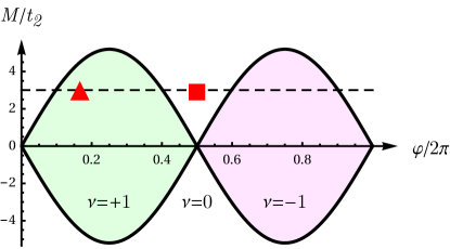
Figure 1: Phase diagram of the Haldane model showing topological ($\nu=\pm 1$) and non-topological phases ($\nu=0$) Haldane (1988). The triangle and the square indicate the starting points of quenches along the dashed line, as shown in Figs 4 and 5.

II Model

The Haldane model describes spinless fermions hopping on a honeycomb lattice with a staggered magnetic field Haldane (1988). The Hamiltonian is given by

$$\hat{H} = -t_{1}\sum_{\langle i,j\rangle}\left(\hat{c}^{{\dagger}}_{i}\hat{c}^{\mathstrut}_{j}+\mbox{h.c.}\right)-t_{2}\sum_{\langle\!\langle i,j\rangle\!\rangle}\left(e^{\mathrm{i}\varphi_{ij}}\hat{c}^{{\dagger}}_{i}\hat{c}^{\mathstrut}_{j}+\mbox{h.c.}\right)$$ (1)

$$+M\sum_{i\in A}\hat{n}_{i}-M\sum_{i\in B}\hat{n}_{i},$$

where $\hat{c}_{j}^{\dagger}$ and $\hat{c}_{j}$ are fermionic creation and annihilation operators obeying anti-commutation relations $\{\hat{c}_{j},\hat{c}_{j}^{\dagger}\}=\delta_{ij}$, and $\hat{n}_{i}\equiv\hat{c}_{i}^{\dagger}{\hat{c}_{i}}$. Here, $\langle i,j\rangle$ and $\langle\!\langle i,j\rangle\!\rangle$ indicate summation over the nearest and next-to-nearest neighbor sites respectively, $t_{1}$ and $t_{2}$ are the associated hopping parameters, and $A$ and $B$ label the two sublattices. The phase $\varphi_{ij}=\pm\varphi$ corresponds to the Aharonov-Bohm phase due to the staggered magnetic field and is taken positive (negative) in the anti-clockwise (clockwise) hopping direction. The associated time-reversal symmetry breaking leads to a quantum Hall effect, in the absence of a net magnetic field. The energy offset $M$ corresponds to spatial inversion symmetry breaking, allowing both non-topological and topological phases to be explored. The phase diagram of the Haldane model is shown in Fig. 1, where we assume that $|t_{2}/t_{1}|\leq 1/3$ so that the bands may touch, but not overlap Haldane (1988); see Fig. 2.

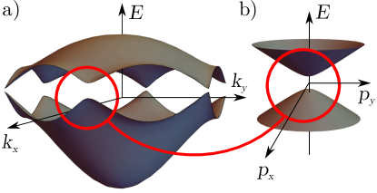
Figure 2: (a) Band structure of the Haldane model Haldane (1988). (b) At low-energies, the model reduces to a sum of two Dirac Hamiltonians with a gapped relativistic dispersion relation.

The topological and non-topological phases are distinguished by the Chern index $\nu$ Chern (1946); Thouless et al. (1982); Berry (1984); Haldane (1988) which takes the values $\nu=\pm 1$ and $\nu=0$ respectively. This is given by

$$\nu=\frac{1}{2\pi}\int d^{2}k\,\Omega,$$ (2)

where $\Omega=\partial_{k_{x}}A_{k_{y}}-\partial_{k_{y}}A_{k_{x}}$ is the Berry curvature, $A_{k_{\mu}}=i\Braket{\psi}{\partial_{k_{\mu}}}{\psi}$ is the Berry connection and the integral is performed over the first Brillouin zone. The boundaries of the topological phases correspond to $M/t_{2}=\pm 3\sqrt{3}\sin\varphi$, and are independent of $t_{1}$; see Fig. 1. In the remainder of the manuscript we choose $t_{2}=t_{1}/3$ and set $t_{1}=1$ such that $M$ is expressed in units of $t_{1}$. We also set the intersite spacing $a$ to unity.

III Quantum Quenches

As in Ref. Caio et al. (2015), we study quantum quenches between different points of the phase diagram shown in Fig. 1. We start from the ground state of $\hat{H}$ with parameters $(M_{0},\varphi_{0})$, and abruptly change them to new values $(M,\varphi)$. The system evolves unitarily under the new Hamiltonian, leading to a time-dependent state $\Ket{\psi(t)}=\exp\left[-i\hat{H}(M,\varphi)t/\hbar\right]\Ket{\psi_{0}}$. Here, $\Ket{\psi_{0}}$ is the initial ground state, corresponding to a band insulator of the half-filled system at $(M_{0},\varphi_{0})$. As shown in Refs D’Alessio and Rigol (2015); Caio et al. (2015), the corresponding Chern number remains unchanged from its initial value, even when quenching between different phases. Nonetheless, other observables may change. In finite-size systems, the topological and non-topological phases are distinguished by the presence or absence of edge states. The re-population of these states following a quantum quench leads to changes in the edge currents and the orbital magnetization  Caio et al. (2015). This is accompanied by the light-cone spreading of currents into the interior of the sample, and the onset of finite-size effects. It is evident that, for a finite-size system, the concept of a Chern index must eventually break down at late times following a quantum quench, as one cannot resolve momenta on scales smaller than the inverse system size, $L^{-1}$ . The Berry phase acquired upon circulating a plaquette of size $2\pi/L$ becomes ill-defined once the Berry connection $A_{k_{\mu}}$ becomes as large as $|A_{k_{\mu}}|\sim L$, and so too does the Chern number. Since, out of equilibrium, $|\psi\rangle$ is in a superposition of ground and excited states, it oscillates at the energy difference $\Delta E_{\bm{k}}$. The associated Berry connection $A_{k_{\mu}}=\langle\psi(t)|\partial_{k_{\mu}}|\psi(t)\rangle$ grows in time, $t$, as $A_{k_{\mu}}\sim[\partial\Delta E_{\bm{k}}/\partial(\hbar k)_{\mu}]t=vt$ where $v=\partial\Delta E_{\bm{k}}/\partial(\hbar k_{\mu})$ is a characteristic difference of band velocities, limited by $v\lesssim 2c$ with $c$ the maximum group velocity. Thus $|A_{k_{\mu}}|\sim L$ when $vt\sim L$, that is the Chern number becomes ill-defined for timescales larger than the time required for light-cone propagation across the interior of the sample, $t\gtrsim L/2c$.

IV Hall Response

In order to further differentiate the physical characteristics of the initial and final states, we examine the Hall response following a quantum quench. We apply a time-dependent electric field ${\bf E}(t)={\bf E}_{0}\cos\omega t$ and calculate the in-phase transverse response. In the presence of periodic boundary conditions it is convenient to generate this electric field by means of an auxiliary magnetic flux threading a toroidal sample Laughlin (1981); Thouless et al. (1982); Niu et al. (1985); see Fig. 3.

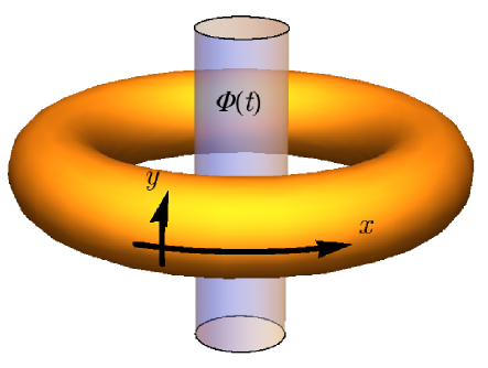
Figure 3: Setup used to evaluate the Hall response in the presence of periodic boundary conditions. An auxiliary time-dependent magnetic flux $\Phi(t)$ generates a longitudinal electric field $E_{x}(t)=-\frac{\partial\Phi(t)}{\partial t}$. Note that this flux does not correspond to the time-reversal symmetry breaking parameter $\varphi$ in the Haldane model. The Hall conductance $\sigma_{xy}(t)$ is obtained from the transverse current that is in phase with $E_{x}(t)$.

For recent work examining the dynamics of one-dimensional currents following “flux quenches” in ring geometries see Ref. Nakagawa et al. (2016).

In momentum space, the resulting Hamiltonian may be decomposed into a sum over independent modes $\hat{H}=\sum_{\bf k}\hat{H}_{\bf k}$ where $\hbar\dot{\bf k}=q{\bf E}(t)$, or equivalently $\hbar{\bf k}(t)=\hbar{\bf k}(0)+(q{\bf E}_{0}/\omega)\sin\omega t$, where $q=-e$ is the charge of the carriers. Expanding the Hamiltonian to linear order in ${\bf E}_{0}$ yields $\hat{H}(t)=\sum_{\bf k}\hat{H}_{\bf k}+\hat{\bf v}_{\bf k}.(q{\bf E}_{0}/\omega)\sin\omega t$, where $\hat{\bf v}_{\bf k}=d\hat{H}_{\bf k}/\hbar d{\bf k}$ is the velocity operator. Within the framework of time-dependent perturbation theory it is convenient to expand the state of the system in the basis of the unperturbed (${\bf E}_{0}=0$) post-quench Hamiltonian:

$$\Ket{\psi_{\bf k}(t)}=\sum_{b=l,u}c_{b,{\bf k}}(t)e^{-iE_{b,{\bf k}}t/\hbar}\Ket{b,{\bf k}}.$$ (3)

Here $b=l,u$ refer to the lower and upper band respectively and $E_{b,{\bf k}}$ are the energies of the single-particle states; see Fig. 2. The case where the coefficients $c_{b,{\bf k}}$ are constant describes the unperturbed (${\bf E}=0$) evolution of the system under the post-quench Hamiltonian. In the presence of ${\bf E}$, first order perturbation theory yields $c_{b,{\bf k}}(t)\approx c_{b,{\bf k}}+\delta c_{b,{\bf k}}(t)$ where

$$\delta c_{b,{\bf k}}(t)=-\frac{i}{\hbar}\sum_{b^{\prime}=l,u}\int_{0}^{t}dt^{\prime}{\mathcal{M}}_{b,b^{\prime}}({\bf k},t^{\prime})e^{i\Delta_{b,b^{\prime}}({\bf k})t^{\prime}}c_{b^{\prime},{\bf k}}.$$ (4)

Here, $\Delta_{b,b^{\prime}}({\bf k})\equiv(E_{b,{\bf k}}-E_{b^{\prime},{\bf k}})/\hbar$, and ${\mathcal{M}}_{b,b^{\prime}}({\bf k},t^{\prime})\equiv\Bra{b,{\bf k}}\hat{\bf v}_{\bf k}.(q{\bf E}_{0}/\omega)\sin\omega t^{\prime}\Ket{b^{\prime},{\bf k}}$ is the matrix element of the perturbation. In order to determine the Hall conductance, we examine the transverse current $\hat{J}_{y}=\sum_{\bf k}\Braket{\psi_{\bf k}(t)}{q\hat{v}_{y}}{\psi_{\bf k}(t)}$, which flows in response to an electric field along the $x$-direction. In this pursuit we neglect the zeroth order contribution which arises in the absence of $E_{0}^{x}$, due the redistribution of carriers between the bands following the quench. At first order in $E_{0}^{x}$

$$J_{y}^{(1)}=2\operatorname{Re}\!\!\left[\sum_{{\bf k},b,b^{\prime}}\!\!\!c_{b,{\bf k}}^{*}\delta c_{b^{\prime},{\bf k}}(t)e^{i\Delta_{b,b^{\prime}}({\bf k})t^{\prime}}\!\Bra{b,{\bf k}}e\hat{v}_{y}\Ket{b^{\prime},{\bf k}}\right]\!.$$ (5)

Substituting Eq. (4) into Eq. (5) and restricting attention to frequencies below the gap $\omega\ll\Delta_{b,b^{\prime}}({\bf k})$, one obtains

$$J_{y}^{(1)}=-\frac{E_{x}}{\hbar\omega}\sum_{{\bf k},b,b^{\prime}}\operatorname{Re}\left[\mathcal{C}\left(\frac{e^{i\omega t}}{\omega+\Delta_{b,b^{\prime}}({\bf k})}+\frac{e^{-i\omega t}}{\omega-\Delta_{b,b^{\prime}}({\bf k})}\right)\right],$$ (6)

where $\mathcal{C}\equiv-i\lvert c_{b,{\bf k}}\rvert^{2}\Bra{b,{\bf k}}q\hat{v}_{y}\Ket{b^{\prime},{\bf k}}\Bra{b^{\prime},{\bf k}}q\hat{v}_{x}\Ket{b,{\bf k}}$. In order to define the Hall conductance we extract the contribution to $J_{y}^{(1)}$ that is in phase with the electric field. Denoting $J_{y}^{(1)}=I_{y}\cos\omega t+\tilde{I}_{y}\sin\omega t$ we define $\sigma_{xy}(\omega)\equiv I_{y}/AE_{x}$, where $A$ is the area of the sample. This yields

$$\sigma_{xy}(\omega)=\frac{q^{2}}{2\pi h}\sum_{b}\int d^{2}k\,\lvert c_{b,{\bf k}}\rvert^{2}\tilde{\Omega}_{b}(\mathbf{k}),$$ (7)

where

$$\tilde{\Omega}_{b}(\mathbf{k})=-i\sum_{b^{\prime}\neq b}\frac{\Bra{b,{\bf k}}\hat{v}_{x}\Ket{b^{\prime},{\bf k}}\Bra{b^{\prime},{\bf k}}\hat{v}_{y}\Ket{b,{\bf k}}-\rm{H.c.}}{\omega^{2}-\Delta_{b,b^{\prime}}({\bf k})^{2}}.$$ (8)

In the limit $\omega\rightarrow 0$, $\tilde{\Omega}_{b}(\mathbf{k})$ reduces to the Berry curvature of the $b$-th band, and the post-quench d.c. Hall conductance is given by

$$\sigma_{xy}(0)=\frac{q^{2}}{2\pi h}\sum_{b}\int d^{2}k\,\lvert c_{b,{\bf k}}\rvert^{2}\Omega_{b}(\mathbf{k}),$$ (9)

in agreement with Refs Wang and Kehrein (2015); Wang et al. (2016). An analogous result is also found in the context of Floquet systems Dehghani et al. (2015). Equation (9) is a generalization of the Thouless-Kohmoto-Nightingale-den Nijs (TKNN) formula  Thouless et al. (1982) to handle (arbitrarily prepared) excited states. The usual TKNN formula is recovered in the limit where $|c_{l,{\bf k}}|^{2}=1$ and $|c_{u,{\bf k}}|^{2}=0$, corresponding to the ground state with $\sigma_{xy}(0)=\nu q^{2}/h$. The result (9) has a straightforward physical interpretation in terms of a semiclassical Boltzmann-like approach. The center of mass velocity of a wavepacket with momentum ${\bf k}$ and band index $b$ is given by $\dot{\bf r}_{b,{\bf k}}=\partial\varepsilon_{b}({\bf k})/\hbar\partial{\bf k}-(\dot{\bf k}\times\hat{z})\Omega_{b}({\bf k})$, where $\hbar\dot{\bf k}=q{\bf E}_{0}$. The second term is the anomalous velocity associated with the Berry curvature $\Omega_{b}({\bf k})$ Karplus and Luttinger (1954); Kohn and Luttinger (1957); Xiao et al. (2010); Chang and Niu (1995), where $\hat{z}$ is a unit vector perpendicular to the sample. The corresponding current is given by

$${\bf J}\equiv{\bf J}^{(0)}+{\bf J}^{(1)}=\sum_{b}\int\frac{d^{2}k}{(2\pi)^{2}}\,q\dot{\bf r}_{b,{\bf k}}|c_{b,{\bf k}}|^{2}.$$ (10)

This yields a contribution proportional to ${\bf E}_{0}$:

$${\bf J}^{(1)}=-\frac{q^{2}}{2\pi h}\sum_{b}\int d^{2}k\,|c_{b,{\bf k}}|^{2}({\bf E}_{0}\times\hat{z})\Omega_{b}({\bf k}),$$ (11)

in agreement with the Hall response (9). In equilibrium, this can be used to extract the Berry curvature Price and Cooper (2012) from measurements of the transverse drift Jotzu et al. (2014); Aidelsburger et al. (2014).

In Fig. 4 we show numerical results for the Hall conductance in the post-quench state, starting from the topological phase. It is readily seen that the values are no longer quantized in integer multiples of $q^{2}/h$. Similarly, quenches from the non-topological to the topological phase also fail to yield the quantized values found in the equilibrium ground state with $\nu=\pm 1$; see Fig. 5. Heuristically, the quench “heats up” the sample by promoting carriers to the upper band which contribute to the Hall response by the Berry curvature of that band, thus yielding a non-quantized Hall response.

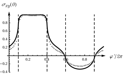
Figure 4: Hall conductance in units of $q^{2}/h$ following a quantum quench from the topological phase with $\varphi=\pi/3$ and $M=1$ (as indicated by the triangular symbol in Fig. 1) to $\varphi=\varphi^{\prime}$ and $M=1$. The gray dots are numerical results for the Haldane model obtained from Eq. (9). The black solid line is the analytical result for the corresponding quenches in the low-energy Dirac approximation, obtained by summing contributions from Eq. (13). The results are in quantitative agreement for small quenches in the vicinity of $\varphi=\pi/3$, and in qualitative agreement for larger quenches. The vertical dashed lines correspond to the boundaries of the topological phases. The Hall conductance remains numerically close to $q^{2}/h$ for quenches within the same topological phase ($\nu=1$), but does not saturate at $-q^{2}/h$ when quenching to the other topological phase ($\nu=-1$).

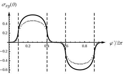
Figure 5: Hall conductance in units of $q^{2}/h$ following a quantum quench from the non-topological phase with $\varphi=\pi$ and $M=1$ (as indicated by the square symbol in Fig. 1) to $\varphi=\varphi^{\prime}$ and $M=1$. The gray dots are numerical results for the Haldane model obtained from Eq. (9). The black solid line is the analytical result for the corresponding quenches in the low-energy Dirac approximation, obtained by summing contributions from Eq. (13). The results are in quantitative agreement for small quenches in the vicinity of $\varphi=\pi$, and in qualitative agreement for larger quenches. The vertical dashed lines correspond to the boundaries of the topological phases.

More generally, we may use Eq. (7) to determine the a.c. Hall response for frequencies smaller than the band gap, $\omega\ll\Delta_{b,b^{\prime}}({\rm k})$; see Fig. 6.

Figure 6: Hall response $\sigma_{xy}(\omega)$ in units of $q^{2}/h$ evaluated using Eq. (7) for frequencies below the direct band gap $\Delta\equiv{\rm min}[\Delta_{b,b^{\prime}}({\bf k})]$, following a quantum quench from the topological phase with $M=1$ and $\varphi=\pi/3$, to the non-topological phase with $M=1$ and $\varphi=\varphi^{\prime}$. The three curves correspond to $\varphi^{\prime}=7\pi/8$ (circles), $\varphi^{\prime}=\pi$ (triangles) and $\varphi^{\prime}=9\pi/8$ (squares), for which $\Delta\sim 0.67$, $2$, and $0.67\times t_{1}/\hbar$, respectively.

For larger frequencies, non-diagonal contributions of the form $c_{b,{\bf k}}c_{b^{\prime},{\bf k}}^{\ast}$ do not disappear under unitary evolution and the current (5) must be employed.

IV.1 Low-Energy Approximation

Analytical results for the Hall response (9) may be obtained within the framework of the low-energy Dirac Hamiltonian for sufficiently small quenches. At low-energies, the Haldane model may be described as the sum of two Dirac Hamiltonians $H=H_{+}+H_{-}$  Haldane (1988) where

$$H_{\alpha}=\begin{pmatrix}m_{\alpha}c^{2}&&-cpe^{i\alpha\theta}\\ -cpe^{-i\alpha\theta}&&-m_{\alpha}c^{2}\end{pmatrix}.$$ (12)

Here, $\alpha=\pm$ labels the two inequivalent Dirac points, $c=3t_{1}a/2\hbar$ is the effective speed of light, $p\exp(i\theta)$ parametrizes the 2D momentum ($p_{x}$,$p_{y}$) and $m_{\alpha}=(M-3\sqrt{3}\alpha t_{2}\sin\varphi)/c^{2}$ is the effective Dirac fermion mass Haldane (1988). In this representation, a quench of the Haldane parameters $M\rightarrow M^{\prime}$ and $\varphi\rightarrow\varphi^{\prime}$ corresponds to quenches of the effective masses $m_{\alpha}\rightarrow m_{\alpha}^{\prime}$. Combining results for the Berry curvature Price and Cooper (2012), with the Dirac band occupation following a quench Caio et al. (2015), one obtains

$$\sigma_{xy}^{\alpha}(0)=\frac{\alpha e^{2}}{2h}\int_{0}^{\infty}dp\frac{cpm_{\alpha}^{\prime}(p^{2}+c^{2}m_{\alpha}m_{\alpha}^{\prime})}{\sqrt{p^{2}+c^{2}m_{\alpha}^{2}}{(p^{2}+c^{2}{m_{\alpha}^{\prime}}^{2})}^{2}},$$ (13)

for the two Dirac points. This is in agreement with Refs Wang and Kehrein (2015); Wang et al. (2016). In deriving this result, the integral over the two-dimensional Brillouin zone has been replaced by an integral over the infinite two-dimensional momentum-space. The solid lines in Figs 4 and  5 correspond to the low-energy approximation $\sigma_{xy}(0)=\sigma_{xy}^{+}(0)+\sigma_{xy}^{-}(0)$. The approximation is in good agreement with the exact numerical results for the lattice model (1). For small quenches, which do not explore the non-linear regime of the dispersion relation, the results agree quantitatively. For larger quenches, the approximation breaks down, but it still captures the qualitative features. For large quenches, with $\lvert m-m^{\prime}\rvert\rightarrow\infty$, the contribution to the Hall conductance from a single Dirac point shows plateaus at $(\pm\pi/8)q^{2}/h$; see Fig. 7. These results are consistent with the notion that preservation of $\nu$ does not imply the preservation of the Hall response $\sigma_{xy}(0)$. In the absence of interactions, the final state is non-thermal, and characterized by the occupations $c_{b,{\bf k}}$ in Eq. (9). In this excited state the Hall response need not be quantized.

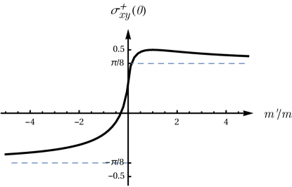
Figure 7: Post-quench Hall conductance in units of $q^{2}/h$ for a single Dirac point ($\alpha=+$), following a quench from $m>0$ to $m^{\prime}$. For the same choice of quench parameters, the other Dirac point ($\alpha=-$) displays the opposite Hall conductance. Note that for quenches in the Haldane model, the changes in mass for each Dirac point may differ, yielding a non-zero Hall response. The dashed lines correspond to the asymptotes $\sigma_{xy}(0)=\pm(\pi/8)q^{2}/h$, which can be determined analytically from Eq. (13).

V Generalized Gibbs Ensemble

A quantitative description of the non-thermal post-quench state can be obtained by considering the system in a cylindrical geometry with open boundary conditions along one direction; see Fig. 8. In our previous work we showed that the resulting edge currents undergo non-trivial dynamics, due to the presence or absence of edge modes in the spectrum Caio et al. (2015).

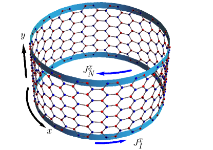
Figure 8: Finite-size cylindrical geometry with periodic (open) boundary conditions along the $x$- ($y$-) direction. When $\varphi\neq 0$ there are generically edge currents, $J_{1}^{x}$ and $J_{N}^{x}$, flowing along the sample boundaries in opposite directions. After a quantum quench, the edge currents evolve as a function of time, and currents flow into the interior of the sample.

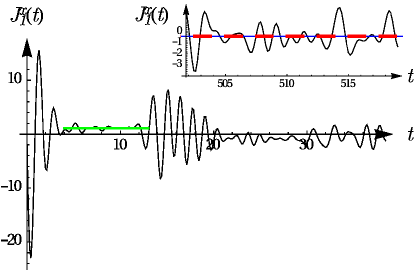
Figure 9: (Main) Total edge current $J_{1}^{x}(t)$ in units of $qt_{1}a/\hbar$ following a quantum quench within the topological phase with $\nu=-1$. The time $t$ is measured in units of $\hbar/t_{1}$. We set $\varphi=\pi/3$ and quench $M$ from $1.4$ to $-1.4$. The solid horizontal (green) line corresponds to the time-averaged total edge current, in the quasi-stationary regime before the onset of finite-size traversals. (Inset) Late-time data after $29$ traversals of the sample. The dashed (red) line corresponds to the prediction of the GGE. This agrees with the time-average of the late-time data, as shown by the solid horizontal line (blue), to within approximately $3\%$.

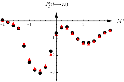
Figure 10: Comparison of the time-averaged total edge current in the Haldane model at late times (circles) and the prediction $\Braket{\hat{\rho}_{{\rm GGE}}\hat{J}^{x}_{1}}$ of the GGE (triangles) for quantum quenches with $\varphi=\pi/3$ held fixed and $M=1.4\rightarrow M^{\prime}$. The time averaging is performed over a single traversal period of the finite-size system, following $29$ traversals of the sample. The currents are measured in units of $qt_{1}a/\hbar$.

In particular, the edge currents decay towards new values that depend on the post-quench Hamiltonian, and not just the initial state; see Fig. 9. This evolution is accompanied by light-cone spreading of currents into the interior of the sample, with the eventual onset of finite-size effects and resurgent oscillations. Here, we show that the long time behavior of the total edge current, after many traversals of the sample, is captured by a Generalized Gibbs Ensemble (GGE) Rigol et al. (2007, 2008); Caux and Konik (2012). The density matrix is given by

$$\hat{\rho}_{{\rm GGE}}=Z^{-1}\exp{\left(-\sum_{\gamma}\lambda_{\gamma}\hat{n}_{\gamma}\right)},$$ (14)

where $\hat{n}_{\gamma}$ are the conserved occupations of a given energy state, $\gamma$ labels the energy level and the momentum index, and $Z={\rm Tr}\exp{\left(-\sum_{\gamma}\lambda_{\gamma}\hat{n}_{\gamma}\right)}$; see Appendix C. Here, the $\lambda_{\gamma}$’s are generalized inverse temperatures. These are determined by the self-consistency condition that the mode occupations immediately after the quench coincide with the averages computed via the GGE, $\Braket{\hat{n}_{\gamma}}={\rm Tr}(\hat{\rho}_{{\rm GGE}}\hat{n}_{\gamma})$. This yields $\lambda_{\gamma}=\ln[(1-\Braket{\hat{n}_{\gamma}})/\Braket{\hat{n}_{\gamma}}]$ Rigol et al. (2007). In Fig. 10 we show the comparison between the time-averaged total edge current along a single edge at late times, and the predictions of the GGE. The results are in excellent agreement.

VI Confinement Potentials

Thus far, we have explored the dynamics of the Haldane model in toroidal and cylindrical geometries, as periodic boundary conditions provide considerable simplifications for theory and simulation. In order to make clear predictions for experiment, it is instructive to consider finite-size samples with open boundaries, especially due to the use of optical traps for cold atoms. We first consider the effects of transverse confinement in the cylindrical geometry depicted in Fig. 8, before discussing the case of rotationally symmetric confinement. For earlier work exploring the effects of trapping potentials on the equilibrium edge physics of topological systems see Refs Stanescu et al. (2010); Buchhold et al. (2012).

We consider the Haldane model in the setup shown in Fig. 8, with an additional harmonic confinement potential applied along the $y$-direction, $V(y)\propto(y-y_{0})^{2}$. Here $y_{0}$ is the center of the trap which we take to be located at the midpoint of the strip. It is convenient to parameterize the potential as

$$V_{n}={\mathcal{C}}\left(\frac{n-N/2}{\zeta-N/2}\right)^{2},$$ (15)

where $n=1,\dots,N$ labels the row of the strip, $\zeta$ controls the effective width of the confined sample, and ${\mathcal{C}}$ is a constant. For suitable choices of ${\mathcal{C}}$ and $\zeta$, for a strip of a given width $N$, the equilibrium particle density is approximately uniform for $\zeta<n<N-\zeta$; see Fig. 11(a). The corresponding current profile in the topological phase shows clearly separated edge currents that are broadened due to the smooth confinement potential; see Fig. 11(b). In contrast to the case of hard wall boundaries Caio et al. (2015), the bulk also contains longitudinal Hall currents if it corresponds to a topological phase with non-zero Chern number. These arise due to the effective transverse electric field generated by the harmonic potential.

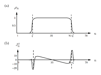
Figure 11: Equilibrium properties of the Haldane model in the cylindrical geometry shown in Fig. 8, with an additional harmonic confinement potential $V_{n}$ given by Eq. 15. We consider the topological phase with $M=0$ and $\varphi=\pi/3$ and set $N=70$, $\mathcal{C}=1.2$ and $\zeta=15$. (a) Particle density $\rho_{n}$ as a function of the row index $n\in 1,...,70$. At half-filling, the potential confines the particles into the region $\zeta<n<N-\zeta$, as indicated by the vertical dashed lines. This imposes an effective system size in which it is possible to observe edge effects. (b) Total longitudinal current $J_{n}^{x}$ along the cylinder showing clearly separated edge currents, broadened due to the smooth potential. Hall currents exist in the interior of the sample due to the effective electric field generated by the trap.

Following a quantum quench, the edge currents spread towards the interior of the sample, as found in the case of hard wall boundaries Caio et al. (2015); see Fig. 12. The currents also spread outside the initial sample area to a lesser extent due to the harmonic confinement. The light-cone propagation is clearly visible in the presence of the trap, but the apparent speed of light differs slightly from the uniform case. This is attributed to the broadening of the edge current profiles and the presence of the equilibrium bulk Hall currents, induced by the harmonic potential.

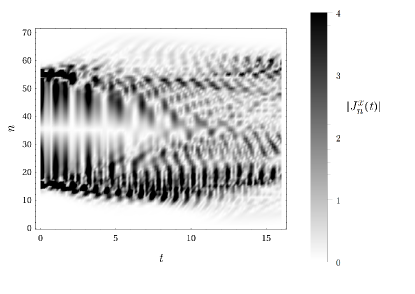
Figure 12: Dynamics of the currents $|J_{n}^{x}(t)|$ following a quantum quench from the topological phase with $M=0$ and $\varphi=\pi/3$ to the non-topological phase $M=3$ and $\varphi=\pi/3$. We set $N=70$, $\mathcal{C}=1.2$ and $\zeta=15$. The spreading of the currents into the interior (and to a lesser extent the exterior) of the effective sample is visible even in the presence of the harmonic potential. However, the propagation speed departs from the effective speed of light, due to the broadening of the edge currents and the contribution of bulk Hall currents.

The case of fully open boundary conditions presents a significant increase in the numerical computations required, but is not expected to lead to different results. In the presence of a rotationally symmetric harmonic trap, as shown in Fig. 13(a), broadened edge currents will flow on the effective sample boundaries; see Fig. 13(b). Likewise, equilibrium bulk Hall currents will also circulate (in the opposite sense to the edge currents) due to the effective radial electric field. Following a quantum quench, the edge currents will flow towards the interior of the sample, exhibiting light-cone propagation; this will be smoothed out by the edge current broadening and the bulk Hall currents, which are present even in equilibrium.

An estimate of the timescales for the light-cone propagation can be inferred from the experimental parameters used in Ref. Jotzu et al. (2014). Using the typical hopping parameter $t_{1}\sim 10^{2}\,h$Hz, the effective speed of light is $c\sim 10^{3}\,a/\rm{s}$, measured in intersite spacings per second. i.e. lattice site propagation occurs on millisecond timescales. The timescale for observing the onset of the current plateau in Fig. 9, and the light-cone propagation in Fig. 12, is thus of the order of several milliseconds; the unit of time in Figs 9 and 12 is $\hbar/t_{1}\sim 10^{-3}\,\rm{s}$. This is comparable with the timescales explored in experiment Jotzu et al. (2014).

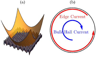
Figure 13: (a) Illustration of the potential landscape of a hexagonal optical lattice in the presence of a rotationally symmetric harmonic trap. (b) Circulating equilibrium currents in the resulting disk geometry. Following a quantum quench between the topological and the non-topological phases the edge currents are expected to propagate into the interior (and the exterior) of the sample at the effective speed of light. This will be smoothed out due to the broadening of the edge currents and the presence of the bulk Hall currents.

VII Conclusions

In this paper we have explored the transport properties of Chern insulators following a quantum quench in an isolated system undergoing unitary evolution. The Hall conductance is no longer described by the ground state relation $\sigma_{xy}(0)=\nu q^{2}/h$, in spite of the preservation of $\nu$ in infinite-size systems; the Chern index is a property of the state, whilst the Hall response depends both on the state and the final Hamiltonian. In the presence of open boundary conditions, the total edge currents are described by a GGE at late times. It would be interesting to explore the quench dynamics of Chern insulators in experiment, probing their Hall response and edge current dynamics.

Appendix A Low-Energy Approximation

In Figs 4 and 5 we compare the post-quench Hall response in the Haldane model (1) with the low-energy Dirac approximation (13). For completeness we provide a derivation of the latter; see also Refs Wang and Kehrein (2015); Wang et al. (2016). For a single Dirac point, the occupation probability amplitudes of the lower and upper bands following an effective mass quench $m\rightarrow m^{\prime}$, are given by Caio et al. (2015)

$$\begin{split}a(m,m^{\prime},p)&=f_{-}(p,m)f_{-}(p,m^{\prime})+f_{+}(p,m)f_{+}(p,m^{\prime}),\\ b(m,m^{\prime},p)&=f_{+}(p,m)f_{-}(p,m^{\prime})-f_{-}(p,m)f_{+}(p,m^{\prime}),\end{split}$$ (16)

respectively, where $f_{\pm}(p,m)\equiv\sqrt{\frac{1}{2}\left(1\pm\frac{mc}{\sqrt{p^{2}+m^{2}c^{2}}}\right)}$. Here we have parameterized the two-dimensional momentum space with $(p,\theta)$, as in the main text. For a single Dirac point $\alpha$, the Berry curvature of the upper band is given by $\alpha\Omega_{\rm D}(p,m)$, where $\Omega_{\rm D}(p,m)=cpm/(p^{2}+m^{2}c^{2})^{3/2}$; the Berry curvature of the lower band has the opposite sign Price and Cooper (2012). Substituting these results into Eq. (9) it follows that after a quench $m_{\alpha}\rightarrow m_{\alpha}^{\prime}$,

$$\sigma_{xy}^{\alpha}(0)=\frac{\alpha q^{2}}{2h}\int_{0}^{\infty}dp\,\Omega_{\rm D}(p,m_{\alpha}^{\prime})\,\times\\ \left(\lvert b(m_{\alpha},m_{\alpha}^{\prime},p)\rvert^{2}-\lvert a(m_{\alpha},m_{\alpha}^{\prime},p)\rvert^{2}\right).$$ (17)

Eq. (13) follows straightforwardly Wang and Kehrein (2015); Wang et al. (2016).

Appendix B Edge Currents

In order to study the dynamics of the edge currents, we consider the Haldane model (1) in a finite-size cylindrical geometry, with periodic (open) boundary conditions along the $x$- ($y$-) direction; see Fig. 8. We define the local current flowing through a site $l$ of the lattice as Caio et al. (2015)

$$\hat{\mathbf{J}}_{l}:=-\frac{iq}{2}\sum_{j}\bm{\delta}_{jl}(t_{lj}\hat{c}_{l}^{{\dagger}}\hat{c}_{j}-{\rm H}.{\rm c}.),$$ (18)

where $t_{lj}$ is the hopping parameter, $\bm{\delta}_{jl}$ is the vector joining site $j$ to $l$, and the sum is performed over nearest and next-nearest neighbors. Each lattice index corresponds to a triplet of indices $\{m=1,...,M;n=1,...,N;s=A,B\}$, labeling the $x$- and $y$- positions of the unit cell, and the sublattice Caio et al. (2015). The total longitudinal current flowing along the lower edge of the cylinder in the $x$-direction is given by $J_{1}^{x}=\langle\hat{J}_{1}^{x}\rangle=\sum_{ms}\langle\hat{J}^{x}_{m1s}\rangle$, as shown in Figs 8 and 9.

Appendix C Generalized Gibbs Ensemble

In the finite-size cylindrical geometry depicted in Fig. 8, the Hamiltonian can be diagonalized as $\hat{H}=\sum_{\Upsilon,k_{x}}\epsilon_{\Upsilon}(k_{x}){\hat{f}}^{{\dagger}}_{\Upsilon}(k_{x}){\hat{f}}^{\mathstrut}_{\Upsilon}(k_{x})$, where we have exploited the periodicity in the $x$-direction, and $\Upsilon=1,\dots,2N$ labels the energy levels at each $k_{x}$-point. In the non-interacting model (1) the number operators $\hat{n}_{\Upsilon}(k_{x})={\hat{f}}^{{\dagger}}_{\Upsilon}(k_{x}){\hat{f}}^{\mathstrut}_{\Upsilon}(k_{x})$ are conserved. Denoting the pair of indices $\{\Upsilon,k_{x}\}$ by $\gamma$, the late-time values of the time-averaged edge currents are described by the GGE given in Eq. (14).

References

- Klitzing et al. (1980) K. Klitzing, G. Dorda, and M. Pepper, Phys. Rev. Lett. 45, 494 (1980).
- Laughlin (1981) R. Laughlin, Phys. Rev. B 23, 5632 (1981).
- Thouless et al. (1982) D. Thouless, M. Kohmoto, M. Nightingale, and M. den Nijs, Phys. Rev. Lett. 49, 405 (1982).
- Niu et al. (1985) Q. Niu, D. J. Thouless, and Y.-S. Wu, Phys. Rev. B 31, 3372 (1985).
- Murthy and Shankar (2003) G. Murthy and R. Shankar, Rev. Mod. Phys. 75, 1101 (2003).
- Novoselov et al. (2005) K. S. Novoselov, A. K. Geim, S. V. Morozov, D. Jiang, M. I. Katsnelson, I. V. Grigorieva, S. V. Dubonos, and A. A. Firsov, Nature 438, 197 (2005).
- Zhang et al. (2005) Y. Zhang, Y.-W. Tan, H. L. Stormer, and P. Kim, Nature 438, 201 (2005).
- Kane and Mele (2004) C. L. Kane and E. J. Mele, Phys. Rev. Lett. 95, 226801 (2004).
- Bernevig et al. (2006) B. A. Bernevig, T. L. Hughes, and S.-C. Zhang, Science 314, 1757 (2006).
- König et al. (2007) M. König, S. Wiedmann, C. Brüne, A. Roth, H. Buhmann, L. W. Molenkamp, X.-L. Qi, and S.-C. Zhang, Science 318, 766 (2007).
- Khanikaev et al. (2013) A. B. Khanikaev, S. H. Mousavi, W.-K. Tse, M. Kargarian, A. H. MacDonald, and G. Shvets, Nat. Mater. 12, 233 (2013).
- Fu and Kane (2008) L. Fu and C. Kane, Phys. Rev. Lett. 100, 096407 (2008).
- Kitagawa et al. (2010) T. Kitagawa, E. Berg, M. Rudner, and E. Demler, Phys. Rev. B 82, 235114 (2010).
- Lindner et al. (2011) N. H. Lindner, G. Refael, and V. Galitski, Nat. Phys. 7, 490 (2011).
- Rechtsman et al. (2013) M. C. Rechtsman, J. M. Zeuner, Y. Plotnik, Y. Lumer, D. Podolsky, F. Dreisow, S. Nolte, M. Segev, and A. Szameit, Nature 496, 196 (2013).
- Foster et al. (2013) M. S. Foster, M. Dzero, V. Gurarie, and E. A. Yuzbashyan, Phys. Rev. B 88, 104511 (2013).
- Foster et al. (2014) M. S. Foster, V. Gurarie, M. Dzero, and E. A. Yuzbashyan, Phys. Rev. Lett. 113, 076403 (2014).
- D’Alessio and Rigol (2015) L. D’Alessio and M. Rigol, Nat. Commun. 6, 8336 (2015).
- Caio et al. (2015) M. D. Caio, N. R. Cooper, and M. J. Bhaseen, Phys. Rev. Lett. 115, 236403 (2015).
- Wang and Kehrein (2015) P. Wang and S. Kehrein, (2015), arXiv:1504.05689 .
- Wang et al. (2016) P. Wang, M. Schmitt, and S. Kehrein, Phys. Rev. B 93, 085134 (2016).
- Haldane (1988) F. D. M. Haldane, Phys. Rev. Lett. 61, 2015 (1988).
- Jotzu et al. (2014) G. Jotzu, M. Messer, R. Desbuquois, M. Lebrat, T. Uehlinger, D. Greif, and T. Esslinger, Nature 515, 237 (2014).
- Rigol et al. (2007) M. Rigol, V. Dunjko, V. Yurovsky, and M. Olshanii, Phys. Rev. Lett. 98, 050405 (2007).
- Rigol et al. (2008) M. Rigol, V. Dunjko, and M. Olshanii, Nature 452, 854 (2008).
- Caux and Konik (2012) J.-S. Caux and R. M. Konik, Phys. Rev. Lett. 109, 175301 (2012).
- Chern (1946) S.-S. Chern, Ann. Math. Second Ser. 47, 85 (1946).
- Berry (1984) M. V. Berry, Proc. R. Soc. A 392, 45 (1984).
- Note (1) We are grateful to Prof. B. I. Halperin for this argument.
- Nakagawa et al. (2016) Y. O. Nakagawa, G. Misguich, and M. Oshikawa, (2016), arXiv:1601.06167 .
- Dehghani et al. (2015) H. Dehghani, T. Oka, and A. Mitra, Phys. Rev. B 91, 155422 (2015).
- Karplus and Luttinger (1954) R. Karplus and J. M. Luttinger, Phys. Rev. 95, 1154 (1954).
- Kohn and Luttinger (1957) W. Kohn and J. M. Luttinger, Phys. Rev. 108, 590 (1957).
- Xiao et al. (2010) D. Xiao, M.-C. Chang, and Q. Niu, Rev. Mod. Phys. 82, 1959 (2010).
- Chang and Niu (1995) M. Chang and Q. Niu, Phys. Rev. Lett. 75, 1348 (1995).
- Price and Cooper (2012) H. M. Price and N. R. Cooper, Phys. Rev. A 85, 033620 (2012).
- Aidelsburger et al. (2014) M. Aidelsburger, M. Lohse, C. Schweizer, M. Atala, J. Barreiro, S. Nascimbène, N. Cooper, I. Bloch, and N. Goldman, Nat. Phys. 11, 162 (2014).
- Hu et al. (2016) Y. Hu, P. Zoller, and J. C. Budich, (2016), arXiv:1603.00513 .
- Wilson et al. (2016) J. H. Wilson, J. C. W. Song, and G. Refael, (2016), arXiv:1603.01621 .
- Stanescu et al. (2010) T. D. Stanescu, V. Galitski, and S. Das Sarma, Phys. Rev. A 82, 013608 (2010).
- Buchhold et al. (2012) M. Buchhold, D. Cocks, and W. Hofstetter, Phys. Rev. A 85, 063614 (2012).