The Riemann Mapping Theorem from Riemann’s Viewpoint

Abstract.

This article presents a rigorous proof of the Riemann Mapping Theorem via Riemann’s method, uncompromised by any appeals to topological intuition.

The Riemann Mapping Theorem is one of the most remarkable results of nineteenth century mathematics. Even today, more than a hundred fifty years later, the fact that every proper simply connected open subset of the complex plane is biholomorphically equivalent to every other seems deep and profound. This is not a result that has become in any sense obvious with the passage of time and the general expansion of mathematics. And at the time, the theorem must have been truly startling. Even Gauss, never easily impressed, viewed the result favorably, though he had reservations about the summary nature of Riemann’s writings. At the time, Riemann’s method appeared hard to carry out in detail. And indeed there have been those since who believed it could not be carried out in detail at all.

Thus, when a different proof arose later on using Montel’s idea of normal families, this proof established itself as standard [2]. Indeed, it is rare to find any other proof than the normal families one in contemporary texts on complex analysis. Only if the student of complex analysis goes on to study uniformization of open Riemann surfaces is Riemann’s original idea likely to be encountered. At best, the original proof idea is relegated to exercises or brief summaries in texts on basic complex analysis (cf., e.g., Exercise 73, p. 251 in [4], or Section 5.2, p. 249-251 in [1]).

And yet, in the historical view, Riemann’s proposed method of proof was as interesting and perhaps even more important than the result itself. It would have been almost impossible for anyone listening to Riemann’s presentation in 1851 to have imagined that what they were hearing was the first instance of a mathematical method that would become a massive part of geometric mathematics in the decades to come and that continues to be a vitally active subject today. But so it was, for Riemann’s proof method for his mapping theorem marked the introduction of the use of elliptic equations and the solution of elliptic variational problems to treat geometric questions. The analytic theory of Riemann surfaces via harmonic forms and Hodge’s generalization to algebraic varieties in higher dimensions; the circle of results known by the name the Bochner technique; the theory of minimal submanifolds and its applications to topology of manifolds; the use of elliptic methods in 4-manifold theory; and, most recently, the proof of the Poincaré Conjecture and the geometrization conjecture that extends it—all these and much more could not have been anticipated in any detail on that historic day at the time Riemann presented his mapping theorem. But in retrospect, when Riemann suggested constructing the biholomorphic map to the unit disc that his result called for by solving an elliptic variational problem, the whole development began. The fact that Riemann could not in fact actually prove what he called Dirichlet’s Principle is almost beside the point. He had found the way into the thicket. Chopping the path onward could be and would be done by others.

Thus, it seemed to the authors unfortunate that finding a precise and complete discussion of how actually to carry out Riemann’s argument is not easy. Osgood’s proof [7] of the Riemann Mapping Theorem—usually regarded as the first reasonably complete proof, correct except for certain topological details being brushed over—does indeed use Riemann’s general idea. But it is made more difficult than need be today because he was not in possession of the Perron method of solving the Dirichlet problem. Thus he had to work with piecewise linear approximations from the interior and take limits of the piecewise linear (even piecewise real analytic) case of the Dirichlet problem that had been solved by Schwarz already at that time [13].

Our goal in this article is to present a clear proof of the Riemann Mapping Theorem via Riemann’s method, uncompromised by any appeals to topological intuition. Such intuitions are notoriously unreliable and, even if correct, can be surprisingly hard to substantiate. Moreover, one of the most intriguing features of the Riemann Mapping Theorem is that it provides a proof of the strictly topological fact that any simply connected open subset of the plane is homeomorphic to any other. Since one wishes to deduce this topological conclusion, it is particularly desirable not to appeal to any unproven topological facts in the proof of the Riemann Mapping Theorem itself. (That simple connectivity of a domain in the plane implies homeomorphism to the plane [or the disc] can be shown directly, cf. Theorem 6.4, p. 149 in [6]—but it is a delicate and intricate matter).

The basic method is Riemann’s, but in the intervening years the Perron solution of the Dirichlet problem for any bounded domain with barriers at each boundary point has simplified the basic construction. That there are barriers at each point of the boundary of a simply connected bounded open set in $\mathbb{C}$ does hold. This was in effect pointed out by Osgood, though the barrier terminology was not in use at that time. Putting this together with some arguments about winding numbers and counting preimages will complete the proof.

Acknowledgments. The authors are indebted to D. Marshall for helpful comments about a preliminary version of this paper, in regard to weak and strong barriers in particular.

1. The Theorem’s exact statement and the first steps in the proof

The Theorem as we shall prove it is about simply connected open subsets of the plane $\mathbb{C}$. People usually interpret “simply connected” in this context to mean topologically simply connected, i.e., that the open set is connected and also that every continuous closed curve in the open set can be continuously deformed inside the open set to a constant curve. As it happens, we shall end up proving a slightly different result which, on the face of it, is stronger. Namely, we shall assume about the open set only that it is connected and has the property that every holomorphic function on it has a (holomorphic) anti-derivative. That is, if $f$ is a holomorphic function on the open set then there is a holomorphic function $F$ on the set with $F^{\prime}=f$. We shall say then that $U$ is holomorphically simply connected.

It is easy to show that topological simple connectivity as defined implies the holomorphic anti-derivative property just described. The theorem itself in the following form will show among other things the converse, namely, that the holomorphic simple connectivity implies topological simple connectivity.

Theorem 1.1 (Riemann).

Suppose that $U$ is a connected open subset of $\mathbb{C}$ with $U\neq\mathbb{C}$. If $U$ is holomorphically simply connected, then $U$ is biholomorphic to the unit disc, i.e., there is a one-to-one holomorphic function from $U$ onto the unit disc $D=\{z\in\mathbb{C}\colon|z|<1\}$.

In the proof of this result, it will be useful to be able to assume that $U$ is bounded. For this, we recall the familiar fact that such a $U$ as in the theorem is always biholomorphic to a bounded open set. The proof of this in summary form goes like this. Since $U\neq\mathbb{C}$ , we can replace $U$ by a translate to suppose that $0\notin U$. The function $1/z$ is then holomorphic on $U$ and hence has an antiderivative $L(z)$, say. Changing $L$ by an additive constant will arrange that $\exp(L(z))=z$ (this is the usual process for finding complex logarithms). Then $\exp(L(z)/2)$ is one-to-one on $U$. Choose an open disc in the image of $\exp(L(z)/2)$. The negative of this disc is disjoint from the image of $\exp(L(z)/2)$. So the image of $\exp(L(z)/2)$, which is biholomorphic to $U$, is itself biholomorphic to a bounded open subset of $\mathbb{C}$, via a linear fractional transformation.

Note that it is not clear by definition that the holomorphic simple connectivity is preserved by a biholomorphic mapping since the meaning of taking the derivative is different when the coordinates change; but by the complex chain rule this is a matter of a holomorphic factor which can be assimilated into the original function. Checking the details of this is left to the reader as an exercise.

So now we can assume without loss of generality that the open set $U$ is bounded. And by translation we can now assume $0\in U$. We shall look for a biholomorphic mapping from $U$ to the unit disc $D$ which takes 0 to 0. Of course if there is a biholomorphic map from $U$ to the unit disc at all, there is one that takes 0 to 0 since a linear fractional transformation taking the unit disc $D$ to itself will take any given point to the origin, and in particular the image of 0 to begin with can be moved to the origin.

Now if $H\colon U\to D$ is biholomorphic and has $H(0)=0$, then $H(z)/z$ has a removable singularity at 0 . Hence $H$ can be written as $zh(z)$ where $h$ is holomorphic on $U$ and $h(0)\neq 0$. That $h(0)\neq 0$ follows because $H$ is supposed to be one-to-one and hence must have derivative vanishing nowhere. Of course $h(z)$ is also nonzero for every other $z\in U$ because 0 is the only point of $U$ with $H(z)=0$,

Now there is an antiderivative $L$ of $h^{\prime}/h$ on $U$. The product$h(z)\exp(-L(z))$ is constant since it has derivative identically equal to 0 and $U$ is connected. Changing $L$ by an additive constant, we can assume $h(z)\exp(-L(z))=1$ for all $z\in U$. (This familiar argument will occur several times here).

The essential point of Riemann’s method was to consider the harmonic function $\text{Re}\,L(z)$. This is of course equal to $\ln|h(z)|$. Since the “boundary values” of $|H(z)|$ have to be 1, it must be that the boundary value of $|h|$ at a boundary point $z_{0}$ of $U$ has to be $1/|z_{0}|$. In particular, the harmonic function $\ln|h|$ has to have boundary value at $z_{0}$ equal to $-\ln|z_{0}|$.

At this point, Riemann appealed to what he referred to as the Dirichlet Principle. The Euler-Lagrange equation for the variational problem of minimizing the so-called Dirichlet (energy) integral for a real valued function $f(x,y)$, namely minimizing this integral

$$\int_{U}\bigg{[}\Big{(}\frac{\partial f}{\partial x}\Big{)}^{2}+\Big{(}\frac{\partial f}{\partial y}\Big{)}^{2}\bigg{]}~{}dxdy$$

under the condition that $f=g$ on the boundary $\partial U$ of $U$, is easily computed to satisfy $\Delta f=0$ (§18 of [11, 12]).

So Riemann proposed that the harmonic function with the boundary values $-\ln|z_{0}|$ at each boundary point $z_{0}$ could be found by minimization of the Dirichlet integral. And Riemann was well aware of how to construct $h$ and hence $H$ from knowing $\ln|h(z)|$. Riemann actually expressed this all in terms of $\ln|H|$ and the idea of Green’s function, a function with boundary value 0 and a specified singularity at (in our case) the point 0, namely the function had to be of the form $\ln|z|+u(z)$ with $u$ harmonic near the point 0. This is equivalent for open sets in $\mathbb{C}$ to our discussion, though the Green’s function notion is useful when one tries to extend the Riemann Mapping Theorem to the uniformization problem where there is no a priori global $z$-coordinate.

The main difficulty is that there is no particular reason to suppose that there is in fact any minimum for the Dirichlet integral in this situation. There is also a less serious difficulty of explaining why the resulting function is one-to-one and onto—intuitively this is just a matter of winding numbers if one can approximate $U$ from the inside by domains with smooth or piecewise-smooth closed curve boundaries. One supposes that Riemann may have taken this part for obvious, though it is actually quite subtle if one does not appeal to any pre-existing topological intuitions. We shall give a precise argument later on. Riemann apparently considers only domains the boundary of which is smooth in some sense. Osgood made the major forward step treating simply connected open sets in general, thus proving what we call today the Riemann Mapping Theorem. The Osgood proof is acknowledged directly by Carathéodory [2] where the ideas involved in the usual proof of today, via normal families, are presented. See the footnote (**) of page 108 of [2]. But for some reason, Osgood’s proof fell from favor or even recognition for the history of the Theorem in [10]; there is a reference to Osgood’s paper but no comment on it, no acknowledgment that this is in fact the reasonably complete first proof of the general result.

2. The Application of the Perron Method

Even simply connected bounded open sets in $\mathbb{C}$ can have complicated boundaries. The boundary of the Koch snowflake for example has Hausdorff dimension greater than 1 [5]. And Osgood [7] already gave an example with boundary having positive (2-dimensional) measure. Thus it is appropriate to introduce carefully what is to be meant by finding functions with specified boundary values. For this purpose, let $U$ be a bounded open set in $\mathbb{C}$ and $\partial U$ be its boundary, that is the complement of $U$ within the closure $\operatorname{cl}(U)$ of $U$ in $\mathbb{C}$, or equivalently the intersection of $\operatorname{cl}(U)$ with $\mathbb{C}-U$. Suppose that $b\colon\partial U\to\mathbb{R}$ is a continuous function, Then we say that a harmonic function $h\colon U\to\mathbb{R}$ is a solution of the Dirichlet problem on $U$ with boundary values $b$ if the function “$h\cup b$” is continuous on $\operatorname{cl}(U)$. Here $h\cup b$ is the function which equals $h$ on $U$ and equals $b$ on $\operatorname{cl}(U)-U$.

The Maximum Principle shows immediately that if a given Dirichlet problem has a solution, the solution is unique. But it is a fact that given $U$ and a function $b$ on $\partial U$, there may be no solution of the associated Dirichlet problem. This is familiar but disconcerting in the present context since solving a Dirichlet problem is the basic step in Riemann’s approach to the Riemann Mapping Theorem, as already indicated. The easiest example of a Dirichlet problem with no solution is $\{z\in\mathbb{C}\colon 0<|z|<1\}$ with $b(0)=0$ and $b(z)=1$ if $|z|=1$. The reason for the failure is simple. Uniqueness shows that any solution $h(z)$ would have to depend on $|z|$ alone: the problem is rotationally symmetric so the solution would have to be. But the only such harmonic functions have the form $A\ln|z|+B$ where $A$ and $B$ are constants. This follows easily by looking at the Laplacian in polar coordinates. But clearly no such function solves the Dirichlet problem mentioned.

The open set $\{z\in\mathbb{C}\colon 0<|z|<1\}$ is not simply connected. And it turns out that on a bounded simply connected open set $U$, the Dirichlet problem is solvable for every boundary function $b$. This is the crucial piece of information needed in Riemann’s proof. This fact fits into a very general context. It turns out that the Dirichlet problem with arbitrary boundary function $b$ will be solvable provided that no connected component of the complement of $U$ consists of a single point. Since a simply connected open set (in the topological sense) has a connected but unbounded complement, the complement’s one and only component cannot consist of a single point! However, these points—the condition on the complement that guarantees the solution of the Dirichlet problem and the fact that the complement of a simply connected open set is connected—are hard to establish. Fortunately, a much simpler argument can be used to show that the Dirichlet problem is always solvable on a bounded simply connected open set. This involves only the Perron method, which has become a standard part of basic complex analysis courses. We can stay on familiar ground here.

In the more than seventy years from Riemann’s formulation of his Mapping Theorem to Perron’s paper [8] on the solution of the Dirichlet problem under the most general possible circumstances, results had been obtained on the solution of the Dirichlet problem for open sets with various conditions of boundary regularity. In particular, Schwarz [13] had shown that the problem was solvable if the boundary was piecewise analytic. Every bounded open set $U$ can be approximated by open subsets $V$ with piecewise linear boundaries. For instance, as we shall discuss in detail momentarily, such $V$ can be taken to be a union of squares contained in $U$. In effect, one lays a finely divided piece of graph paper (a fine grid of squares) over $U$ and takes $V$ to be the union of all the squares whose closure lies in $U$. This method was used by Osgood [7] to construct a Green function for $U$ relative to some fixed but arbitrary point of $U$ by taking a limit of Green’s functions of the sets $V$ of the sort just described, as one chose finer and finer grids on the plane. In this process, simple connectivity was used (as indeed it had to be) in order to guarantee the convergence, and the form in which it was used was closely related to the barrier idea that occurs in Perron’s method.

In Perron’s method, one begins with a bounded open set $U$ and a function $b$ on $\partial U$ as before. Then one offers as a candidate for the solution of the associated Dirichlet problem the function $P$ on $U$ defined by $P(z)=\sup S(z)$, where the sup is taken over all (continuous) subharmonic functions $S\colon U\to R$ satisfying $\displaystyle\limsup_{U\ni p_{j}\to q}S(p_{j})\leq b(q)$ for each $q\in\partial U$.

This function $P$ is always harmonic. But of course it need not have the function $b$ as boundary values. I.e., it need not happen that $P\cup b$ is continuous on $\operatorname{cl}(U)$. This has to fail in some instances, since the Dirichlet problem is not always solvable.

Perron undertook to find a general condition under which $P$ did have $b$ as boundary values. This condition involves the existence of what have come to be called barrier functions.

Definition 2.1.

Suppose that $U$ is a bounded open set in $\mathbb{C}$ and $\zeta_{0}$ is a boundary point of $U$. A strong barrier, or sometimes just barrier, at $\zeta_{0}$ is a continuous function $u$ defined on $\{z\in\mathbb{C}\colon|z-\zeta_{0}|<\epsilon\}\cap U$ for some $\epsilon>0$ such that

• $u$ is subharmonic.

• $u<0$.

• $\displaystyle\lim_{z\to\zeta_{0}}u(z)=0$ with limit taken over all $z$ in the domain of $u$.

• $\displaystyle\limsup_{z\to\zeta}u(z)<0$ for every $\zeta\in\partial U\cap\{z\in\mathbb{C}\colon 0<|z-\zeta_{0}|<\epsilon\}$.

A weak barrier is a function $u$ satisfying the same conditions except that the property (iv) is omitted.

Perron’s solution of the Dirichlet problem is usually presented in complex analysis textbooks under the assumption that the bounded domain $U$ has the property that there is a strong barrier at each boundary point. However, G. Bouligand showed soon after Perron’s original work that in fact it was enough to have a weak barrier at each boundary point.

Theorem 2.2 (Perron-Bouligand).

If $U$ is a bounded connected open set in $\mathbb{C}$ with the property that for each boundary point $\zeta_{0}$ of $U$, there is a weak barrier defined on an open disc around $\zeta_{0}$, then, for any continous function $b$ on the boundary $\partial U$ of $U$, the Perron upper envelope function $P$ associated to $b$ solves the Dirichlet problem on $U$ with boundary values $b$, i.e., $P$ is harmonic on $U$ and $P\cup b$ is continous on $U\cup\partial U$.

The details of this result can be found in [15] and other standard texts on potential theory, e.g. [9, 14].

Now we turn to the fact that weak barriers necessarily exist at boundary points of bounded open sets which are holomorphically simply connected. This is perhaps at first sight surprising since this condition of holomorphic simple connectivity seems to have nothing much to do with the existence of barriers. The argument goes as follows. (This is essentially due to Osgood in [7]):

Let $q$ be a point of $\partial U$. Then the function $D_{q}(z)=z-q$, has no zeros in $U$ and hence there is a function $L(z)$ such that $\exp(L(z))=D_{q}(z)=z-q$ by an argument already discussed. This requires only the holomorphic simple connectivitiy of $U$.

Then the function $L$ is one-to-one on $U$ since $L(z_{1})=L(z_{2})$ implies $\exp L(z_{1})=\exp(L(z_{2}))$ so that $z_{1}-q=z_{2}-q$ and so $z_{1}=z_{2}$. Hence $L$ is a biholomorphic map of $U$ onto $L(U)$. The open set $L(U)$ is unbounded because $\text{Re}\,L(z)=\ln|z-q|$ goes to $-\infty$ as $z$ approaches $q$. (Note here that, by choice, $q$ is in $\partial U$ so there are sequences of points in $U$ that approach $q$). On the other hand, there is a positive real number $A$ such that $\text{Re}\,L(z)<A$ for all $z\in U$. This is just because $U$ is bounded so $|z-q|$ is bounded on $U$ and $\text{Re}\,L(z)=\ln|z-q|$. It follows that $U$ can be mapped biholomorphically onto a bounded open set $V$ which is contained in a disc bounded by a circle $C$ through 0 with 0 being in the boundary of the image of $U$ and with 0 corresponding to the boundary point $q$. The precise meaning of this last is that for every sequence $z_{j}$ in $U$ converging to $q$, the image sequence converges to 0.

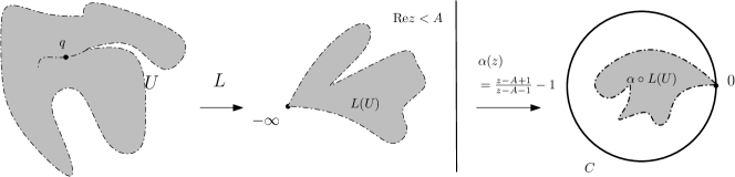
Figure 1. A weak barrier at $q\in\partial U$

This biholomorphic mapping is obtained by composing $L$ with a linear fractional transformation, say $\alpha$, that maps the line $\text{Re}\,z=A$ to a circle in $\mathbb{C}$ in such a way that the image $L(U)$ lies in the bounded component of the complement of the circle. ($L(U)$ lies in the complement in the Riemann sphere of $\{z\colon\text{Re}\,z=A\}\cup\{\infty\}$). The image of $L(q)$ via the linear fractional mapping $\alpha$ will then be the point 0, and the point 0 lies on the the unit circle $C$.

The weak barrier for $U$ at the boundary point $q$ is now obtained by choosing an harmonic function which is 0 at 0 and negative on the circle $C$ and its interior. This could be chosen as a real linear function, for example. Then one pulls this function back to $U$ by the composition of $L$ followed by the linear fractional transformation.

This barrier construction combined with the Perron-Bouligand result quoted guarantees that there is a harmonic function on any bounded holomorphically simply connected open set with $h$ having the boundary value $-\ln|z_{0}|$ for each $z_{0}\in\partial U$, with $U$ as in the first section. We turn now to how to construct from this the biholomorphic map from $U$ to the unit disc $D$ and to the proof that the map constructed actually is biholomorphic.

3. The construction of $H$ and the proof that $H$ is biholomorphic

We continue the notations and conventions of the first section now. Let $g(z)$ be the harmonic function on $U$ which has the boundary values $-\ln|z_{0}|$ at each boundary point $z_{0}$ of $U$. From this, we want to construct the function $h(z)$, which was presumed in the first section to exist as a matter of motivation. Now we want to show that there is actually an $h(z)$ like that, with $H(z)=zh(z)$ being a biholomorphic map to the unit disc.

For this purpose, let $\hat{g}(z)$ be a harmonic conjugate of $g$, i.e., a function such that $g+i\hat{g}$ is holomorphic. The holomorphic simple connectivity of $U$ implies the existence of $\hat{g}$ as follows: The function $\frac{\partial g}{\partial x}-i\frac{\partial g}{\partial y}$ is holomorphic on $U$ by the Cauchy-Riemann equations. If $G$ is a holomorphic anti-derivative of this function, and $G=u+iv,$ then $\frac{\partial u}{\partial x}=\text{Re}\,\frac{\partial G}{\partial x}=\text{Re}\,\frac{\partial G}{\partial z}=\frac{\partial g}{\partial x}$ and $\frac{\partial u}{\partial y}=-\frac{\partial v}{\partial x}=-\text{Im}\,\frac{\partial G}{\partial z}=-\big{(}-\frac{\partial g}{\partial y}\big{)}=\frac{\partial g}{\partial y}$. Thus $u$ and $g$ have the same partial derivatives. Hence $g+iv$ is holomorphic so we can take $\hat{g}$ to be $v$.

Now set $h(z)=\exp(g(z)+i\hat{g}(z))$ and $H(z)=zh(z)$. Then the function $H$ attains the value 0 exactly once, at $z=0$, and with multiplicity 1 there. Also, $|H(z)|$ has boundary value 1 on $U$ in the sense that $|H|\cup(\text{the constant function }1\text{ on }\partial U)$ is continuous. This function $H$ is our candidate for being a biholomorphic map of $U$ onto the unit disc $D=\{z\colon|z|<1\}$. It remains to see that this $H$ really is such a biholomorphic map.

If $U$ were the interior of a smooth simple closed curve then one could envision a simple proof by considering the winding number around a given $w$ in the unit disc of a slight push-in of the boundary of $U$. If the boundary were pushed in a small enough amount, then the image of the pushed-in boundary would be close to the edge of the unit disc. In particular, the line from 0 to $w$ would fail to intersect this image. Thus the number of times that this image curve wound around $w$ would be the same as the number of times that the image curve wound around 0, namely once, since the value 0 is attained exactly once inside the pushed-in curve in $U$ (we assume the push-in is small enough that 0 is inside the pushed-in curve).

This is a valid intuition. One rather suspects that Riemann envisioned the situation in this way. Unfortunately, this intuitive picture, while it can be made precise easily in the smooth boundary case, does not really apply to the general case. Moreover, the idea that a simply connected region has a single boundary curve is not an easy one to check in detail. It is precisely such topological leaps of faith that we want to avoid. So we have to maneuver a bit to make a formal version of this intuition that makes no appeals to unverified and perhaps unverifiable topological intuitions.

We shall provide a somewhat lengthy but not fundamentally difficult argument. We shall replace the push-in boundary curve by a boundary curve made up of the sides of squares. But we shall not need anything about the analogue of the push-in being the boundary of anything with specified properties. It might for example have several components or have self-intersections. We now proceed with the detailed construction.

First, for each positive integer $N$, consider all the closed squares in the plane of the form

$$S_{N}^{n_{1},n_{2}}=\Big{\{}x+iy\in\mathbb{C}:~{}\frac{n_{1}}{2^{N}}\leq x\leq\frac{n_{1}+1}{2^{N}},\ \ \frac{n_{2}}{2^{N}}\leq y\leq\frac{n_{2}+1}{2^{N}}\Big{\}}.$$

Here $n_{1}$ and $n_{2}$ are integers but not necessarily positive integers. These squares cover the plane and any two distinct ones intersect at most at a vertex or an edge of each. We set $T_{N}=$ the collection of triples $(N,n_{1},n_{2})$ such that the associated square $S_{N}^{n_{1},n_{2}}$ is completely contained in $U$ and $S_{N}=$ the union of these associated squares.

Note that each square has a natural orientation so that it makes sense for example to integrate a complex valued function continuous in a neighborhood of the union of the edges of the square around the four edges taken together as a closed curve. Now suppose that $f$ is a complex valued function which is continuous in a neighborhood of all the edges of squares labeled by elements in $T_{N}$. Then the sum of the integrals over the edges of each of the squares $S_{N}^{n_{1},n_{2}}$, $(N,n_{1},n_{2})\in T_{N}$, is defined. If an edge is shared by two squares in this collection, it occurs in one square with opposite orientation from the orientation it has from the other square. Thus we arrive at the result that the sum of the integrals of the four-edge boundary curves of the squares associated to $T_{N}$ equals the integral of the function around the boundary edges of $S_{N}$, where a boundary edge is by definition one which occurs in one of the $S_{N}^{n_{1},n_{2}}$ squares with $(N,n_{1},n_{2})\in T_{N}$ but is not shared with any other $T_{N}$ square.

Figure 2. The squares $S_{N}^{n_{1},n_{2}}$ and the set $S_{N}$

If $K$ is any compact subset in $U$ then there is an $N_{K}>0$ so large that, if $N\geq N_{K}$, then $K$ is contained in $S_{N}$. This follows from the fact that the interiors of the $S_{N}$ form an increasing sequence of open sets with union equal to $U$. With these ideas in mind, we formulate as a lemma the basic result we shall use. The lemma refers back to the function $H$ defined in the previous section.

Lemma 3.1.

Suppose that $r$ is a real number with $0<r<1$. Then there is an $N_{r}>0$ such that, if $N\geq N_{r}>0$, then the interior of $S_{N}$ contains $H^{-1}(\{z\colon|z|\leq r\})$. Moreover. for any such fixed $N>N_{r}$, the number of times that $H$ attains a value $w\in S_{N}$ with $|w|<r$ (and hence the number of times it attains the value $w$ in $U$) is exactly the integral $\displaystyle\frac{1}{2\pi i}\int\frac{H^{\prime}(z)}{H(z)-w}dz$ around the boundary edges of $S_{N}$.

Proof.

The first statement follows easily from the fact that $\ln|H|$ has boundary values 0 on $U$. This implies immediately that there is a $\delta$ such that $|H(z)|>r$ at every point $z\in U$ with $\operatorname{dist}(z,\partial U)<\delta$ (this comes from uniform continuity of the function $|H|\cup 1$ on $U\cup\partial U$. If $N_{r}$ is so large that the diameter of the squares of side length $2^{-N}$ is less than $\delta$, then the first conclusion holds since being outside of $S_{N}$ would imply distance to the boundary of $U$ less than $\delta$ so that no point outside $S_{N}$ could have $H$ image with absolute value less than $r$.

The second conclusion is more or less immediate if no point on the sides of the square labeled by $T_{N}$ contains a point in the inverse image of $w$: for each $T_{N}$ labeled square, the integral $\displaystyle\frac{1}{2\pi i}\int\frac{H^{\prime}(z)}{H(z)-w}dz$ around the edges of the square counts the number of preimages (counting multiplicity) of $w$ inside the square. The total number of preimages of $w$ is obtained by adding up the numbers in each of the $T_{N}$ labeled squares and this gives the integral $\displaystyle\frac{1}{2\pi i}\int\frac{H^{\prime}(z)}{H(z)-w}dz$ around the boundary edges.

This argument does not apply if a preimage of $w$ is actually on the edge of a square labeled in $T_{N}$. However, since the set of preimages of $w$ must be finite in number (since they all lie in a compact set), we can deal with this problem as follows: Redo the whole construction with the squares with the center of the square grid at $(\lambda,\lambda)$, where $\lambda$ is a positive number very close to 0 so that the squares are of the form

$$S_{N}^{n_{1},n_{2}}(\lambda)=\Big{\{}x+iy\in\mathbb{C}: ~{}\frac{n_{1}}{2^{N}}+\lambda\leq x\leq\frac{n_{1}+1}{2^{N}}+\lambda,$$

$$\quad\frac{n_{2}}{2^{N}}+\lambda\leq y\leq\frac{n_{2}+1}{2^{N}}+\lambda\Big{\}}.$$

If $\lambda$ is close enough to 0, it will still be true that the union $S_{N}(\lambda)$ of the squares $S_{N}^{n_{1},n_{2}}(\lambda)$, $(N,n_{1},n_{2})\in T_{N}$, is contained in $U$. It will also be the case that the interior of the union $S_{N}(\lambda)$ contains $H^{-1}(\{w\colon|w|\leq r\})$, again for all $\lambda>0$ small enough. And for a fixed $w$ with $|w|\leq r$, one can arrange that the edges of these $T_{N}$ labeled squares do not contain any preimage of $w$ so that the previous case applies. However, the integral $\displaystyle\frac{1}{2\pi i}\int\frac{H^{\prime}(z)}{H(z)-w}dz$ around the boundary edges of $S_{N}(\lambda)$ is a continous function of $\lambda$ so that, as $\lambda$ is made to approach 0, one obtains the desired conclusion as a limit. ∎

The point here is that preimages of $w$ might lie on interior edges of the $T_{N}$ labeled squares but they cannot lie on the boundary edges so that the integral over the union of the boundary edges is a continuous function of $w$.

Now we can complete the argument that $H$ attains each value $w$ in the unit disc exactly once. Given $w$ with $|w|<1$, choose an $r$ with $|w|<r<1$. The Lemma shows that the number of $H^{-1}(z)$ of a point $z$ in the set $\{z\colon|z|<r\}$ is integer-valued and moreover, since it is given by the integral $\displaystyle\frac{1}{2\pi i}\int\frac{H^{\prime}(z)}{H(z)-w}dz$ over the boundary edges of $S_{N}$ for all suitably large $N$, it must be continuous as a function of $w$. Hence it is everywhere 1 on $\{w\colon|w|<r\}$ because the point 0 has exactly one preimage counting multiplicity, namely the point 0. Thus $H$ attains the alue $w$ exactly once counting multiplicity. Hence $H$ is one-to-one and onto the unit disc. $\Box$

4. Final remarks

4.1.

The argument in this last section is specific to the situation at hand, but the result is in fact a special case of a general consideration, namely that a proper map of one (connected) Riemann surface to another is a branched covering with all points in the image space having the same number of pre-images counting multiplicity. This can be proved by techniques along the same lines as the ones used here for the concrete instance of the Riemann Mapping Theorem.

4.2.

The technique of using harmonic function theory to find biholomorphic mappings of multiply-connected (i.e., not simply connected) open sets in the plane onto model domains has a long and extensive history. The reader might wish to consult [3] for a discussion of the general theory. The thing that is different about simple connectivity is that there is only one model needed (for proper subsets of $\mathbb{C}$). For higher finite-connectivity, the family of models necessarily has a positive number of parameters. These considerations require topological information that is beyond the scope of a short article.

Acknowledgments. The research of the second named author has been supported in part by the SRC-GAIA, an NRF Grant 2011-0030044 of The Republic of Korea.

References

- [1] L. V. Ahlfors: Complex analysis. An introduction to the theory of analytic functions of one complex variable. Second edition. International Series in Pure and Applied Mathematics. McGraw-Hill Book Co. 1966. xiii+317 pp.
- [2] C. Carathéodory: Untersuchungen über die konformen Abbildungen von festen und veränderlichen Gebieten. Math. Ann. 72 (1912), no. 1, 107–144.
- [3] S. D. Fisher: Function theory on planar domains. A second course in complex analysis. John Wiley & Sons, Inc., New York, 1983. xiii+269 pp.
- [4] R. E. Greene and S. G. Krantz: Function theory of one complex variable. Third edition. Graduate Studies in Mathematics 40. American Mathematical Society, 2006. x+504 pp.
- [5] H. von Koch: Une méthode géométrique élémentaire pour l’étude de certaines questions de la théorie des courbes planes. Acta Math. 30 (1906), no. 1, 145–174.
- [6] M. H. A. Newman: Elements of the topology of plane sets of points. 2nd ed. Cambridge University Press, 1951. vii+214 pp.
- [7] W. Osgood: On the existence of the Green’s function for the most general simply connected plane region. Trans. Amer. Math. Soc. 1 (1900), no. 3, 310–314.
- [8] O. Perron: Eine neue Behandlung der ersten Randwertaufgabe für Δu=0. Math. Z. 18 (1923), no. 1, 42–54.
- [9] T. Ransford: Potential theory in the complex plane. Cambridge Univ. Press, 2003.
- [10] R. Remmert, Classical topics in complex function theory. Translated from the German by Leslie Kay. Grad. Texts in Math., 172. Springer-Verlag, New York, 1998. xx+349 pp.
- [11] B. Riemann: Grundlagen für eine allgemeine Theorie der Funktionen einer veränderlichen complexen Grösse, Inaugraldissertation, Göttingen 1851. Zweiter unveränderter Abdruck, Göttinger 1867.
- [12] : Gesammelte Mathematische Werke (2nd ed.), Teubner, Leibzig, 1892; reprinted with additional commentaries (R. Narasimhan ed.). The dissertation is pp. 3–43 in Teubner ed. and pp. 35–75 in Springer ed.
- [13] H. A. Schwarz; Conforme Abbildung der Oberfläche eines Tetraeders auf die Oberfläche einer Kugel. J. Reine Angew. Math. 70 (1869), 121–136.
- [14] B. Simon: Harmonic analysis. Amer. Math. Soc., 2015.
- [15] M. Tsuji: Potential theory in the modern function theory, Maruzen Co., Tokyo 1959. 590 pp.
- [16] J. Walsh: History of the Riemann mapping theorem. Amer. Math. Monthly 80 (1973), 270–276.