Polarization of massive fermions in a vortical fluid

Abstract

Fermions become polarized in a vortical fluid due to spin-vorticity coupling. Such a polarization can be calculated from the Wigner function in a quantum kinetic approach. Extending previous results for chiral fermions, we derive the Wigner function for massive fermions up to the next-to-leading order in spatial gradient expansion. The polarization density of fermions can be calculated from the axial vector component of the Wigner function and is found to be proportional to the local vorticity $\boldsymbol{\omega}$. The polarizations per particle for fermions and anti-fermions decrease with the chemical potential and increase with energy (mass). Both quantities approach the asymptotic value $\hbar\boldsymbol{\omega}/4$ in the large energy (mass) limit. The polarization per particle for fermions is always smaller than that for anti-fermions, whose ratio of fermions to anti-fermions also decreases with the chemical potential. The polarization per particle on the Cooper-Frye freeze-out hyper-surface can also be formulated and is consistent with the previous result of Becattini et al..

I Introduction

In non-central high-energy heavy-ion collisions, the large orbital angular momentum present in the colliding system can lead to non-vanishing local vorticity in the hot and dense fluid Liang and Wang (2005a, b); Becattini et al. (2008); Betz et al. (2007); Gao et al. (2008); Huang et al. (2011). The vorticity induced by global orbital angular momentum in the fluid can be considered as local rotational motion of particles Becattini et al. (2008); Betz et al. (2007); Jiang et al. (2016); Deng and Huang (2016). It is closely related to the rapidity dependence of the $v_{1}$ flow and shear of the longitudinal flow velocity inside the reaction plane Gao et al. (2008); Csernai et al. (2011); Wang et al. (2013).

As a result of spin-orbital coupling, quarks and anti-quarks can become polarized along the normal direction of the reaction plane Liang and Wang (2005a, b); Gao et al. (2008). Through hadronization of polarized quarks and anti-quarks, hyperons can also be polarized in the same direction in the final state Liang and Wang (2005a, b); Becattini et al. (2013a). Measurements of such global hyperon polarization is feasible through the parity-violating decay of hyperons Abelev et al. (2007); Deng (2014). Such measurements will shed light on properties of the vortical structures of the strongly coupled quark-gluon plasma (sQGP) in high-energy heavy-ion collisions.

Quark and anti-quark polarization in a vortical fluid is also closely related to the Chiral Magnetic and Vortical Effects Kharzeev et al. (2008); Fukushima et al. (2008); Son and Surowka (2009); Kharzeev and Son (2011); Pu et al. (2011); Gao et al. (2012). From the solutions of Wigner functions for chiral or massless fermions in a quantum kinetic approach one can derive the axial current $j_{5}^{\mu}=\rho_{5}u^{\mu}+\xi_{5}\omega^{\mu}+\xi_{5}^{B}B^{\mu}$, where $\rho_{5}$ is the axial charge density, $u^{\mu}$ is the fluid velocity, $\omega^{\mu}\equiv\frac{1}{2}\epsilon^{\mu\sigma\alpha\beta}u_{\sigma}\partial_{\alpha}u_{\beta}$ is the vorticity 4-vector, and $B^{\mu}=\frac{1}{2}\epsilon^{\mu\nu\lambda\sigma}u_{\nu}F_{\lambda\sigma}$ is the 4-vector of the magnetic field with $F_{\lambda\rho}$ being the strength tensor of the electromagnetic field. The coefficients $\xi_{5}$ and $\xi_{5}^{B}$ are all functions of temperatures and chemical potentials $\mu$ and $\mu_{5}$ Gao et al. (2012). In a three-flavor quark matter with u, d and s quarks and their anti-quarks, $\xi_{5}^{B}=0$. In other words, the axial current in a three-flavor quark matter is blind to the magnetic field and solely induced by the vorticity. Such an axial current leads to the Local Polarization Effect Gao et al. (2012) which is also connected to the spin-vorticity coupling for chiral or massless fermions Gao and Wang (2015).

In this paper, we will extend our Wigner function method for massless fermions to massive ones and formulate the polarization of massive fermions induced by vorticity. In Section II, we will give a brief introduction to the Wigner function method and derive the equations for the Wigner function components for massive fermions based on Ref. Elze et al. (1986); Vasak et al. (1987). The Wigner function components can be determined perturbatively by gradient expansion. In Section III, we will derive the Wigner function at the leading order by definition. Using the projection method we can extract each component of the Wigner function at the leading order. We will propose the first order solution for the axial vector component in Section IV by extending the solution for massless fermions. In Section V, we will show that the axial vector component can be regarded as the spin density in phase space. We can obtain the polarization density after completion of momentum integration of the axial vector component in Section VI. We will also formulate the fermion polarization on the freezeout hypersurface by extending the Cooper-Frye formula. We will give a summary of the results in the final section.

We adopt the same sign conventions for fermion charge $Q$ as in Refs. Vasak et al. (1987); Gao et al. (2012); Chen et al. (2013); Gao and Wang (2015), and the same sign convention for the axial vector $A^{\mu}\sim\left\langle\bar{\psi}\gamma^{\mu}\gamma^{5}\psi\right\rangle$ as in Resf. Gao et al. (2012); Chen et al. (2013); Gao and Wang (2015) but different sign convention from Ref. Vasak et al. (1987).

II Wigner function for massive fermions

In this section we will give a brief introduction to the Wigner function and its kinetic equation for massive fermions based on Refs. Elze et al. (1986); Vasak et al. (1987). There are also other earlier works in the literature along this line Zhuang and Heinz (1996); Ochs and Heinz (1998). In a background electromagnetic field, the quantum mechanical analogue of a classical phase-space distribution for fermions is the gauge invariant Wigner function $W_{\alpha\beta}(x,p)$ defined by

$$W_{\alpha\beta}(x,p)=\int\frac{d^{4}y}{(2\pi)^{4}}e^{-ip\cdot y}\left\langle\bar{\psi}_{\beta}(x+\frac{1}{2}y)PU(G,x+\frac{1}{2}y,x-\frac{1}{2}y)\psi_{\alpha}(x-\frac{1}{2}y)\right\rangle,$$ (1)

where $\psi_{\alpha}$ and $\bar{\psi}_{\beta}$ are fermionic quantum fields, $\langle\hat{O}\rangle$ denotes the grand canonical ensemble averaging and normal ordering, $x=(x_{0},\mathbf{x})$ and $p=(p_{0},\mathbf{p})$ are time-space and energy-momentum 4-vectors respectively, and the gauge link $PU(G,x_{1},x_{2})$ is to ensure the gauge invariance of the Wigner function and given by

$$PU(G,x+\frac{1}{2}y,x-\frac{1}{2}y)=P\exp\left[-iQy^{\mu}\int_{0}^{1}dsG_{\mu}(x-\frac{1}{2}y+sy)\right],$$ (2)

where $G^{\mu}$ is the gauge potential of the classical electromagnetic field.

The Wigner function in (1) satisfies the following equation of motion,

$$(\gamma_{\mu}K^{\mu}-m)W(x,p)=0,$$ (3)

where the operator $K^{\mu}$ is given by

$$K^{\mu}=p_{\mathrm{W}}^{\mu}+i\hbar\frac{1}{2}\nabla^{\mu},$$ (4)

with

$$p_{\mathrm{W}}^{\mu} = p^{\mu}-\hbar\frac{1}{2}Qj_{1}(\Delta)F^{\mu\nu}\partial_{p\,\nu},$$

$$\nabla^{\mu} = \partial_{x}^{\mu}-Qj_{0}(\Delta)F^{\mu\nu}\partial_{p\,\nu},$$ (5)

where we have used $\Delta\equiv\frac{1}{2}\hbar\partial_{p}\cdot\partial_{x}$ with the operator $\partial_{x}$ in $\Delta$ acting only on the strength tensor $F^{\mu\nu}$, and $j_{0}(x)=\mathrm{sin}(x)/x$ and $j_{1}(x)=(\mathrm{sin}(x)-x\mathrm{cos}(x))/x^{2}$ are spherical Bessel functions. If $F^{\mu\nu}$ is a constant we have simpler forms of these operators

$$p_{\mathrm{W}}^{\mu} = p^{\mu},$$

$$\nabla^{\mu} = \partial_{x}^{\mu}-QF^{\mu\nu}\partial_{p\,\nu}.$$ (6)

The Wigner function is a $4\times 4$ matrix in Dirac indices and can be decomposed into 16 independent generators of Clifford algebra,

$$W=\frac{1}{4}\left[F+i\gamma^{5}P+\gamma^{\mu}V_{\mu}+\gamma^{5}\gamma^{\mu}A_{\mu}+\frac{1}{2}\sigma^{\mu\nu}S_{\mu\nu}\right],$$ (7)

where the generators of Clifford algebra are

$$\Gamma_{i}=1,\gamma^{5}=i\gamma^{0}\gamma^{1}\gamma^{2}\gamma^{3},\gamma^{\mu},\gamma^{5}\gamma^{\mu},\sigma^{\mu\nu}=\frac{i}{2}[\gamma^{\mu},\gamma^{\nu}],$$ (8)

corresponding to the scalar, pseudoscalar, vector, axial vector and tensor components respectively. The coefficients in the decomposition (7) can be obtained by projection of corresponding Dirac matrices on the Wigner function and taking traces,

$$F = \mathrm{Tr}[W],$$

$$P = -i\mathrm{Tr}[\gamma^{5}W],$$

$$V^{\mu} = \mathrm{Tr}[\gamma^{\mu}W],$$

$$A^{\mu} = \mathrm{Tr}[\gamma^{\mu}\gamma^{5}W],$$

$$S^{\mu\nu} = \mathrm{Tr}[\sigma^{\mu\nu}W].$$ (9)

Substituting Eq. (7) into Eq. (3) with (6) and comparing common terms in the basis of Clifford algebra, we obtain the following system of equations,

$$K^{\mu}V_{\mu}-mF = 0,$$

$$K^{\mu}A_{\mu}+imP = 0,$$

$$K_{\mu}F+iK^{\nu}S_{\nu\mu}-mV_{\mu} = 0,$$

$$iK_{\mu}P+\frac{1}{2}\epsilon_{\mu\beta\nu\sigma}K^{\beta}S^{\nu\sigma}+mA_{\mu} = 0,$$

$$-i(K_{\mu}V_{\nu}-K_{\nu}V_{\mu})-\epsilon_{\mu\nu\alpha\beta}K^{\alpha}A^{\beta}-mS_{\mu\nu} = 0.$$ (10)

The real parts of the above equations are

$$p^{\mu}V_{\mu}-mF = 0,$$

$$\frac{1}{2}\hbar\nabla^{\mu}A_{\mu}+mP = 0,$$

$$p_{\mu}F-\frac{1}{2}\hbar\nabla^{\nu}S_{\nu\mu}-mV_{\mu} = 0,$$

$$-\frac{1}{2}\hbar\nabla_{\mu}P+\frac{1}{2}\epsilon_{\mu\beta\nu\sigma}p^{\beta}S^{\nu\sigma}+mA_{\mu} = 0,$$

$$\frac{1}{2}\hbar(\nabla_{\mu}V_{\nu}-\nabla_{\nu}V_{\mu})-\epsilon_{\mu\nu\alpha\beta}p^{\alpha}A^{\beta}-mS_{\mu\nu} = 0.$$ (11)

The imaginary parts are

$$\hbar\nabla^{\mu}V_{\mu} = 0,$$

$$p^{\mu}A_{\mu} = 0,$$

$$\frac{1}{2}\hbar\nabla_{\mu}F+p^{\nu}S_{\nu\mu} = 0,$$

$$p_{\mu}P+\frac{1}{4}\hbar\epsilon_{\mu\beta\nu\sigma}\nabla^{\beta}S^{\nu\sigma} = 0,$$

$$(p_{\mu}V_{\nu}-p_{\nu}V_{\mu})+\frac{1}{2}\hbar\epsilon_{\mu\nu\alpha\beta}\nabla^{\alpha}A^{\beta} = 0.$$ (12)

From the 3rd and the 5th line of the imaginary part equations (12) we obtain,

$$p\cdot\nabla F = 0,$$ (13)

and

$$\hbar(\nabla^{\lambda}A^{\rho}-\nabla^{\rho}A^{\lambda})-2\epsilon^{\mu\nu\lambda\rho}p_{\mu}V_{\nu} = 0,$$ (14)

respectively, where we have multiplied $\epsilon^{\mu\nu\lambda\rho}$ to the equation and used $\epsilon^{\mu\nu\lambda\rho}\epsilon_{\mu\nu\alpha\beta}=-2(\delta_{\alpha}^{\lambda}\delta_{\beta}^{\rho}-\delta_{\beta}^{\lambda}\delta_{\alpha}^{\rho})$. Taking contraction of the above equation with $p^{\lambda}$, we obtain

$$p\cdot\nabla A^{\rho} = p_{\lambda}\nabla^{\rho}A^{\lambda}=QF^{\rho\xi}A_{\xi},$$ (15)

where we have used $p^{\mu}A_{\mu}=0$ from the 2nd line of Eqs. (12).

From the 1st and 3rd lines of real part equations (11), we obtain

$$(p^{2}-m^{2})F = \frac{1}{2}\hbar p^{\mu}\nabla^{\nu}S_{\nu\mu}\approx\frac{1}{2}\hbar QF^{\mu\nu}S_{\mu\nu},$$ (16)

where we have neglected the second order term $\hbar\nabla^{\nu}(p^{\mu}S_{\nu\mu})\sim\hbar^{2}$. Inserting the 5th line into the 4th line in Eqs. (11) and neglecting the second order term $\hbar\nabla_{\mu}P\sim\hbar^{2}$, we obtain

$$(p^{2}-m^{2})A_{\mu} = \frac{1}{2}\hbar\epsilon_{\mu\beta\nu\sigma}p^{\beta}\nabla^{\nu}V^{\sigma}$$ (17)

$$= -\frac{1}{2}\hbar Q\epsilon_{\mu\beta\nu\sigma}F^{\beta\nu}V^{\sigma}=-\hbar Q\tilde{F}_{\mu\sigma}V^{\sigma}.$$

where we have neglected the second order term $\hbar\epsilon_{\mu\beta\nu\sigma}\nabla^{\nu}(p^{\beta}V^{\sigma})\sim\hbar^{2}$ following the last line of Eqs. (12). Here we have used $\tilde{F}^{\rho\lambda}=\frac{1}{2}\epsilon^{\rho\lambda\mu\nu}F_{\mu\nu}$.

From the 2nd, 3rd and 5th lines of Eqs. (11), the pseudoscalar, vector and tensor components are

$$P = -\frac{1}{2m}\hbar\nabla^{\mu}A_{\mu},$$

$$V_{\mu} = \frac{1}{m}p_{\mu}F-\frac{1}{2m}\hbar\nabla^{\nu}S_{\nu\mu},$$

$$S^{\nu\sigma} = \frac{1}{2m}\hbar(\nabla^{\nu}V^{\sigma}-\nabla^{\sigma}V^{\nu})-\frac{1}{m}\epsilon^{\nu\sigma\alpha\beta}p_{\alpha}A_{\beta}.$$ (18)

Substituting the above into Eqs. (16,17), we obtain a closed system of on-shell equations for $F$ and $A^{\mu}$ up to $O(\hbar)$. We now collect all equations for $F$ and $A^{\mu}$,

$$p^{\mu}A_{\mu} = 0,$$

$$p\cdot\nabla A^{\rho} = QF^{\rho\xi}A_{\xi},$$

$$p\cdot\nabla F = 0,$$

$$(p^{2}-m^{2})F = -\frac{1}{2m}\hbar QF_{\mu\nu}\epsilon^{\mu\nu\alpha\beta}p_{\alpha}A_{\beta},$$

$$(p^{2}-m^{2})A_{\mu} = -\frac{1}{m}\hbar Q\tilde{F}_{\mu\sigma}p^{\sigma}F,$$ (19)

which make a closed system of equations for $F$ and $A^{\mu}$ and can be solved perturbatively in powers of $\hbar$. The last two equations relate the solutions of the lower order to the higher order. Having $F$ and $A^{\mu}$, we can determine $P$, $V^{\mu}$ and $S^{\mu\nu}$ through Eq. (18).

III Wigner function components at leading order

At leading order of electromagnetic interaction, the gauge link in the Wigner function in Eq. (1) can be set to 1, then we have following simple form

$$W_{\alpha\beta}(x,p)=\int\frac{d^{4}y}{(2\pi)^{4}}e^{-ip\cdot y}\left\langle\bar{\psi}_{\beta}(x+\frac{y}{2})\psi_{\alpha}(x-\frac{y}{2})\right\rangle.$$ (20)

We can expand fermionic fields in momentum space using creation and destruction operators as

$$\psi(x) = \frac{1}{\sqrt{\Omega}}\sum_{\mathbf{k},s}\frac{1}{\sqrt{2E_{k}}}[a(\mathbf{k},s)u(\mathbf{k},s)e^{-ik\cdot x}+b^{\dagger}(\mathbf{k},s)v(\mathbf{k},s)e^{ik\cdot x}],$$

$$\bar{\psi}(x) = \frac{1}{\sqrt{\Omega}}\sum_{\mathbf{k},s}\frac{1}{\sqrt{2E_{k}}}[a^{\dagger}(\mathbf{k},s)\bar{u}(\mathbf{k},s)e^{ik\cdot x}+b(\mathbf{k},s)\bar{v}(\mathbf{k},s)e^{-ik\cdot x}],$$ (21)

where $\Omega$ is the volume and $s=\pm$ denote the spin state parallel or anti-parallel to the spin quantization direction $\mathbf{n}$ in the rest frame of the particle. Insert the above into Eq. (20), we obtain

$$W_{\alpha\beta}(x,p) = \frac{1}{(2\pi)^{3}}\delta(p^{2}-m^{2})\bigg{\{}\theta(p^{0})\sum_{s}f_{\mathrm{FD}}(E_{p}-\mu_{s})u_{\alpha}(\mathbf{p},s)\bar{u}_{\beta}(\mathbf{p},s)$$ (22)

$$-\theta(-p^{0})\sum_{s}f_{\mathrm{FD}}(E_{p}+\mu_{s})v_{\alpha}(-\mathbf{p},s)\bar{v}_{\beta}(-\mathbf{p},s)\bigg{\}},$$

where we have used $\left\langle a^{\dagger}(\mathbf{p},s)a(\mathbf{p},s)\right\rangle=f_{\mathrm{FD}}(E_{p}-\mu_{s})$ and $\left\langle b^{\dagger}(-\mathbf{p},s)b(-\mathbf{p},s)\right\rangle=f_{\mathrm{FD}}(E_{p}+\mu_{s})$ with the Fermi-Dirac distribution defined by $f_{\mathrm{FD}}=1/(e^{\beta x}+1)$ ($\beta\equiv 1/T$, $T$ is temperature) and $\mu_{s}$ is the chemical potential for the fermions with spin state $s$.

From Eq. (22) we can extract the scalar, vector and axial vector components by applying Eq. (9). We extract the scalar component as

$$F_{(0)} = \mathrm{Tr}[W]=m\delta(p^{2}-m^{2})V$$ (23)

where we have used $\bar{u}(\mathbf{p},s)u(\mathbf{p},s)=2m$ and $\bar{v}(-\mathbf{p},s)v(-\mathbf{p},s)=-2m$, and

$$V\equiv\frac{2}{(2\pi)^{3}}\sum_{s}\left[\theta(p^{0})f_{\mathrm{FD}}(p_{0}-\mu_{s})+\theta(-p^{0})f_{\mathrm{FD}}(-p_{0}+\mu_{s})\right].$$ (24)

For the vector component, we have

$$V_{(0)}^{\mu} = \mathrm{Tr}[\gamma^{\mu}W]=p^{\mu}\delta(p^{2}-m^{2})V,$$ (25)

where we have used $\bar{u}(\mathbf{p},s)\gamma^{\mu}u(\mathbf{p},s)=2(E_{p},\mathbf{p})$ and $\bar{v}(-\mathbf{p},s)\gamma^{\mu}v(-\mathbf{p},s)=2(E_{p},-\mathbf{p})$. For the axial vector component, we obtain

$$A_{(0)}^{\mu} = \mathrm{Tr}[\gamma^{\mu}\gamma^{5}W]$$ (26)

$$= m\left[\theta(p_{0})n^{\mu}(\mathbf{p},\mathbf{n})-\theta(-p_{0})n^{\mu}(-\mathbf{p},-\mathbf{n})\right]\delta(p^{2}-m^{2})A,$$

where we have defined

$$A\equiv\frac{2}{(2\pi)^{3}}\sum_{s}s\left[\theta(p^{0})f_{\mathrm{FD}}(p_{0}-\mu_{s})+\theta(-p^{0})f_{\mathrm{FD}}(-p_{0}+\mu_{s})\right],$$ (27)

and used $\bar{u}(\mathbf{p},s)\gamma^{\mu}\gamma^{5}u(\mathbf{p},s)=2msn^{\mu}(\mathbf{p},\mathbf{n})$ and $\bar{v}(-\mathbf{p},s)\gamma^{\mu}\gamma^{5}v(-\mathbf{p},s)=2msn^{\mu}(-\mathbf{p},-\mathbf{n})$ with $n^{\mu}(\mathbf{p},\mathbf{n})$ given by

$$n^{\mu}(\mathbf{p},\mathbf{n}) = \Lambda_{\;\nu}^{\mu}(\mathbf{v})n^{\nu}(\mathbf{0},\mathbf{n})=\left(\frac{\mathbf{n}\cdot\mathbf{p}}{m},\mathbf{n}+\frac{(\mathbf{n}\cdot\mathbf{p})\mathbf{p}}{m(m+E_{p})}\right).$$ (28)

Here $\Lambda_{\;\nu}^{\mu}(\mathbf{v})$ is the Lorentz transformation for $\mathbf{v}=\mathbf{p}/E_{p}$ and $n^{\nu}(\mathbf{0},\mathbf{n})=(0,\mathbf{n})$ is the 4-vector of the spin quantization direction in the rest frame of the fermion. One can check that $n^{\mu}(\mathbf{p},\mathbf{n})$ satisfies $n^{2}=-1$ and $n\cdot p=0$, so it behaves like a spin 4-vector up to a factor of 1/2. For Pauli spinors $\chi_{s}$ and $\chi_{s^{\prime}}$ in $u(\mathbf{p},s)$ and $v(-\mathbf{p},s^{\prime})$ respectively, we have $\chi_{s}^{\dagger}\boldsymbol{\sigma}\chi_{s}=s\mathbf{n}$ and $\chi_{s^{\prime}}^{\dagger}\boldsymbol{\sigma}\chi_{s^{\prime}}=-s^{\prime}\mathbf{n}$. We can take the massless limit by setting $\mathbf{n}=\hat{\mathbf{p}}$, then we have $mn^{\mu}(\mathbf{p},\mathbf{n})\rightarrow(|\mathbf{p}|,\mathbf{p})$ and $mn^{\mu}(-\mathbf{p},-\mathbf{n})\rightarrow(|\mathbf{p}|,-\mathbf{p})$. This way we can recover the previous result of the axial vector component for massless fermions Gao et al. (2012); Chen et al. (2013),

$$A_{(0)}^{\mu} \rightarrow \delta(p^{2})\frac{2}{(2\pi)^{3}}p^{\mu}\sum_{s}s\bigg{\{}\theta(p^{0})f_{\mathrm{FD}}(p_{0}-\mu_{s})+\theta(-p^{0})f_{\mathrm{FD}}(-p_{0}+\mu_{s})\bigg{\}},$$ (29)

where $s=\pm$ now denote the right-handed and left-handed fermions.

IV Axial vector component at next-to-leading order

We start with the solution to the Wigner function for chiral or massless fermions Gao et al. (2012); Chen et al. (2013); Gao and Wang (2015). It is well known that in this case the vector and axial vector components decouple from the rest of other components. Their solutions can be recombined into the chiral components of right-hand and left-hand,

$$\mathscr{J}_{(0)s}^{\rho}(x,p) = p^{\rho}f_{s}\delta(p^{2}),$$

$$\mathscr{J}_{(1)s}^{\rho}(x,p) = -\frac{s}{2}\hbar\tilde{\Omega}^{\rho\sigma}p_{\sigma}\frac{df_{s}}{d(\beta p_{0})}\delta(p^{2})-sQ\hbar\tilde{F}^{\rho\lambda}p_{\lambda}f_{s}\frac{\delta(p^{2})}{p^{2}},$$ (30)

where $s=\pm$ denote right-hand/left-hand helicity, $p_{0}\equiv u\cdot p$, $\tilde{\Omega}^{\rho\sigma}=\frac{1}{2}\epsilon^{\rho\sigma\mu\nu}\partial_{\mu}(\beta u_{\nu})$, $\tilde{F}^{\rho\lambda}=\frac{1}{2}\epsilon^{\rho\lambda\mu\nu}F_{\mu\nu}$, and $f_{s}$ are distribution functions of chiral fermions defined by

$$f_{s}(x,p) = \frac{2}{(2\pi)^{3}}\left[\theta(p_{0})f_{\rm FD}(p_{0}-\mu_{s})+\theta(-p_{0})f_{\rm FD}(-p_{0}+\mu_{s})\right].$$ (31)

and

$$\frac{df_{s}}{d(\beta p_{0})} = \frac{2}{(2\pi)^{3}}\left[\theta(p_{0})\frac{d}{d(\beta p_{0})}f_{\rm FD}(p_{0}-\mu_{s})-\theta(-p_{0})\frac{d}{d(-\beta p_{0})}f_{\rm FD}(-p_{0}+\mu_{s})\right].$$ (32)

Note that in the definition of the dual vorticity tensor $\tilde{\Omega}^{\rho\beta}$ in Eq. (30) we have included the factor $\beta=1/T$ inside $\partial_{\mu}$, which is different from the convention (without such a factor) in Refs. Gao et al. (2012); Chen et al. (2013); Gao and Wang (2015). The chiral components in Eq. (30) are related to the vector and axial vector components by

$$V^{\rho}(x,p) = \mathscr{J}_{+}^{\rho}(x,p)+\mathscr{J}_{-}^{\rho}(x,p),$$

$$A^{\rho}(x,p) = \mathscr{J}_{+}^{\rho}(x,p)-\mathscr{J}_{-}^{\rho}(x,p).$$ (33)

Now we try to extend Eq. (30) to massive fermions. We recall that the vector and axial vector components at the leading or zeroth order are given by Eqs. (25) and (26),

$$V_{(0)}^{\mu} = p^{\mu}\delta(p^{2}-m^{2})V,$$

$$A_{(0)}^{\mu} = m\left[\theta(p_{0})n_{\sigma}(\bar{p},n_{0})-\theta(-p_{0})n_{\sigma}(-\bar{p},-n_{0})\right]\delta(p^{2}-m^{2})A,$$ (34)

where $V=f_{+}+f_{-}$ and $A=f_{+}-f_{-}$ are given by Eqs. (24) and (27). Note that we have written relevant quantities in covariant forms with fluid velocity: $p_{0}\rightarrow u\cdot p$, $(0,\mathbf{p})\rightarrow\bar{p}^{\alpha}=p^{\alpha}-(u\cdot p)u^{\alpha}$, $E_{p}=\sqrt{m^{2}-\bar{p}^{2}}=|u\cdot p|$. In particular, we have re-written $n^{\mu}(\mathbf{p},\mathbf{n})$ and $n^{\mu}(-\mathbf{p},-\mathbf{n})$ from Eq. (26) as

$$n^{\mu}(\mathbf{p},\mathbf{n})\rightarrow n^{\mu}(\bar{p},n_{0}) = -\frac{n_{0}\cdot\bar{p}}{m}u^{\mu}+n_{0}^{\mu}-\frac{n_{0\xi}\bar{p}^{\xi}\bar{p}^{\mu}}{m(m+E_{p})},$$

$$n^{\mu}(-\mathbf{p},-\mathbf{n})\rightarrow n^{\mu}(-\bar{p},-n_{0}) = -\frac{n_{0}\cdot\bar{p}}{m}u^{\mu}-n_{0}^{\mu}+\frac{n_{0\xi}\bar{p}^{\xi}\bar{p}^{\mu}}{m(m+E_{p})},$$ (35)

where $n_{0}^{\alpha}=(0,\mathbf{n})$ is the four-vector in the co-moving frame of the fluid cell and satisfies $n_{0}\cdot u=0$. We now propose the following form for the axial component at the first order for massive fermions based on the solution in Eq. (30),

$$A_{(1)}^{\alpha}(x,p) = -\frac{1}{2}\hbar\tilde{\Omega}^{\alpha\sigma}p_{\sigma}\frac{dV}{d(\beta p_{0})}\delta(p^{2}-m^{2})-Q\hbar\tilde{F}^{\alpha\lambda}p_{\lambda}V\frac{\delta(p^{2}-m^{2})}{p^{2}-m^{2}},$$ (36)

where the first term is induced by the vorticity. We can check that the above $A_{(1)}^{\alpha}(x,p)$ satisfies the first and last equation of (19). The kinetic equation, the second equation of Eq. (19), can be imposed for $A_{(1)}^{\alpha}(x,p)$. We will show in the next section that the axial vector can give the spin 4-vector, so we can calculate the polarization density from the vorticity term of $A_{(1)}^{\alpha}(x,p)$ in Eq. (36).

V Energy-momentum and spin tensor/vector density from the Wigner function

The symmetrized Lagrange density for a free Dirac particle is

$$L=\bar{\psi}(\frac{1}{2}i\gamma^{\mu}\overleftrightarrow{\partial}_{\mu}-m)\psi,$$ (37)

where $\overleftrightarrow{\partial}=\overrightarrow{\partial}-\overleftarrow{\partial}$. The energy-momentum tensor can be obtained,

$$T^{\mu\nu} = \frac{\partial L}{\partial(\partial_{\mu}\psi)}\partial^{\nu}\psi+\partial^{\nu}\psi^{\dagger}\frac{\partial L}{\partial(\partial_{\mu}\psi^{\dagger})}-g^{\mu\nu}L$$ (38)

$$= \frac{1}{2}i\bar{\psi}\gamma^{\mu}\overleftrightarrow{\partial}^{\nu}\psi-g^{\mu\nu}\bar{\psi}(\frac{1}{2}i\gamma^{\mu}\overleftrightarrow{\partial}_{\mu}-m)\psi.$$

When taking ensemble average of $T^{\mu\nu}$, we will use the Dirac equation and assume all fields are on-shell. So we have

$$\left\langle T^{\mu\nu}(x)\right\rangle = \frac{1}{2}i\left\langle\bar{\psi}(x)\gamma^{\mu}\overleftrightarrow{\partial}_{x}^{\nu}\psi(x)\right\rangle-g^{\mu\nu}\left\langle\bar{\psi}(\frac{1}{2}i\gamma^{\alpha}\overleftrightarrow{\partial}_{\alpha}-m)\psi\right\rangle$$ (39)

$$= \int d^{4}pp^{\nu}\mathrm{Tr}(\gamma^{\mu}W)-g^{\mu\nu}\int d^{4}p\left[p_{\mu}\mathrm{Tr}(\gamma^{\mu}W)-m\mathrm{Tr}(W)\right]$$

$$= \int d^{4}pp^{\nu}V^{\mu},$$

where we have used $p^{\mu}V_{\mu}=mF$, the first line of Eqs. (11) and

$$W_{\alpha\beta}(x,p) = \int\frac{d^{4}y}{(2\pi)^{4}}e^{-ip\cdot y}\left\langle\bar{\psi}_{\beta}(x+\frac{y}{2})\psi_{\alpha}(x-\frac{y}{2})\right\rangle$$

$$\lim_{y\rightarrow 0}\partial_{y}^{\mu}\left\langle\bar{\psi}_{\beta}(x+\frac{y}{2})\psi_{\alpha}(x-\frac{y}{2})\right\rangle = \frac{1}{2}\left\langle[\partial_{x}^{\mu}\bar{\psi}_{\beta}(x)]\psi_{\alpha}(x)-\bar{\psi}_{\beta}(x)\partial_{x}^{\mu}\psi_{\alpha}(x)\right\rangle$$ (40)

$$= i\int d^{4}pp^{\mu}W_{\alpha\beta}(x,p).$$

The spin tensor density is defined by

$$M^{\alpha\beta}(x) = \psi^{\dagger}(x)\frac{1}{2}\sigma^{\alpha\beta}\psi(x)=\frac{1}{2}\mathrm{Tr}\left[\gamma_{0}\sigma^{\alpha\beta}\psi(x)\bar{\psi}(x)\right].$$ (41)

Taking the ensemble average of the spin tensor, we can also express it in terms of the Wigner function,

$$\left\langle M^{\alpha\beta}(x)\right\rangle = \frac{1}{2}\lim_{y\rightarrow 0}\mathrm{Tr}\left[\gamma_{0}\sigma^{\alpha\beta}\psi(x-\frac{y}{2})\bar{\psi}(x+\frac{y}{2})\right]$$ (42)

$$= \frac{1}{2}\int d^{4}p\mathrm{Tr}\left[\gamma_{0}\sigma^{\alpha\beta}W(x,p)\right].$$

Then we can define the spin tensor component in the Wigner function as

$$M^{\alpha\beta}(x,p) \equiv \frac{1}{2}\mathrm{Tr}\left[\gamma_{0}\sigma^{\alpha\beta}W(x,p)\right]$$ (43)

$$= \frac{1}{2}\left[-\epsilon^{0\alpha\beta\rho}A_{\rho}+ig^{\alpha 0}\mathrm{Tr}(\gamma^{\beta}W)-ig^{\beta 0}\mathrm{Tr}(\gamma^{\alpha}W)\right],$$

where we have used $\gamma^{\mu}\sigma^{\nu\alpha}=i(g^{\mu\nu}\gamma^{\alpha}-g^{\mu\alpha}\gamma^{\nu})+\epsilon^{\mu\nu\alpha\lambda}\gamma^{5}\gamma_{\lambda}$. If we take $\alpha\beta=ij$ (spatial indices), we have a simple relation

$$M^{ij}(x,p) = -\frac{1}{2}\epsilon^{ijk}A_{k}(x,p)=\frac{1}{2}\epsilon^{ijk}A^{k}(x,p),$$ (44)

where $\epsilon_{ijk}$ is 3-dimensional anti-symmetric tensor. The above property can also be seen by the spatial components of $A^{\mu}(x)$

$$A^{i}(x)=\bar{\psi}(x)\gamma^{i}\gamma^{5}\psi(x)=\psi^{\dagger}(x)\gamma^{0}\gamma^{i}\gamma^{5}\psi(x)=\psi^{\dagger}(x)\Sigma_{i}\psi(x),$$ (45)

where $\Sigma_{i}=\mathrm{diag}(\sigma_{i},\sigma_{i})$ with $\sigma_{i}$ being the Pauli matrices. Thus we recognize that $A^{i}(x,p)/2$ corresponds to the spin vector component of the Wigner function from which we can calculate the polarization density.

VI Polarization from axial vector component

We can now calculate the polarization of massive fermions from the axial vector component obtained in Section V. At the leading order, we can obtain the polarization density by integrating $A_{(0)}^{\alpha}$ in Eq. (26) or Eq. (34) over the 4-momentum,

$$\Pi^{\alpha}_{(0)}(x) = \frac{1}{2}\int d^{4}p\>A_{(0)}^{\alpha}(x,p)$$ (46)

$$= \frac{1}{2}m\int\frac{d^{3}p}{(2\pi)^{3}}\frac{1}{E_{p}}\sum_{s}s\left[n^{\alpha}(\bar{p},n_{0})\frac{1}{e^{\beta(E_{p}-\mu_{s})}+1}-n^{\alpha}(-\bar{p},-n_{0})\frac{1}{e^{\beta(E_{p}+\mu_{s})}+1}\right]$$

$$= -\frac{1}{2}u^{\alpha}\int\frac{d^{3}p}{(2\pi)^{3}}\frac{n_{0}\cdot\bar{p}}{E_{p}}\sum_{s}s\left[\frac{1}{e^{\beta(E_{p}-\mu_{s})}+1}-\frac{1}{e^{\beta(E_{p}+\mu_{s})}+1}\right]$$

$$+\int\frac{d^{3}p}{(2\pi)^{3}}\frac{m}{2E_{p}}\left[n_{0}^{\alpha}-\frac{(n_{0}\cdot\bar{p})\bar{p}^{\alpha}}{m(m+E_{p})}\right]\sum_{s}s\left[\frac{1}{e^{\beta(E_{p}-\mu_{s})}+1}+\frac{1}{e^{\beta(E_{p}+\mu_{s})}+1}\right].$$

If $\mu_{s}=\mu$ does not depend on $s$, we see immediately that $\Pi^{\alpha}=0$. In this case the non-vanishing polarization can only come from the first-order contribution from the vorticity term of $A_{(1)}^{\alpha}(x,p)$ in Eq. (36),

$$\Pi^{\alpha}(x) = \Pi^{\alpha}_{(1)}(x)=-\frac{1}{4}\int d^{4}p\hbar\tilde{\Omega}^{\alpha\sigma}p_{\sigma}\frac{dV}{d(\beta p_{0})}\delta(p^{2}-m^{2})$$ (47)

$$= \frac{1}{2}\int\frac{d^{3}p}{(2\pi)^{3}}\hbar\tilde{\Omega}^{\alpha\sigma}\frac{1}{E_{p}}\left\{\left.p_{\sigma}\right|_{p_{0}=E_{p}}\frac{e^{\beta(E_{p}-\mu)}}{[e^{\beta(E_{p}-\mu)}+1]^{2}}-\left.p_{\sigma}\right|_{p_{0}=-E_{p}}\frac{e^{\beta(E_{p}+\mu)}}{[e^{\beta(E_{p}+\mu)}+1]^{2}}\right\}$$

$$= \frac{1}{2}\hbar\omega^{\alpha}\int\frac{d^{3}p}{(2\pi)^{3}}\left\{\frac{e^{\beta(E_{p}-\mu)}}{[e^{\beta(E_{p}-\mu)}+1]^{2}}+\frac{e^{\beta(E_{p}+\mu)}}{[e^{\beta(E_{p}+\mu)}+1]^{2}}\right\},$$

where we have removed the spin dependence in the chemical potential, $\mu_{s}=\mu$, and we have used the fact that the spatial part of $p_{\sigma}$ gives vanishing momentum integral. We see that the polarization density is proportional to the vorticity vector $\omega^{\alpha}=\tilde{\Omega}^{\alpha\sigma}u_{\sigma}$ and is the sum over contributions from fermions and anti-fermions.

We can also obtain the polarization density from the second (electromagnetic field) term of $A_{(1)}^{\alpha}(x,p)$ in Eq. (36),

$$\Pi_{B}^{\alpha}(x) = \frac{1}{2}\hbar Q\int d^{4}p\tilde{F}^{\alpha\lambda}p_{\lambda}V\frac{d}{dp_{0}^{2}}\delta(p^{2}-m^{2})$$ (48)

$$= -\frac{1}{4}\hbar Q\int d^{4}p\tilde{F}^{\alpha\lambda}u_{\lambda}\frac{dV}{dp_{0}}\delta(p^{2}-m^{2})$$

$$= \frac{1}{2}\hbar Q\beta B^{\alpha}\int\frac{d^{3}p}{(2\pi)^{3}}\frac{1}{E_{p}}\left\{\frac{e^{\beta(E_{p}-\mu)}}{[e^{\beta(E_{p}-\mu)}+1]^{2}}-\frac{e^{\beta(E_{p}+\mu)}}{[e^{\beta(E_{p}+\mu)}+1]^{2}}\right\},$$

where we have used $\delta^{\prime}(x)=-\delta(x)/x$ and that the spatial part of $p_{\sigma}$ gives vanishing momentum intergal. Also we have dropped the complete derivative term which is vanishing at the boundary in momentum space.

We see from Eqs. (47,48) that there is a correspondence between $\Pi^{\alpha}(x)$ from the vorticity and $\Pi_{B}^{\alpha}(x)$ from the magnetic field: $E_{p}\omega^{\alpha}\leftrightarrow Q\beta B^{\alpha}$. Note that there is a factor $\beta$ in the definition of $\omega^{\alpha}$, $\omega^{\alpha}\equiv(1/2)\epsilon^{\alpha\rho\mu\nu}u_{\rho}\partial_{\mu}(\beta u_{\nu})$. At zero temperature, the anti-fermion parts in Eqs. (47,48) are vanishing, the momentum integrals can be carried out analytically from the Fermi sphere distribution. The correspondence at zero temperature now becomes $\mu\omega^{\alpha}\leftrightarrow Q\beta B^{\alpha}$, where the $\beta$ factor cancels the one in the definition of $\omega^{\alpha}$ so the correspondence does not have temperature dependence. From such a correspondence, we see that $\Pi_{B}^{\alpha}(x)$ always comes with the charge $Q$ while $\Pi^{\alpha}(x)$ does not, therefore the contributions from fermions and anti-fermions in $\Pi^{\alpha}(x)$ have the same sign while they have opposite signs in $\Pi_{B}^{\alpha}(x)$ since fermions and anti-fermions carry opposite charges.

In this paper we consider only the polarization induced by the vorticity since it lasts longer and is stronger than the magnetic effect in later stage of hydrodynamical evolution for massive hadrons.

To estimate the magnitude of $\Pi^{\mu}(x)$ for fermions from Eq. (47), we can carry out the momentum integral in the co-moving frame. After completing the integral over the momentum direction, we obtain the spin polarization density

$$\boldsymbol{\Pi}(x) = \hbar\boldsymbol{\omega}\frac{1}{4\pi^{2}}\int_{0}^{\infty}d|\mathbf{p}|\,|\mathbf{p}|^{2}\frac{e^{\beta(E_{p}\mp\mu)}}{[e^{\beta(E_{p}\mp\mu)}+1]^{2}},$$ (49)

for fermions $(-)$ and anti-fermions $(+)$. The particle number density for fermions and anti-fermions is given by

$$\rho(x) = 2\int\frac{d^{3}p}{(2\pi)^{3}}\frac{1}{e^{\beta(E_{p}\mp\mu)}+1}=\frac{1}{\pi^{2}}\int_{0}^{\infty}d|\mathbf{p}|\frac{|\mathbf{p}|^{2}}{e^{\beta(E_{p}\mp\mu)}+1}.$$ (50)

The integrated polarization per particle $\boldsymbol{\Pi}(x)/\rho(x)$ for fermions or anti-fermions can be obtained by completing the momentum integrals in Eqs. (49) and (50). We can also define the unintegrated ones with momentum dependence, which is given by the following formula in the comoving frame,

$$\frac{\boldsymbol{\Pi}(x,\mathbf{p})}{\rho(x,\mathbf{p})}=\hbar\frac{\boldsymbol{\omega}}{4}\frac{e^{\beta(E_{p}\mp\mu)}}{e^{\beta(E_{p}\mp\mu)}+1},$$ (51)

where we have defined $\boldsymbol{\Pi}(x,\mathbf{p})\equiv d\boldsymbol{\Pi}(x)/d|\mathbf{p}|$ and $\rho(x,\mathbf{p})\equiv d\rho(x)/d|\mathbf{p}|$.

At zero temperature, the spin polarization density in (49) and the particle number density in (50) for anti-fermions are vanishing, and the fermion parts can be worked out following the Fermi sphere distribution,

$$\boldsymbol{\Pi}_{T=0}(x) = \frac{1}{4\pi^{2}}\hbar\beta^{-1}\boldsymbol{\omega}\mu\sqrt{\mu^{2}-m^{2}}\theta(\mu-m),$$

$$\rho_{T=0}(x) = \frac{1}{3\pi^{2}}(\mu^{2}-m^{2})^{3/2}\theta(\mu-m).$$ (52)

We can also obtain from Eq. (48) the polarization density from electromagnetic fields at zero temperature

$$\boldsymbol{\Pi}_{B,T=0}(x)=\frac{1}{4\pi^{2}}\hbar Q\mathbf{B}\sqrt{\mu^{2}-m^{2}}\theta(\mu-m).$$ (53)

We can see the correspondence between $\boldsymbol{\Pi}_{T=0}(x)$ and $\boldsymbol{\Pi}_{B,T=0}(x)$ is $\mu\boldsymbol{\omega}\leftrightarrow Q\beta\mathbf{B}$. The integrated polarization per particle $\boldsymbol{\Pi}(x)/\rho(x)$ for fermions at zero temperature has a simple form,

$$\frac{\boldsymbol{\Pi}_{T=0}(x)}{\rho_{T=0}(x)}=\frac{3}{4}\hbar\beta^{-1}\boldsymbol{\omega}\frac{\mu}{\mu^{2}-m^{2}}\theta(\mu-m),$$ (54)

which is a decreasing functuion of $\mu$. Note that the factor $\beta^{-1}$ in Eqs. (52, 54) is to cancel the factor $\beta$ in the definition of $\boldsymbol{\omega}$ so that there is no temperature dependence in the results.

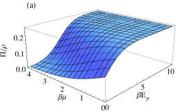
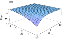
Figure 1: The unintegrated polarization per particle defined in Eq. (51) for fermions (a) and anti-fermions (b) at momentum $\mathbf{p}$ in the unit of the local vorticity $\hbar\boldsymbol{\omega}$ as functions of $\beta E_{p}$ and $\beta\mu$.

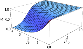
Figure 2: The ratio $R$ of polarization per particle in Eq. (55) for fermions to anti-fermions as a function of $\beta E_{p}$ and $\beta\mu$.

The numerical results for the unintegrated polarization per particle in Eq. (51) in the unit of the local vorticity $\hbar\boldsymbol{\omega}$ are shown in Fig. 1 in the range $\beta E_{p}=[0,10]$ and $\beta\mu=[0,4]$. At fixed values of energy $\beta E_{p}$, we see that $\boldsymbol{\Pi}(x,\mathbf{p})/\rho(x,\mathbf{p})$ is a decreasing (increasing) function of $\beta\mu$ for fermions (anti-fermions), but it always increases with $\beta E_{p}$ at fixed $\beta\mu$ for both fermions and anti-fermions. The numerical results for the ratio of $\boldsymbol{\Pi}(x,\mathbf{p})/\rho(x,\mathbf{p})$ for fermions to anti-fermions,

$$R=\frac{[\boldsymbol{\Pi}(x,\mathbf{p})/\rho(x,\mathbf{p})]_{\mathrm{fermion}}}{[\boldsymbol{\Pi}(x,\mathbf{p})/\rho(x,\mathbf{p})]_{\mathrm{anti-fermion}}},$$ (55)

are shown in Fig. 2. We see that $\boldsymbol{\Pi}(x,\mathbf{p})/\rho(x,\mathbf{p})$ for fermions is always less than that for anti-fermions, i.e. $R<1$, and $R$ decreases with $\beta\mu$ and increases with $\beta E_{p}$. When $\beta E_{p}$ is very large, the Fermi-Dirac distributions become Boltzmann ones and $\boldsymbol{\Pi}(x,\mathbf{p})/\rho(x,\mathbf{p})$ reaches its asymptotic value 1/4 (in the unit of $\hbar\boldsymbol{\omega}$) for both fermions and anti-fermions, which leads to $R\rightarrow 1$.

The numerical results for the integrated polarization per particle $\boldsymbol{\Pi}(x)/\rho(x)$ for fermions (left panel) and anti-fermions (right panel) are shown in Fig. 3 as functions of $\beta m$ and $\beta\mu$. The numerical results for the ratio of $\boldsymbol{\Pi}(x)/\rho(x)$,

$$R=\frac{[\boldsymbol{\Pi}(x)/\rho(x)]_{\mathrm{fermion}}}{[\boldsymbol{\Pi}(x)/\rho(x)]_{\mathrm{anti-fermion}}},$$ (56)

are shown in Fig. 4. In the left panel we show $R$ as a function of $\beta m$ and $\beta\mu$, while in the right panel we show $R$ at three values of $\beta\mu$ as functions of $\beta m$. The dependences of $\boldsymbol{\Pi}(x)/\rho(x)$ on $\beta m$ and $\beta\mu$ are similar to $\boldsymbol{\Pi}(x,\mathbf{p})/\rho(x,\mathbf{p})$ on $\beta E_{p}$ and $\beta\mu$, but the variation in the values of $\boldsymbol{\Pi}(x)/\rho(x)$ on $\beta m$ is much smaller than $\boldsymbol{\Pi}(x,\mathbf{p})/\rho(x,\mathbf{p})$ as shown in Figs. 1 and 2.

We see that $R<1$, i.e. the polarization per particle for fermions is always less than that for anti-fermions. This behavior is consistent to the observation in the STAR experiment Lisa (2016). Also $R$ decreases with $\mu$ at fixed $m$. Such behaviors are based on the following facts: (a) $\boldsymbol{\Pi}(x)$ is actually proportional to the susceptibility $\partial\rho/\partial\mu$ and increases/decreases for fermions/anti-fermions with $\beta\mu$ just as $\rho(x)$; (b) $\boldsymbol{\Pi}_{\mathrm{fermion}}/\boldsymbol{\Pi}_{\mathrm{anti-fermion}}$ and $\rho_{\mathrm{fermion}}/\rho_{\mathrm{anti-fermion}}$ are all increasing functions of $\beta\mu$; (c) $\boldsymbol{\Pi}_{\mathrm{fermion}}/\boldsymbol{\Pi}_{\mathrm{anti-fermion}}$ is less than $\rho_{\mathrm{fermion}}/\rho_{\mathrm{anti-fermion}}$ and increases slower with $\beta\mu$ than $\rho_{\mathrm{fermion}}/\rho_{\mathrm{anti-fermion}}$.

In the massless case, the momentum integrals in Eqs. (49,50) can be worked out, so we obtain the quantities for fermions ($+$) and anti-fermions ($-$),

$$\boldsymbol{\Pi}_{m=0}(x) = -\hbar\boldsymbol{\omega}\frac{1}{2\pi^{2}}\mathrm{Li}_{2}(-e^{\pm\beta\mu}),$$

$$\rho_{m=0}(x) = -\frac{2}{\pi^{2}}\mathrm{Li}_{3}(-e^{\pm\beta\mu}),$$

$$\left[\frac{\boldsymbol{\Pi}(x)}{\rho(x)}\right]_{m=0} = \hbar\boldsymbol{\omega}\frac{1}{4}\frac{\mathrm{Li}_{2}(-e^{\pm\beta\mu})}{\mathrm{Li}_{3}(-e^{\pm\beta\mu})},$$ (57)

where the polylogarithm function is defined by the power series, $\mathrm{Li}_{s}(z)=\sum_{k=1}^{\infty}z^{k}/k^{s}$. Fig. 5 shows the numerical results for $[\boldsymbol{\Pi}(x)/\rho(x)]_{m=0}$ for fermions and anti-fermions and their ratio $R$ defined by Eq. (56) as functions of $\beta\mu$.

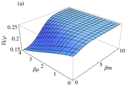
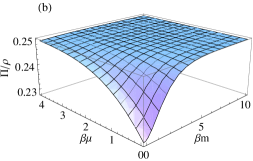
Figure 3: The integrated polarization per particle $\boldsymbol{\Pi}(x)/\rho(x)$ for fermions (a) and anti-fermions (b) in the unit of the local vorticity $\hbar\boldsymbol{\omega}$ as functions of $\beta m$ and $\beta\mu$.

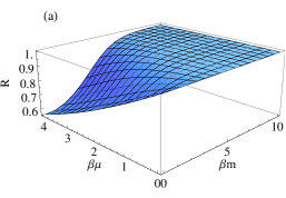
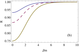
Figure 4: The ratio $R$ of the integrated polarization per particle in Eq. (56) for fermions to anti-fermions. (a) $R$ as a function of $\beta m$ and $\beta\mu$. (b) $R$ as functions of $\beta m$ at three values $\beta\mu=0.5,\,1,\,2$ corresponding to short-dashed, long-dashed and solid lines respectively.

   

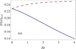
Figure 5: (a) The integrated polarization per particle $\boldsymbol{\Pi}(x)/\rho$ for massless fermions (solid line) and anti-fermions (long-dashed line) in the unit of $\hbar\boldsymbol{\omega}$ as functions of $\beta\mu$. (b) The ratio $R$ of the integrated polarization per particle in Eq. (56) for fermions to anti-fermions as a function of $\beta\mu$.

If we consider the Cooper-Frye description of hadron freezeout in hydrodynamic evolution, we can re-write the polarization density in Eq. (47) by replacing the momentum integral with the one on the freezeout hypersurface. For fermions, we pick up the first term in the second line of Eq. (47) and define the polarization spectra in momentum space as,

$$\frac{d\Pi^{\alpha}(p)}{d^{3}p} \approx \frac{\hbar}{2mE_{p}}\int d\Sigma_{\lambda}p^{\lambda}\tilde{\Omega}^{\alpha\sigma}p_{\sigma}f_{\mathrm{FD}}(x,p)(1-f_{\mathrm{FD}}(x,p)),$$ (58)

where $p^{\mu}$ denote the on-shell 4-momentum and we have $p^{\mu}=(E_{p},\mathbf{p})$ in the co-moving frame. The particle number distribution for fermions is given by

$$f_{\mathrm{FD}}(x,p)=\frac{1}{e^{\beta(x)[u(x)\cdot p-\mu]}+1}.$$ (59)

In Eq. (58), we note that $\Pi^{\alpha}(p)$ is the polarization of fermions with the momentum $p$ and has the unit $\hbar$. We can verify that the Lorentz transformation rule for both sides of Eq. (58) are the same. The particle number spectra for fermions in momentum space emitting on the freezeout hypersurface can be defined as

$$\frac{d\rho(p)}{d^{3}p}=\frac{2}{E_{p}}\int d\Sigma_{\lambda}p^{\lambda}f_{\mathrm{FD}}(x,p),$$ (60)

where the factor 2 is from two spin orientations. Then we obtain the polarization per particle for fermions with the momentum $p$,

$$\mathscr{P}^{\alpha}(p)\equiv\frac{d\Pi^{\alpha}(p)/d^{3}p}{d\rho(p)/d^{3}p} = \frac{\hbar}{4m}\frac{\int d\Sigma_{\lambda}p^{\lambda}\tilde{\Omega}^{\alpha\sigma}p_{\sigma}\,f_{\mathrm{FD}}(x,p)[1-f_{\mathrm{FD}}(x,p)]}{\int d\Sigma_{\lambda}p^{\lambda}\,f_{\mathrm{FD}}(x,p)}.$$ (61)

Eq. (61) is a covariant expression for the polarization vector per particle which is the same as the result by Becattini et al Becattini et al. (2013b). For anti-fermions, we can flip the sign of the chemical potential, $\mu\rightarrow-\mu$, in the above formula. We see from Eq. (47) that the total polarization is the sum of fermion and anti-fermion contributions.

VII Summary and conclusion

We have extended our previous works on the Wigner function for chiral or massless fermions to that for massive fermions. The Wigner function at the leading order is derived from its definition by setting the gauge link to 1 and by expanding the free form of the fermionic quantum fields in momentum space. Then all components of the Wigner function can be extracted by projecting the corresponding Dirac matrices and taking traces. The axial vector component at the next-to-leading order for massive fermions can be obtained by extending that for massless fermions and satisfies the required equations. We have shown that the axial vector component behaves like a spin 4-vector in phase space up to a factor 1/2. The polarization density can be computed by integration of the axial vector component over momentum. Our numerical results show that the polarization per particle decreases/increases with the (temperature normalized) chemical potential for fermions/anti-fermions at fixed (temperature normalized) energy (mass), while it always increases with the (temperature normalized) energy (mass) at fixed (temperature normalized) chemical potential. We have found that the polarization per particle for fermions is always less than that for anti-fermions. At large energy (mass) limit the polarization per particle approaches the asymptotic value $\hbar\boldsymbol{\omega}/4$ for both fermions and anti-fermions following the Boltzmann distribution. We have also formulated the polarization per particle for fermions with the specific momentum on the Cooper-Frye freezeout hypersurface in a hydrodynamic description, which is consistent to the previous result of Becattini et al..

Acknowledgments. QW is supported in part by the Major State Basic Research Development Program (MSBRD) in China under the Grant No. 2015CB856902 and 2014CB845406 and by the National Natural Science Foundation of China (NSFC) under the Grant No. 11535012. XNW is supported in part by the National Natural Science Foundation of China (NSFC) under the Grant No. 11221504 and by the Chinese Ministry of Science and Technology under Grant No. 2014DFG02050, and by the Director, Office of Energy Research, Office of High Energy and Nuclear Physics, Division of Nuclear Physics, of the U.S. Department of Energy under Contract No. DE- AC02-05CH11231. LGP is supported in part by Helmholtz Young Investigator Group VH-NG-822 from the Helmholtz Association and GSI.

References

Liang and Wang (2005a)
Z.-T. Liang and
X.-N. Wang,
Phys. Rev. Lett. 94,
102301 (2005a),
[Erratum: Phys. Rev. Lett.96,039901(2006)],
eprint nucl-th/0410079.
Liang and Wang (2005b)
Z.-T. Liang and
X.-N. Wang,
Phys. Lett. B629,
20 (2005b),
eprint nucl-th/0411101.
Becattini et al. (2008)
F. Becattini,
F. Piccinini,
and J. Rizzo,
Phys. Rev. C77,
024906 (2008), eprint 0711.1253.
Betz et al. (2007)
B. Betz,
M. Gyulassy, and
G. Torrieri,
Phys. Rev. C76,
044901 (2007), eprint 0708.0035.
Huang et al. (2011)
X.-G. Huang,
P. Huovinen, and
X.-N. Wang,
Phys. Rev. C84,
054910 (2011), eprint 1108.5649.
Jiang et al. (2016)
Y. Jiang,
Z.-W. Lin, and
J. Liao
(2016), eprint 1602.06580.
Deng and Huang (2016)
W.-T. Deng and
X.-G. Huang
(2016), eprint 1603.06117.
Csernai et al. (2011)
L. P. Csernai,
V. K. Magas,
H. Stocker, and
D. D. Strottman,
Phys. Rev. C84,
024914 (2011), eprint 1101.3451.
Wang et al. (2013)
D. J. Wang,
Z. Neda, and
L. P. Csernai,
Phys. Rev. C87,
024908 (2013), eprint 1302.1691.
Becattini
et al. (2013a)
F. Becattini,
L. Csernai, and
D. J. Wang,
Phys. Rev. C88,
034905 (2013a),
eprint 1304.4427.
Abelev et al. (2007)
B. I. Abelev
et al. (STAR), Phys.
Rev. C76, 024915
(2007), eprint 0705.1691.
Deng (2014)
J. Deng, Phys.
Part. Nucl. 45, 73
(2014).
Kharzeev et al. (2008)
D. E. Kharzeev,
L. D. McLerran,
and H. J.
Warringa, Nucl.Phys.
A803, 227 (2008),
eprint 0711.0950.
Fukushima et al. (2008)
K. Fukushima,
D. E. Kharzeev,
and H. J.
Warringa, Phys.Rev.
D78, 074033
(2008), eprint 0808.3382.
Son and Surowka (2009)
D. T. Son and
P. Surowka,
Phys.Rev.Lett. 103,
191601 (2009), eprint 0906.5044.
Kharzeev and Son (2011)
D. E. Kharzeev and
D. T. Son,
Phys.Rev.Lett. 106,
062301 (2011), eprint 1010.0038.
Pu et al. (2011)
S. Pu,
J.-h. Gao, and
Q. Wang,
Phys. Rev. D83,
094017 (2011), eprint 1008.2418.
Gao et al. (2012)
J.-H. Gao,
Z.-T. Liang,
S. Pu,
Q. Wang, and
X.-N. Wang,
Phys.Rev.Lett. 109,
232301 (2012), eprint 1203.0725.
Gao and Wang (2015)
J.-h. Gao and
Q. Wang,
Phys. Lett. B749,
542 (2015), eprint 1504.07334.
Elze et al. (1986)
H.-T. Elze,
M. Gyulassy, and
D. Vasak,
Nucl.Phys. B276,
706 (1986).
Vasak et al. (1987)
D. Vasak,
M. Gyulassy, and
H.-T. Elze,
Annals Phys. 173,
462 (1987).
Chen et al. (2013)
J.-W. Chen,
S. Pu,
Q. Wang, and
X.-N. Wang,
Phys.Rev.Lett. 110,
262301 (2013), eprint 1210.8312.
Zhuang and Heinz (1996)
P. Zhuang and
U. W. Heinz,
Annals Phys. 245,
311 (1996), eprint nucl-th/9502034.
Ochs and Heinz (1998)
S. Ochs and
U. W. Heinz,
Annals Phys. 266,
351 (1998), eprint hep-th/9806118.
Lisa (2016)
M. Lisa,
Preliminary results by STAR, on the Workshop on Chirality,
Vorticity and Magnetic Field in Heavy Ion Collisions, Los Angeles, February
23-26, 2016 (2016).
Becattini
et al. (2013b)
F. Becattini,
V. Chandra,
L. Del Zanna,
and E. Grossi,
Annals Phys. 338,
32 (2013b), eprint 1303.3431.