Boxy H$\alpha$ Emission Profiles in Star-Forming Galaxies

Abstract

We assemble a sample of disk star-forming galaxies from the Sloan Digital Sky Survey Data Release 7, studying the structure of H$\alpha$ emission lines, finding a large fraction of this sample contains boxy H$\alpha$ line profiles. This fraction depends on galaxy physical and geometric parameters in the following way: (1) it increases monotonically with star formation rate per unit area ($\Sigma_{\rm SFR}$), and stellar mass ($M_{*}$), with the trend being much stronger with $M_{*}$, from $\sim$0% at $M_{*}=10^{10}M_{\odot}$ to about 50% at $M_{*}=10^{11}M_{\odot}$; (2) the fraction is much smaller in face-on systems than in edge-on systems. It increases with galaxy inclination ($i$) while $i<60\,^{\circ}$ and is roughly a constant of 25% beyond this range; (3) for the sources which can be modeled well with two velocity components, blueshifted and redshifted from the systemic velocity, these is a positive correlation between the velocity difference of these two components and the stellar mass, with a slope similar to the Tully-Fisher relation; (4) the two components are very symmetric in the mean, both in velocity and in amplitude. The four findings listed above can be understood as a natural result of a rotating galaxy disk with a kpc-scale ring-like H$\alpha$ emission region.

1 Introduction

Over the last decade, a huge amount of effort has been expended mapping the evolution of the star formation rate (SFR) density of the universe with time and stellar mass (e.g., Brinchmann et al., 2004; Bauer et al., 2005; Feulner et al., 2005; Noeske et al., 2007; Zheng et al., 2007; Chen et al., 2009). The H$\alpha$, [O ii] , ultraviolet-optical spectral energy distribution (SED) fitting and infrared photometry are commonly used to estimate the SFR at different redshifts. Two major conclusions of these studies are (1) the comoving SFR density of the universe has declined by an order of magnitude since $z\sim 2$ (Hopkins et al., 2006); (2) the SFR per unit stellar mass (SSFR) depends on both stellar mass and redshift, with massive galaxies forming most of their stars earlier than less massive systems (Heavens et al., 2004; Thomas et al., 2005).

To fully understand galaxy formation and evolution, it is important to understand both how the population as a whole evolves and how SFR within individual galaxies evolves. A first step is looking at how SFR is distributed spatially in galaxies as a function of their physical parameters, such as stellar mass and environment. However this is not an easy task, especially for high$-z$ galaxies given their small angular size and faintness. The radial distribution of star formation in local galaxies has been analysed in individual galaxies (e.g. NGC1566, Comte & Duquennoy, 1982) and samples of tens to hundreds of galaxies using narrow band imaging centered on H$\alpha$ which traces the ionizing photons produced by massive stars. Ryder & Dopita (1994) studied the relative scale lengths of H$\alpha$, $V-$ and $I-$ band emission in 34 S0-Sm galaxies, finding that the line emission had a larger scale length than the continuum. James et al. (2009) compared the H$\alpha$ and $R$-band light profiles of 313 S0a-Im field galaxies, finding the major central H$\alpha$ deficit (relative to the continuum) happens in barred galaxies, particularly in early-type and hence high mass barred galaxies (see also Hakobyan et al., 2014; Nair & Abraham, 2010). Statistical studies of larger volumes have so far been lacking due to the decrease in spatial resolution with distance, and the necessity of using multiple narrow band filters to accommodate the redshifting of the H$\alpha$ line.

Sloan Digital Sky Survey provides the largest galaxy sample of photometry and spectra so far. It is a great database to study all kinds of properties of local galaxies. Ge et al. (2012) select double-peaked narrow emission-line galaxy sample from SDSS DR7 and study their properties. However, due to the 3” diameter fiber, it is hard to derive any spatial information about the galaxies directly from the spectra. In this paper, we make the first attempt of getting spatial information from the structures of H$\alpha$ emission lines in SDSS spectra. As we know, the H$\alpha$ profile depends on the strength of emission at a given velocity, which is determined by the rotating curve and the H$\alpha$ surface brightness distribution in a rotating disk. Thus through comparing observed H$\alpha$ line structures with the simulated H$\alpha$ line profiles for the rotating disk model, we can have an idea of the possible distribution of the H$\alpha$ surface brightness. In §2, we introduce the sample selection criteria used in our study. We characterize the H$\alpha$ emission line profiles and study the relation between line profiles and galaxy physical/geometric parameters in §3. The origin of the boxy line profile (please see §3.1 for the definition of peakiness or boxiness of a line) is found to be a rotating disk with a kpc-scale ring-like H$\alpha$ emission region in §4. The results are summarized in §5.

2 Sample and Data Analysis

2.1 The Data

The seventh data release (DR7; Abazajian et al., 2009) of Sloan Digital Sky Survey (SDSS; York et al., 2000) contains $\sim$930,000 galaxy spectra. The spectra are taken through $3^{\prime\prime}$ diameter fibers with a dispersion of 69 km s^-1 pixel^-1. These galaxies cover a redshift range of $z=0-0.3$. In this work, we analyze objects drawn from the “Main” galaxy sample (Strauss et al., 2002) which are selected to have Petrosian magnitudes in the range $14.5<r<17.7$ after correction for foreground Galactic extinction using the reddening maps of Schlegel et al. (1998).

The stellar continuum is fitted with stellar population models (Tremonti et al., 2004; Brinchmann et al., 2004). The basic assumption of this fitting is that any galaxy star formation history can be approximated as a sum of discrete bursts. The library of template spectra is composed of single stellar population (SSP) models generated using a preliminary version of the population synthesis code of Charlot & Bruzual (in prep., hereafter CB08). We refer the reader to Tremonti et al. (2004) for more details about the fitting process. The results of this fitting procedure and measurements of a number of line indices (e.g., D4000, H$\delta_{A}$) can be found in the MPA/JHU catalogue.

We use our best fit stellar continuum model to re-measure each galaxy’s redshift using a cross correlation technique and masking out regions of the data with emission lines. These redshifts differ very slightly from the SDSS pipeline redshifts which use cross correlation templates that include emission lines. The new redshifts enable us to accurately measure the gas motions with respect to the stars.

The derived galaxy parameters required in this work include stellar mass ($M_{*}$), star formation surface density ($\Sigma_{\rm SFR}$), and galaxy inclination ($i$). The stellar masses are estimated from the $ugriz$ colors of the galaxies. Connecting these colors with a large grid of CB08 model colors following the methodology described in Salim et al. (2007), the maximum likelihood estimate of the $z$-band mass-to-light ratio for a galaxy can be obtained. We derive SFRs from the dust extinction corrected H$\alpha$ luminosity using the formula of Kennicutt (1998), converting from a Salpeter to Kroupa initial mass function (Kroupa, 2001) by dividing by a factor of 1.5. $\Sigma_{\rm SFR}$ is defined as SFR/$\pi R^{2}$, where $R$ is the $1.5^{\prime\prime}$ fiber radius of SDSS corrected for projection effects. We use $\Sigma_{\rm SFR}$ instead of SFR because the former is less subject to aperture bias.

The SDSS photometric pipeline (Lupton et al., 2001) fits a two-dimensional model of an exponential profile and a de Vaucouleurs (1948) profile to each galaxy image. The best linear combination of the exponential and de Vaucouleurs models is stored in a parameter called $\rm fracDeV$ (Abazajian et al., 2004). An axial ratio ($b/a$) is given by this fitting procedure. Here we use $\rm fracDeV$ to distinguish disk galaxies (${\rm fracDeV}<0.8$) from early-type galaxies (${\rm fracDeV}\geq 0.8$) (Padilla & Strauss, 2008). The axis ratios from the exponential and de Vaucouleurs models are consistent with each other. The inclinations of disk galaxies are computed from the measured axial ratio, $b/a$, and the $r-$band absolute magnitude $M_{\rm r}$ using Table 8 in Padilla & Strauss (2008).

2.2 Sample Selection

The sample is selected by the following criteria:

1. redshift of $\rm 0.1\leq z\leq 0.15$. We limit our sample to this small redshift range to ensure that we are sampling the same physical scale of the galaxies. With $3^{\prime\prime}$ diameter fibers, the SDSS spectra probe the central 5–7 kpc in this redshift range.

2. $r-$band $\rm fracDeV<0.8$. This criterion selects disk galaxies, which makes the calculation of the inclination angle from $b/a$ possible.

3. $\log(\Sigma_{\rm SFR})>-0.15$. This criterion selects galaxies that are forming stars. Combined with our redshift cut, it also insures that the H$\alpha$ lines are measured with reasonable signal-to-noise (S/N).

4. $\log($[O iii] /H$\beta)<0.61/\{\log($[N ii] /H$\alpha)-0.05\}+1.3$. Only star forming galaxies are included in our sample (Kauffmann et al., 2003).

We refer to this sample hereafter as our parent sample. It contains 18,425 galaxies.

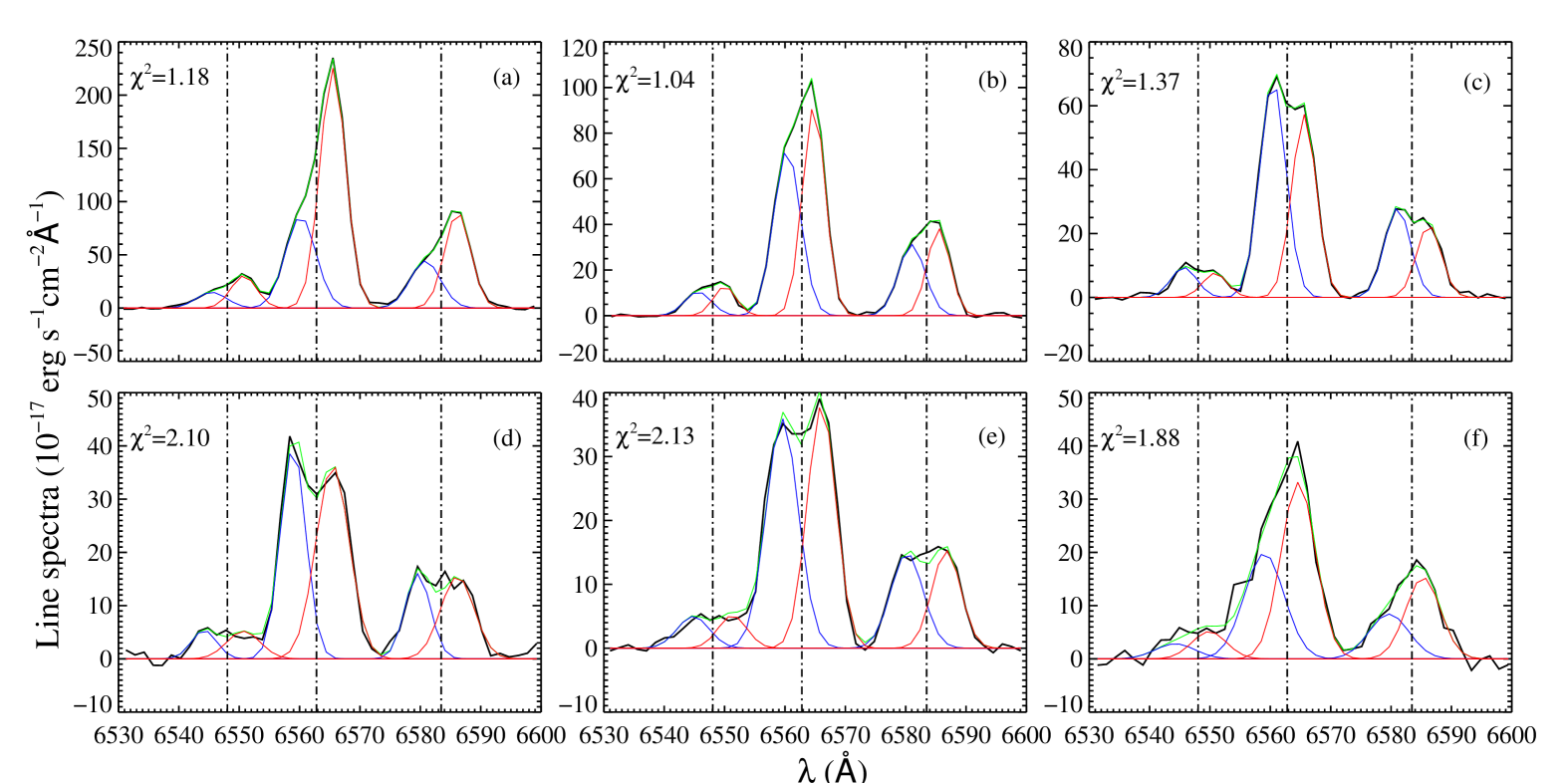
Figure 1: Examples of boxy H$\alpha$ and [N ii] emission. The data is shown in black; blue and red lines show Gaussian fits to the blueshifted and redshifted emission components; the green lines show the combined fits. The dashed vertical lines mark the restframe wavelength of the [N ii] $\lambda$6548, H$\alpha$ $\lambda$6563, [N ii] $\lambda$6583 emission lines. The top panel shows cases that can be modeled well with two Gaussian components; the bottom panel shows failed fits due to complicated line structures. The reduced $\chi^{2}$ is given in the top-left corner of each panel.

3 H$\alpha$ Emission Line Profiles

3.1 Characterizing Emission Line Profiles

We calculate the fourth moment or kurtosis of the H$\alpha$ emission lines (hereafter ${\rm H}\alpha_{\rm kur}$) from the continuum-subtracted spectrum. The kurtosis characterizes the peakiness or boxiness of a line. For a gaussian profile, we would expect a ${\rm H}\alpha_{\rm kur}=3$, with boxier profiles yielding smaller values of kurtosis. We find that sources with ${\rm H}\alpha_{\rm kur}<2.4$ contain more than one velocity component.

We also explore parametric fits to the line profiles. We use six gaussian components to fit the H$\alpha$ and [N ii] $\lambda$6548,6584 lines simultaneously, with two components for each line. Each [N ii] $\lambda$6548 component is forced to have the same centroid and width as the corresponding [N ii] $\lambda$6583 component, and the flux ratio of [N ii] $\lambda$6583 to [N ii] $\lambda$6548 is fixed to be 3. The top panel of Figure 1 shows three typical examples of our fits. In some cases, the H$\alpha$ lines can be fitted well with two gaussian components, one blueshifted and the other redshifted relative to the systemic velocity defined by the stars. There are other cases in which two gaussian components cannot model the line profile due to the complicated structure of H$\alpha$ (see the buttom panel). The reduced $\chi^{2}$ is given in the top-left corner of each panel.

For comparison, we visually inspect all the emission line spectra and try to select sources with boxy H$\alpha$ emission by eye. In this sample we only include objects which clearly contain more than one velocity component in both the H$\alpha$ and [N ii] lines and we require the components to be blueshifted and redshifted relative to the systemic velocity. We do not include galaxies that exhibit low-level wings on their line profiles. As we will show in §3.2, we find good agreement between our visually identifed sample and galaxies with ${\rm H}\alpha_{\rm kur}<2.4$. We refer to the 2815 sources with ${\rm H}\alpha_{\rm kur}<2.4$ as “boxy sources” hereafter.

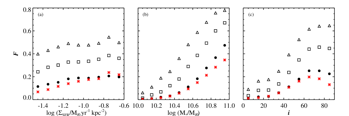
Figure 2: The fraction of boxy sources vs. star formation surface density, $\Sigma_{\rm SFR}$, stellar mass, $M_{*}$, and galaxy inclination, $i$. The black points indicate the fraction of galaxies with H$\alpha$ kurtosis below a certain threshold. For reference, a Gaussian line profile has ${\rm H}\alpha_{\rm kur}=3$; smaller values indicate increasing boxiness. The triangles, squares and solid dots show $F=N({\rm H}\alpha_{\rm kur}<2.7)/N_{\rm bin}$, $F=N({\rm H}\alpha_{\rm kur}<2.55)/N_{\rm bin}$ and $F=N({\rm H}\alpha_{\rm kur}<2.4)/N_{\rm bin}$, respectively. $N({\rm H}\alpha_{\rm kur}<2.4)$ is the number of galaxies with ${\rm H}\alpha_{\rm kur}$ smaller than $2.4$ in a given galaxy parameter bin and $N_{\rm bin}$ is the total number of galaxies in the bin. Red asterisks show the fraction of galaxies visually identified as having two velocity components.

3.2 The Fraction of Galaxies with Boxy H$\alpha$ Emission Profiles

In this section, we examine how the boxy source fraction varies as a function of galaxy physical and geometrical properties: $\Sigma_{\rm SFR}$, $M_{*}$, and $i$.

We divide our parent sample into bins in $\Sigma_{\rm SFR}$, $M_{*}$, and $i$. In each bin we measure the fraction, $F$, of galaxies with H$\alpha$ kurtosis below a given theshold, for example, $F=N({\rm H}\alpha_{\rm kur}<2.4)/N_{\rm bin}$. Here $N({\rm H}\alpha_{\rm kur}<2.4)$ is the number of galaxies with ${\rm H}\alpha_{\rm kur}$ smaller than $2.4$ in a given bin and $N_{\rm bin}$ is the total number of galaxies in the bin. In Figure 2 we show how the fraction of galaxies with boxy H$\alpha$ profiles varies with galaxy physical parameters. The black symbols show the fraction of galaxies in each bin with ${\rm H}\alpha_{\rm kur}$ less than 2.6, 2.55, and 2.4 (triangles, squares, and circles) and the red asterisks show the fraction of galaxies in each bin visually identified as having two velocity components. The trends between $F$ and galaxy parameters are very similar for the different ${\rm H}\alpha_{\rm kur}$ theresholds, with the main differenence being in the absolute value of $F$. The results from our visual inspection agree closely with galaxies with ${\rm H}\alpha_{\rm kur}<2.4$ (solid circles). This suggests that our kurtosis measurements are very effective at selecting galaxies with boxy H$\alpha$ profiles and that our results are independent of the exact ${\rm H}\alpha_{\rm kur}$ threshold adopted.

Figure 2$a$ and $b$ show that the fraction of galaxies with boxy H$\alpha$ lines increases monotonically with both $\Sigma_{\rm SFR}$ and $M_{*}$. The fraction increases more dramatically with stellar mass, from $\sim$0% at $M_{*}=10^{10}M_{\odot}$ to about 50% at $M_{*}=10^{11}M_{\odot}$ for the subsample with the highest degree of boxiness (${\rm H}\alpha_{\rm kur}<2.4$). Figure 2c shows that the boxy fraction increases rapidly with inclination while $i<60\,^{\circ}$. Above this value it is roughly constant at $F\sim$25% for the galaxies with the highest degree of boxiness.

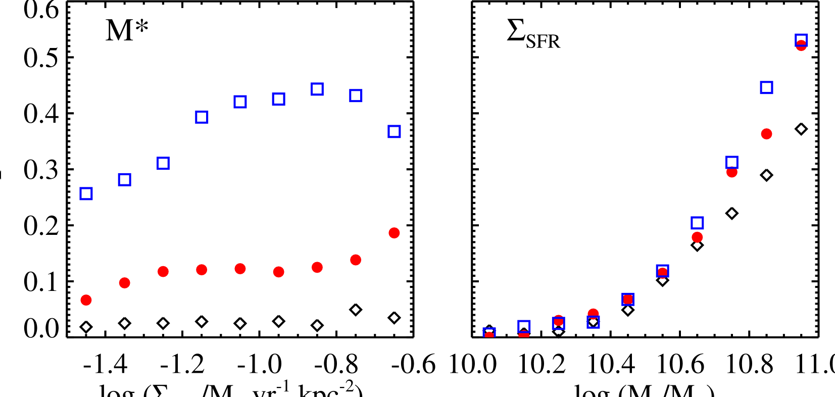
Figure 3: The dependence of the boxy source fraction on $\Sigma_{\rm SFR}$ and $M_{*}$. In each panel, the sample is divided into three sub-bins by the parameter marked in the top-left corner. The black, red, and blue points indicate the low, median, and high sub-bins respectively. This approach is designed to help mitigate the effect of $M_{*}-\Sigma_{\rm SFR}$ correlation. The physical parameters that play the dominant role in driving the trends will show the smallest offsets between the black, red, and blue points.

Figure  2 shows that the boxy source fraction depends more strongly on $M_{*}$ than on $\Sigma_{\rm SFR}$. However, due to the correlation between $\Sigma_{\rm SFR}$ and $M_{*}$ for star forming disk galaxies (see Figure 1 of Chen et al. 2010), it is difficult to figure out whether $\Sigma_{\rm SFR}$ is a real driver of boxy line profiles or whether the trend between $F$ and $\Sigma_{\rm SFR}$ is just an inevitable by-product of the $F-M_{*}$ relation. To solve this problem, we split $\Sigma_{\rm SFR}$ into different bins and take each bin in $\Sigma_{\rm SFR}$ and futher divide it into three equal sub-bins, sorting the galaxies by $M_{*}$. We are then able to study the trends between $F$ and $\Sigma_{\rm SFR}$ in low, median and high $M_{*}$ bins (where the exact division between low, median and high changes with $\Sigma_{\rm SFR}$). If $\Sigma_{\rm SFR}$ is the most important parameter in driving the boxy line profiles, then very little difference is expected between the sub-bins in $M_{*}$ and fixed $\Sigma_{\rm SFR}$. Conversely, if $M_{*}$ is the dominant driver, the three sub-bins will be strongly offset from one another at each value of $\Sigma_{\rm SFR}$.

Figure 3 shows the fraction of boxy sources ($F=N({\rm H}\alpha_{\rm kur}<2.4)/N_{\rm bin}$) as a function of $\Sigma_{\rm SFR}$ and $M_{*}$. In each panel the sample is split into three sub-bins according to the galaxy parameter labeled in the top-left corner. The black, red, and blue points indicate the low, median and high sub-bins respectively. Figure 3 adds to the evidence that $M_{*}$ is the dominant driver of the boxy line profiles and proves that the $F-\Sigma_{\rm SFR}$ relation shown in Figure 2 is a by-product of $F-M_{*}$ and $M_{*}-\Sigma_{\rm SFR}$ correlation. The $F-M_{*}$ trend appears to be totally independent of $\Sigma_{\rm SFR}$ at low masses, with a very weak trend evident at $M_{*}>10^{10.7}M_{\odot}$.

4 The Origin of Boxy H$\alpha$ Profiles

Having established that boxy H$\alpha$ profiles are common in massive edge on disk galaxies in the SDSS, we now turn to the question of their origin.

4.1 Bi-polar Outflows

H$\alpha$ emission line profiles have been studied in detail in several nearby starburst galaxies using longslit spectra or narrow band images (e.g., Heckman et al., 1990; Lehnert & Heckman, 1996; Greve et al., 2000; Westmoquette et al., 2009). The purpose of these works was to search for evidence of stellar wind/supernova driven outflows and to constrain their geometry and dynamics. In these works, double-peaked H$\alpha$ emission-line profiles (one special case of boxy structure) were commonly found in minor axis spectra. This was explained as a combination of the emission from both the near side and far side of one outflow cone.

An SDSS fiber spectrum samples the central $3^{\prime\prime}$ of a galaxy which corresponds to radii of 2.5 – 3.5 kpc for our sample. This aperature could encompass the emission from both the disk and two outflow bi-cones if they exist. However, it should be kept in mind that the emission from the outflow is expected to be very weak relative to the disk. Lehnert et al. (1999) looked at H$\alpha$ emission in the starburst galaxy M82 and found that the wind contributes only $\sim 0.3$% of the total flux. The other arguement against the outflow hypothesis is that the fraction of boxy sources correlates much more strongly with $M_{*}$ than $\Sigma_{\rm SFR}$. This is surprising because Chen et al. (2010) showed that the amount of cool gas in galactic winds in normal star forming galaxies is a strong function of $\Sigma_{\rm SFR}$. Thus we conclude that bi-polar galactic winds, while possibly present, are not responsible for the boxy H$\alpha$ line profiles we observe.

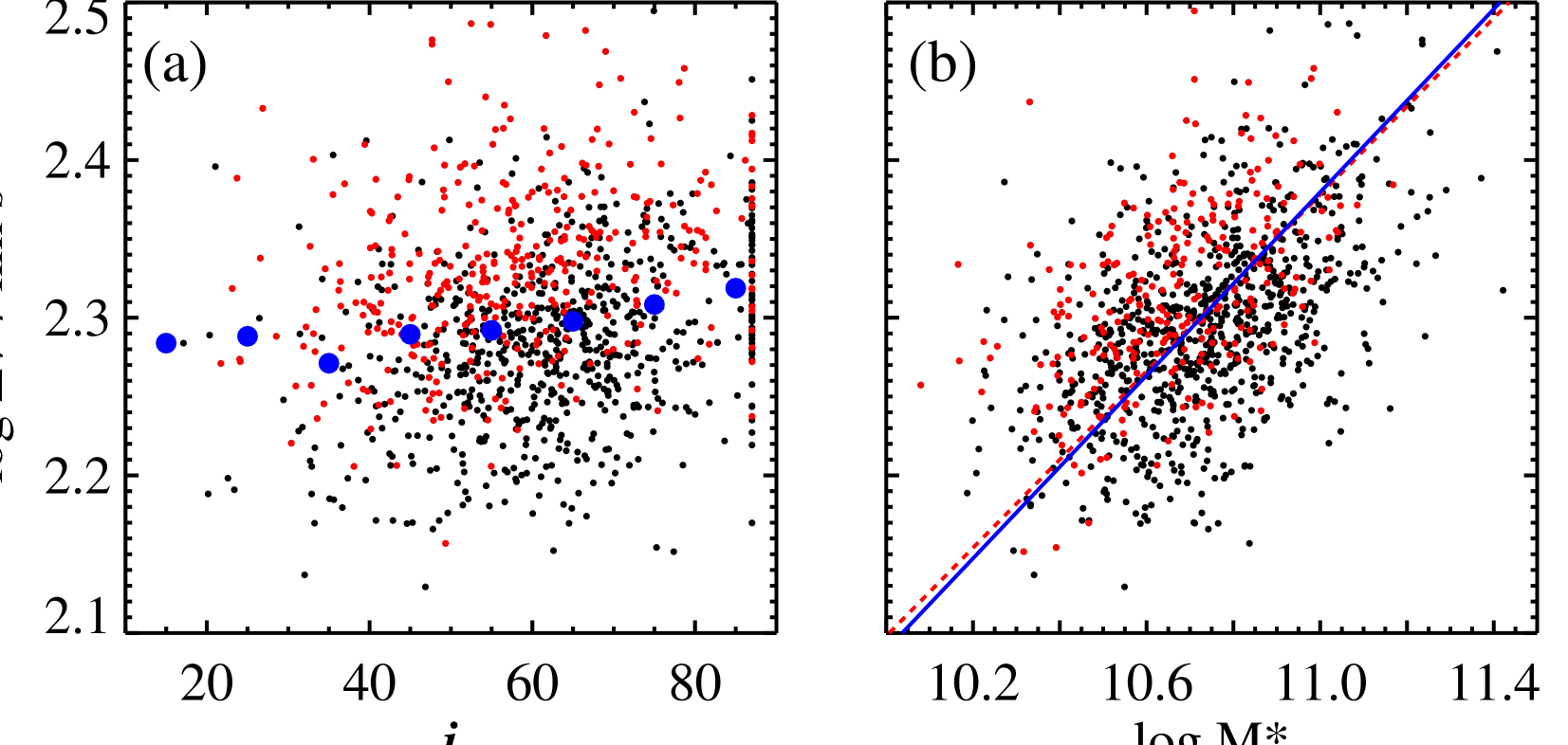
Figure 4: The dependence of $\Delta v$, the velocity difference between the two components, on inclination and stellar mass. The black dots show the data points. In the left panel, the blue dots are medians. In the right panel, the blue line is a linear regression of the data. The red dashed line has the same slope as the Tully-Fisher relation and an arbitrary intercept. The over-plotted red dots represent high mass ($M_{*}>10^{10.8}M_{\odot}$) and high inclination ($i>70\,^{\circ}$) sources in left and right panels respectively.

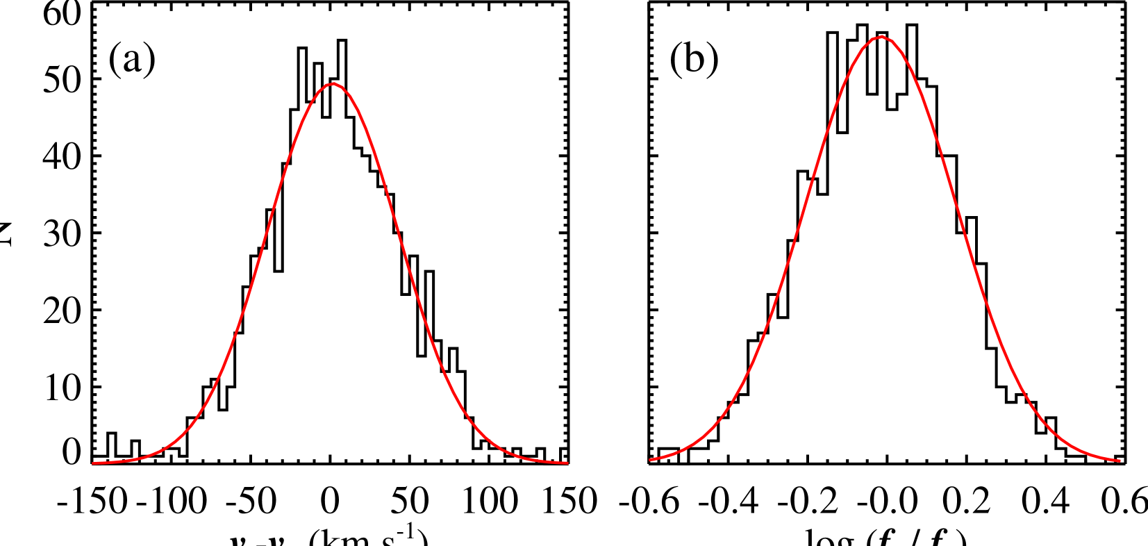
Figure 5: Histograms of the velocity difference ($v_{\rm r}-v_{\rm b}$; left panel) and flux ratios ($f_{\rm r}/f_{\rm b}$; right panel) between the blue-shifted and red-shifted emisison line components. The red curves show gaussian fits.

4.2 Star Formation in the Disk

The boxy H$\alpha$ line profiles may also be produced by star formation in the disk for certain H$\alpha$ surface brightness distributions. The simplest case is star forming disk with a central hole. In this scenario, the blueshifted and redshifted velocity peaks arise from gas in the ring moving directly towards and away from us. While the bi-polar outflow model encounters problems in explaining the trends between the boxy source fraction and galaxy physical parameters ($\Sigma_{\rm SFR}$ and $M_{*}$), these two relations can be naturally explained by the rotating disk model: the higher the stellar mass, the larger the rotational velocity of the disk, which would lead to larger velocity splitting and a higher detection rates of boxy sources.

The inclination dependence is also broadly consistent with our expectations for a disk. The velocity spread between the peaks will scale as sin($i$) and be maximum when the disk is edge on ($i=90^{\circ}$). At lower inclinations only the most massive galaxies with the largest intrinsic rotation speeds will be detected as boxy sources, hence the fall off in $F$ at low $i$. Above $i=60\,^{\circ}$ inclination effects change the velocity spread by less than 15%, so $F$ appears roughly constant. The small dip at $i\sim 90$ may be due to extinction effects in fully edge-on disks.

For the 1088 sources that can be modeled well with two velocity components, we examine how the velocity difference between the peak of the two gaussians ($\Delta v$) depends on galaxy inclination and stellar mass. Figure 4$a$ shows $\Delta v$ as a function of $i$, with blue dots indicating median values. At first sight, the lack of correlation in this plot conflicts with the prediction of the toy rotating disk model: $\Delta v\propto$ sin($i$). However, there is a strong selection effect at work: it is not possible to fit two well-separated gaussians to sources with $\Delta v$ below the SDSS resolution of 150 km s^-1. At fixed inclination we expect a range in mass and thus a range in $\Delta v$ down to the resolution limit. The over-plotted red dots in Figure 4$a$ show the subsample of high mass galaxies with $M_{*}>10^{10.8}M_{\odot}$, which is believed to suffer less selection effect.

Figure 4$b$ shows that $\Delta v$ increases with increasing $M_{*}$. The blue line shows a linear regression:

$$\log\Delta v=(0.29\pm 0.02)\log{M_{*}}-(0.81\pm 0.18)$$ (1)

The fit has a Pearson’s correlation coefficient of 0.53 and a probability of less than $10^{-5}$ that it could be obtained by chance. The red dashed line has the same slope as the Tully-Fisher relation (Tully & Fisher, 1977; Bell & de Jong, 2001) with an arbitrary value of the intercept. Since most of the objects in Figure  4$a$ have $i>50\,^{\circ}$, the effects of inclination on $\Delta v$ are small enough to be neglected in Figure 4$b$. The similarity of the slope of our $\Delta v$–$M_{*}$ relation and the Tully-Fisher relation is somewhat surprising considering that the SDSS fiber apertures do not necessarily sample out to the flat part of the rotation curve. Nevertheless, this consistency provides support for the rotating disk model as the dominant origin of the boxy line profiles found in our sample. We also over-plotted the high inclination sources ($i>70\,^{\circ}$) in Figure 4$b$ as red dots to show how the selection effect of inclination influences our result.

4.2.1 Further Tests of the Disk Hypothesis

The rotating disk model also predicts that the blueshifted and redshifted components should have roughly equal and opposite velocities relative to the systemic velocity of the stars ($v_{r}-v_{b}=0$ km s^-1). Moreover, while patchy extinction could result in one velocity component being stronger than the other in an individual galaxy, in the mean, the flux ratio of the two components should be unity ($f_{b}/f_{r}=1$). We test these two predictions in Figure 5. Figure 5$a$ shows a histogram of the velocity difference between the redshifted ($v_{\rm r}$) and blueshifted ($v_{\rm b}$) components. As expected, for the disk model, the distribution is strongly peaked about zero. Figure 5$b$ shows the distribution of flux ratios between the redshifted ($f_{\rm r}$) and blueshifted ($f_{\rm b}$) components. It is also very consistent with the expectations of the disk model.

4.3 Evidence for central kiloparsec-scale H$\alpha$ deficit region

4.3.1 Simple Models

Having demonstrated that the boxy H$\alpha$ emission line profiles arise from star formation in a rotating disk, we now turn to discussing the distribution of star formation. To do this we employ a simple toy model of a fully edge-on disk in solid body rotation out to 3 kpc and a flat rotation curve with $V_{C}$=200 km $s^{-1}$ at larger radii. The observed H$\alpha$ line profile depends on the strength of the emission at a given velocity. To determine this we consider various H$\alpha$ surface brightness distributions and add up the amount of emission at each velocity within 3 kpc (the SDSS aperture). The resulting H$\alpha$ line profile is then convolved to the SDSS spectral resolution of 150 km s^-1. For an exponential H$\alpha$ light distribution, the synthetic profile has ${\rm H}\alpha_{\rm kur}=2.55$, which is less peaked than a Gaussian (${\rm H}\alpha_{\rm kur}=3$) but considerably more peaked than line profiles meeting our boxy source criterion (${\rm H}\alpha_{\rm kur}=2.4$). We experiment with three other cases of the light distribution: (1) an exponential profile with a hole (no H$\alpha$ emission) in the center. The red-dotted curve in Figure 6 shows how kurtosis maps to the size $r$ of the hole in our toy model; (2) a flat H$\alpha$ profile with an inner hole which has a radius of $r$ (blue-dashed curve in Figure 6); (3) a profile that is exponential and then flattens inside radius $r$ (black-solid curve in Figure 6. The horizontal cyan line marks our boxy source selection criterion ${\rm H}\alpha_{\rm kur}=2.4$. To get a boxy H$\alpha$ profile a central H$\alpha$ emission deficiency appears to be necessary. Both the blue-dashed and red-dotted curves in Figure 6 suggests that to satisfy the boxy source criterion, the radius of the deficit region should be $\sim$1 kpc. We find that the exact size of the deficit region required for the boxy profile depends on the steepness of the rotation curve and the size of the observation aperture, steeper rotation curve or larger aperture leads to stronger boxiness. After exploring a range of reasonable parameters for these variables we conclude that a kpc-scale central H$\alpha$ deficit region is necessary to produce the boxy H$\alpha$ structure.

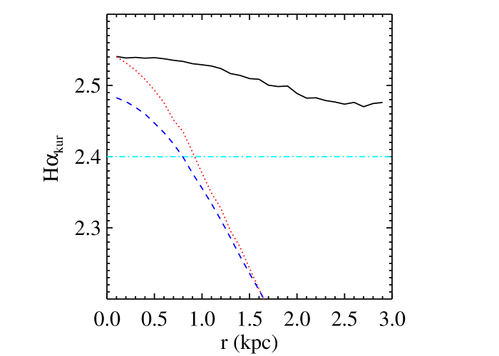
Figure 6: Kurtosis vs. the hole size at fixed circular velocity under a certain assumption of H$\alpha$ light profile distribution. The black-solid curve shows an exponential profile which flattens in the center, $r$ is the radius of the central flat area. Red-dotted and blue-dashed curves represent an exponential and a flat profile with an inner hole, respectively. In these two cases, $r$ is the radius of the hole. The cyan horizontal line marks our boxy source selection criterion ${\rm H}\alpha_{\rm kur}=2.4$.

In the model discussed above, we did not sample the flat part of the rotation curve. We keep in mind that we can get a boxy H$\alpha$ profile when fiber aperture samples out to the flat part of the rotation curve since a lot of H$\alpha$ comes out at a single velocity. Figure 1 of Catinella et al. (2006) shows that the radius where the turn over of rotation curve happens is around $r_{d}$ for the two brightest bins, and for the other less luminous bins, this radius is larger than $r_{d}$, where $r_{d}$ is the exponential disk scale length. However, more than 80% galaxies with boxy H$\alpha$ profiles studied in this work have $r_{d}$ larger than the fiber radius, indicating that we are not going to see very much gas that is on the flat part of the rotation curve. On the other hand, we further check the fraction of galaxies with boxy H$\alpha$ profiles in bins of stellar mass with each mass bin split into three bins of redshift. There is no evidence that the more distant galaxies have higher frequency of boxy H$\alpha$ profiles, suggesting that the larger physical size of the fiber was not playing a role in the frequency of boxy H$\alpha$ profiles. In summary, targeting the flatten part of the rotation curve could not be the dominate reason for the boxy H$\alpha$ profiles.

4.3.2 Dust Obscuration

An interesting question is whether these H$\alpha$ deficit regions are due to a central deficit of star formation or whether they could be due to the effects of dust obscuration. Based on a sample of 10,095 galaxies with bulge$-$disc decompositions in the Millennium Galaxy Catalogue, Driver et al. (2007) infer a large amount of dust in the inner parts of galaxies. They conclude that 71% of all $B-$band photons produced in bulges in the nearby Universe are absorbed by dust. To test the extinction hypothesis for our H$\alpha$ holes, we selected galaxies with boxy H$\alpha$ profiles (${\rm H}\alpha_{\rm kur}<2.4$) and high inclination and stellar mass ($i>60\,^{\circ}$, log $M_{*}/M_{\odot}>$10.8). The projected disk rotation velocities of the galaxies in this sample are larger than the SDSS instrumental resolution, enabling us to measure dust attenuation as a function of velocity. The spectra of the galaxies were normalized to the median flux between 5450 and 5500 Å  where the spectrum is free of strong absorption and emission lines, averaged in the restframe to increase the S/N, and fit with a stellar population synthesis model (see §2.1 for more details). We then examined the continuum-subtracted H$\alpha$ and H$\beta$ line profiles as a function of velocity. Dust attenuation, traced by the H$\alpha$$/$H$\beta$ ratio, is observed to vary with velocity, but only weakly. The mean attenuation correction changes by only 0.1 mag from the disk center ($v=0$ km s^-1) to the outer regions ($v>150$ km s^-1). While our limited velocity resolution is clearly an issue, this change is still much smaller than the amount of attenuation needed to cause the central H$\alpha$ deficit.

5 Summary

We study the structure of H$\alpha$ emission lines in a disk star forming galaxy sample drawn from the SDSS DR7, deriving information on star formation from the H$\alpha$ emission lines by comparing the observed line structures and the simulated line profiles. A large fraction of boxy sources, which is identified by their kurtosis using the criterion ${\rm H}\alpha_{\rm kur}<2.4$, is found from this sample, and this fraction increases with galaxy inclination and flattens at $i=60\,^{\circ}$. Although this trend can be understood in both bi-polar outflow and rotating disk models, three lines of evidence strongly support a disk origin: (1) the boxy source fraction depends more strongly on stellar mass than $\Sigma_{\rm SFR}$; (2) the velocity difference between the two emission components scales strongly with stellar mass with a slope very similar to the classic Tully-Fisher relation; (3) on average the line profiles are very symmetric.

In the rotating disk scenario, a ring-like H$\alpha$ surface brightness distribution, namely, a kpc-scale central H$\alpha$ emission deficient area, is required to produce the boxy line profile. The high fraction $\sim 50$% of boxy sources in high mass galaxies indicates that the H$\alpha$ hole is a common feature. We can not comment on whether this behaviour extends to lower luminosity galaxies because we are limited by the SDSS spectral resolution. The MaNGA survey (Mapping Nearby Galaxies at Apache Point Observatory, Bundy et al. (2015)) plans to obtain integral-field spectroscopy of a representative sample of about 10,000 galaxies above stellar masses of $10^{9}$$M_{\odot}$ with redshift around 0.03. Considering the fairly large fraction of galaxies with boxy H$\alpha$ profiles in massive galaxies, we should expect to see the H$\alpha$ holes in a substantial fraction of MaNGA galaxies. And we will have more information to start investigating the formation mechanism of the H$\alpha$ holes, e.g., star formation suppression associated, with bars, bulges, radio AGN feedback, etc.

References

- Abazajian et al. (2004) Abazajian K., Adelman-McCarthy J. K., Agüeros M. A., Allam S. S., Anderson K., Anderson S. F., Annis J., Bahcall N. A., 2004, AJ, 128, 502
- Abazajian et al. (2009) Abazajian K. N., Adelman-McCarthy J. K., Agüeros M. A., Allam S. S., Allende Prieto C., An D., Anderson K. S. J., Anderson S. F., 2009, ApJS, 182, 543
- Bauer et al. (2005) Bauer A. E., Drory N., Hill G. J., Feulner G., 2005, ApJ, 621, L89
- Bell & de Jong (2001) Bell E. F., de Jong R. S., 2001, ApJ, 550, 212
- Brinchmann et al. (2004) Brinchmann J., Charlot S., White S. D. M., Tremonti C., Kauffmann G., Heckman T., Brinkmann J., 2004, MNRAS, 351, 1151
- Bundy et al. (2015) Bundy K., Bershady M. A., Law D. R., Yan R., Drory N., MacDonald N., Wake D. A., Cherinka B. et al., 2015, ApJ, 798, 7
- Catinella et al. (2006) Catinella B., Giovanelli R., Haynes M. P., 2006, ApJ, 640, 751
- Chen et al. (2010) Chen Y., Tremonti C. A., Heckman T. M., Kauffmann G., Weiner B. J., Brinchmann J., Wang J., 2010, AJ, 140, 445
- Chen et al. (2009) Chen Y., Wild V., Kauffmann G., Blaizot J., Davis M., Noeske K., Wang J., Willmer C., 2009, MNRAS, 393, 406
- Comte & Duquennoy (1982) Comte G., Duquennoy A., 1982, A&A, 114, 7
- de Vaucouleurs (1948) de Vaucouleurs G., 1948, Annales d’Astrophysique, 11, 247
- Driver et al. (2007) Driver S. P., Popescu C. C., Tuffs R. J., Liske J., Graham A. W., Allen P. D., de Propris R., 2007, MNRAS, 379, 1022
- Feulner et al. (2005) Feulner G., Gabasch A., Salvato M., Drory N., Hopp U., Bender R., 2005, ApJ, 633, L9
- Ge et al. (2012) Ge J.-Q., Hu C., Wang J.-M., Bai J.-M., Zhang S., 2012, ApJS, 201, 31
- Greve et al. (2000) Greve A., Neininger N., Tarchi A., Sievers A., 2000, A&A, 364, 409
- Hakobyan et al. (2014) Hakobyan A. A., Nazaryan T. A., Adibekyan V. Z., Petrosian A. R., Aramyan L. S., Kunth D., Mamon G. A., de Lapparent V. et al., 2014, MNRAS, 444, 2428
- Heavens et al. (2004) Heavens A., Panter B., Jimenez R., Dunlop J., 2004, Nature, 428, 625
- Heckman et al. (1990) Heckman T. M., Armus L., Miley G. K., 1990, ApJS, 74, 833
- Hopkins et al. (2006) Hopkins P. F., Hernquist L., Cox T. J., Robertson B., Springel V., 2006, ApJS, 163, 50
- James et al. (2009) James P. A., Bretherton C. F., Knapen J. H., 2009, A&A, 501, 207
- Kauffmann et al. (2003) Kauffmann G., Heckman T. M., Tremonti C., Brinchmann J., Charlot S., White S. D. M., Ridgway S. E., Brinkmann J., 2003, MNRAS, 346, 1055
- Kennicutt (1998) Kennicutt Jr. R. C., 1998, ARA&A, 36, 189
- Kroupa (2001) Kroupa P., 2001, MNRAS, 322, 231
- Lehnert & Heckman (1996) Lehnert M. D., Heckman T. M., 1996, ApJ, 462, 651
- Lehnert et al. (1999) Lehnert M. D., Heckman T. M., Weaver K. A., 1999, ApJ, 523, 575
- Lupton et al. (2001) Lupton R., Gunn J. E., Ivezić Z., Knapp G. R., Kent S., 2001, in F. R. Harnden Jr., F. A. Primini, & H. E. Payne ed., Astronomical Data Analysis Software and Systems X Vol. 238 of Astronomical Society of the Pacific Conference Series, The SDSS Imaging Pipelines. pp 269–+
- Nair & Abraham (2010) Nair P. B., Abraham R. G., 2010, ApJ, 714, L260
- Noeske et al. (2007) Noeske K. G., Weiner B. J., Faber S. M., Papovich C., Koo D. C., Somerville R. S., Bundy K., Conselice C. J., 2007, ApJ, 660, L43
- Padilla & Strauss (2008) Padilla N. D., Strauss M. A., 2008, MNRAS, 388, 1321
- Pérez-González et al. (2003) Pérez-González P. G., Zamorano J., Gallego J., Aragón-Salamanca A., Gil de Paz A., 2003, ApJ, 591, 827
- Ryder & Dopita (1994) Ryder S. D., Dopita M. A., 1994, ApJ, 430, 142
- Salim et al. (2007) Salim S., Rich R. M., Charlot S., Brinchmann J., Johnson B. D., Schiminovich D., Seibert M., Mallery R., 2007, ApJS, 173, 267
- Schlegel et al. (1998) Schlegel D. J., Finkbeiner D. P., Davis M., 1998, ApJ, 500, 525
- Strauss et al. (2002) Strauss M. A., Weinberg D. H., Lupton R. H., Narayanan V. K., Annis J., Bernardi M., Blanton M., Burles S., 2002, AJ, 124, 1810
- Thomas et al. (2005) Thomas D., Maraston C., Bender R., Mendes de Oliveira C., 2005, ApJ, 621, 673
- Tremonti et al. (2004) Tremonti C. A., Heckman T. M., Kauffmann G., Brinchmann J., Charlot S., White S. D. M., Seibert M., Peng E. W., et al., 2004, ApJ, 613, 898
- Tully & Fisher (1977) Tully R. B., Fisher J. R., 1977, A&A, 54, 661
- Westmoquette et al. (2009) Westmoquette M. S., Smith L. J., Gallagher J. S., Trancho G., Bastian N., Konstantopoulos I. S., 2009, ApJ, 696, 192
- York et al. (2000) York D. G., Adelman J., Anderson Jr. J. E., Anderson S. F., Annis J., Bahcall N. A., Bakken J. A., Barkhouser R., 2000, AJ, 120, 1579
- Zheng et al. (2007) Zheng X. Z., Bell E. F., Papovich C., Wolf C., Meisenheimer K., Rix H., Rieke G. H., Somerville R., 2007, ApJ, 661, L41