Multi-Source Multi-View Clustering via Discrepancy Penalty

Abstract

With the advance of technology, entities can be observed in multiple views. Multiple views containing different types of features can be used for clustering. Although multi-view clustering has been successfully applied in many applications, the previous methods usually assume the complete instance mapping between different views. In many real-world applications, information can be gathered from multiple sources, while each source can contain multiple views, which are more cohesive for learning. The views under the same source are usually fully mapped, but they can be very heterogeneous. Moreover, the mappings between different sources are usually incomplete and partially observed, which makes it more difficult to integrate all the views across different sources. In this paper, we propose MMC (Multi-source Multi-view Clustering), which is a framework based on collective spectral clustering with a discrepancy penalty across sources, to tackle these challenges. MMC has several advantages compared with other existing methods. First, MMC can deal with incomplete mapping between sources. Second, it considers the disagreements between sources while treating views in the same source as a cohesive set. Third, MMC also tries to infer the instance similarities across sources to enhance the clustering performance. Extensive experiments conducted on real-world data demonstrate the effectiveness of the proposed approach.

I Introduction

With the advance of technology, most of entities can be observed in multiple views. Multiple views containing different types of features can be used for clustering. Multiple view clustering [1, 2, 3] aims to enhance clustering performance by integrating different views. Moreover, as the information explodes, we can get information from multiple sources. Each source can contain multiple views that are fully aligned and available for clustering. Combining data from multiple sources, multiple views may help us get better clustering performance.

However, several difficulties prevent us from combining different sources and views. First, the views may be very heterogeneous. Different views may have different feature spaces and distributions. Second, the instances mapping between different sources may be incomplete and partially observed. Different sources may have different instance sets, which means the instance mapping between different sources is not fully mapped. Also in real-world problems, the instance mapping is often partially observed. We may only get part of the instance mapping between different sources. Third, the views in one source are generally more cohesive than the views across different sources. This is very different from the traditional multi-view clustering problem.

A good example is the social networks shown in Fig. 1. People usually use several social network services simultaneously, e.g., those provided by Twitter and Foursquare. Each social network is an independent source containing several views that describe different aspects of the social network. We can use the profile information of users for both Twitter and Foursquare (view 3 in Fig. 1), the social connections of users (view 2 in Fig. 1), location check-in history, etc. Views in a single source describe the characters of the same set of users and focus on different aspects. The views in Twitter focus on the social activity aspects, while the views in Foursquare focus more on the location based aspects. Since not all people use both Twitter and Foursquare, the user mapping between Twitter and Foursquare is incomplete and not one-to-one. Furthermore, not all the shared users link their Twitter accounts with their Foursquare accounts. We can only observe part of the mapping between Twitter and Foursquare.

Multi-view clustering [1, 4, 5] aims to utilize the multiple representations of instances in different features spaces to get better clustering performance. However, most of the previous methods are based on the assumption that all the views are fully mapped/aligned. They cannot deal with the multi-source multi-view scenario with incomplete/partial mapping across sources. Although there are some previous studies on dealing with multiple incomplete view clustering [6, 7, 8, 9], none of them are suitable for multi-source multi-view scenario. They either cannot extend to more than two views or they do not treat the views in one source as a cohesive set. All of the previous methods only use the known mapping information. Furthermore, none of them try to extend the known mapping information to help improve clustering.

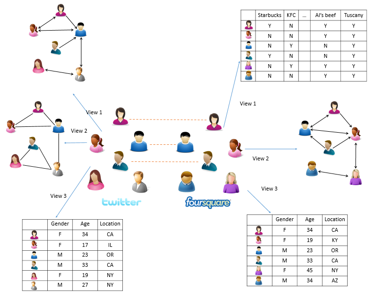
Figure 1: An Example of Social Networks. Twitter and Foursquare are two sources. Twitter contains user connection view, user interaction view and user profile view, while Foursquare contains user connection view, user check-in location view, user profile view. The user mapping between Twitter and Foursquare is incomplete and partially observed.

These challenges and emerging applications call for novel clustering methods which can deal with multiple sources multiple views situations. In this paper, we propose MMC (Multi-source Multi-view Clustering) to integrate multiple sources for better clustering results. The main contributions of this paper are summarized as follows:

1. This paper is the first one to investigate the multi-source multi-view clustering problem, where multiple sources containing multiple views are available for clustering and the instance mappings between sources are incomplete and partially known.

2. We develop a method MMC, based on collective spectral clustering with discrepancy penalty within and between sources. MMC appreciates the cohesiveness of all the views in each source by pushing the latent feature matrice of the views in one source to a consensus for each source. MMC also considers the cross-source discrepancy by minimize the difference among the consensus latent feature matrices of different sources.

3. The proposed MMC not only generates clusters from multiple sources but also tries to infer the unknown instance similarity mapping between sources to improve the clustering performance. By using the learned consensus latent feature matrices of different sources and the incomplete/partial mappings across sources, MMC generates the instance similarities across different sources, which will in turn help enhance the clustering performance.

4. The proposed MMC is not limited to the multiple sources multiple views problem. In real-world applications, we may have multiple partial aligned views, i.e., views with different numbers of instances. We can group the views into groups where each group has the same set of instances. Thus each group can be viewed as a source and our method can be applied.

The experiment results on three groups of real data show the effectiveness of the proposed method by comparing it with other state-of-art methods.

II Problem Formulation

In this section, we will first define the problem of multi-source multi-view clustering. Then we will start from the single source problem to develop the objective function for multi-source multi-view clustering problem.

II-A Problem Definition

Before we define the problem of multi-source multi-view clustering, we summarize the notations in Table I. Let $\mathcal{S}=\{S^{k}\}_{k=1}^{K}$ denote the set of the $K$ available sources. For each $S^{k}$, we have $S^{k}=\{X_{i}^{k}\}_{i=1}^{v_{k}}$, where $X_{i}^{k}$ denotes the $i$-th view in source $k$ and $v_{k}$ denotes the number of views in source $k$. We assume that source k $(1\leq k\leq K)$ contains $n_{k}$ instances. Let $\mathcal{M}=\{M^{(i,j)}\}_{1\leq i,j\leq K}$ be the known instance mappings between sources, where $M^{(i,j)}\in\mathbb{R}_{+}^{n_{i}\times n_{j}}$ denotes the instance mapping between sources i and j, and its element is defined by

$$M_{a,b}^{(i,j)}=\begin{cases}1&\text{instance $a$ in source $i$ is mapped to }\\ &\text{instance $b$ in source $j$}.\\ 0&\text{otherwise.}\end{cases}$$ (1)

TABLE I: Summary of symbols and their meanings

Symbols Description K Number of sources. $v_{k}$ Number of views for source $k$. $n_{k}$ Number of instances in source $k$. $c_{k}$ Number of clusters for source $k$. $X^{k}_{i}$ i-th view in source $k$ $K^{k}_{i}$ Kernel matrix for the $i$-th view in source $k$ $K_{U}$ Kernel matrix of the matrix $U$ $L^{k}_{i}=(D^{k}_{i})^{-1/2}K^{k}_{i}(D^{k}_{i})^{-1/2}$ Normalized graph Laplacian for the i-th view in source $k$, where $D^{k}_{i}$ is a diagonal matrix consisting of the row sums of $K_{i}^{k}$. $M^{(i,j)}\in\mathbb{R}^{n_{i}\times n_{j}}$ Instance mapping between source $i$ and $j$. $W^{(i,j)}\in\mathbb{R}^{n_{i}\times n_{j}}$ Indicator matrix between source $i$ and $j$ $\alpha^{k}_{i}$ Importance of view $i$ in source $k$ $\beta^{(i,j)}$ Importance of penalty between source $i$ and $j$ $U^{k}_{i}\in\mathbb{R}^{n_{k}\times c_{k}}$ Latent feature matrix for view $i$ in source $k$ $U^{k*}\in\mathbb{R}^{n_{k}\times c_{k}}$ Consensus latent feature matrix for source $k$

Our goal is to cluster the instances into $c_{k}$ clusters for each source k, while considering the other sources by using the cross-source mapping in $\mathcal{M}$.

II-B Single Source Multiple Views Clustering

Clustering with multiple views within a single source can be seen as traditional multi-view clustering problem. However, in order to incorporate the cross-source disagreement, we would like to get a consensus clustering solution for each source. Let $K^{k}_{i}$ be the positive semi-definite similarity matrix or kernel matrix for view $i$ in source $k$. The corresponding normalized graph Laplacian will be $L^{k}_{i}={D^{k}_{i}}^{-1/2}K^{k}_{i}{D^{k}_{i}}^{-1/2}$, where $D^{k}_{i}$ is a diagonal matrix with the diagonal elements be the row sums of $K^{k}_{i}$. To perform spectral clustering for a single view $i$ in source $k$, as shown in [3, 10, 11], we only need to solve the following optimization problem for the normalized graph Laplacian $L^{k}_{i}$:

$$\max_{U^{k}_{i}\in\mathbb{R}^{n_{k}\times c_{k}}}~{}tr((U^{k}_{i})^{T}L^{k}_{i}U^{k}_{i}),~{}~{}s.t.(U^{k}_{i})^{T}U^{k}_{i}=\mathit{I},$$ (2)

where $tr$ denotes the matrix trace, and $U^{k}_{i}$ can be seen as a latent feature matrix of view $i$ in source $k$, which can be given to the k-means algorithm to obtain cluster memberships. For clustering multiple views in the same source, we have to consider the disagreement between different views. We enforce the learned latent feature matrix for each view to look similar by regularizing them towards a common consensus.

Similar to the regularization in [3], we define the discrepancy/dissimilarity between two latent feature matrices as:

$$D(U^{k}_{i},U^{k}_{j})=\|K_{U^{k}_{i}}-K_{U^{k}_{j}}\|_{F}^{2},$$ (3)

where $K_{U^{k}_{i}}$ and $K_{U^{k}_{j}}$ are the similarity/kernel matrices for $U^{k}_{i}$ and $U^{k}_{j}$, and $\|.\|_{F}$ denotes the Frobenius norm of the matrix. We use linear kernel as the similarity measure in Eq. (3). Thus, we get $K_{U^{k}_{i}}=U^{k}_{i}(U^{k}_{i})^{T}$ and $K_{U^{k}_{j}}=U^{k}_{j}(U^{k}_{j})^{T}$. Using the properties of trace and the fact that $(U^{k}_{i})^{T}U^{k}_{i}=\mathit{I}$, $(U^{k}_{j})^{T}U^{k}_{j}=\mathit{I}$, Eq. (3) can be rewritten as follows:

$$\begin{split}&D(U^{k}_{i},U^{k}_{j})=\|U^{k}_{i}(U^{k}_{i})^{T}-U^{k}_{j}(U^{k}_{j})^{T}\|_{F}^{2}\\ &=tr\left(U^{k}_{i}(U^{k}_{i})^{T}+U^{k}_{j}(U^{k}_{j})^{T}-2U^{k}_{i}(U^{k}_{i})^{T}U^{k}_{j}(U^{k}_{j})^{T}\right)\\ &=2c_{k}-2tr(U^{k}_{i}(U^{k}_{i})^{T}U^{k}_{j}(U^{k}_{j})^{T}).\end{split}$$ (4)

Ignoring the constant terms, we can get the discrepancy between two different latent feature matrices:

$$D(U^{k}_{i},U^{k}_{j})=-tr(U^{k}_{i}(U^{k}_{i})^{T}U^{k}_{j}(U^{k}_{j})^{T}).$$ (5)

Then $D(U^{k}_{i},U^{k*})=-tr(U^{k}_{i}(U^{k}_{i})^{T}U^{k*}(U^{k*})^{T})$ is the discrepancy between the $i$-th view and the consensus. Considering the discrepancy/dissimilarity between each view and the consensus in the same source, the objective function for clustering all the views within the $k$-th source will be as follows:

$$\begin{split}\max_{\{U^{k}_{i}\},{U^{k*}}}\mathcal{J}_{k}&=\sum_{i=1}^{v_{k}}\left(tr({U^{k}_{i}}^{T}L^{k}_{i}U^{k}_{i})+\alpha^{k}_{i}tr(U^{k}_{i}{U^{k}_{i}}^{T}U^{k*}{U^{k*}}^{T})\right),\\ &\textit{s.t.}~{}~{}{U^{k}_{i}}^{T}U^{k}_{i}=\mathit{I},\forall 1\leq i\leq v_{k},{U^{k*}}^{T}U^{k*}=\mathit{I}\end{split}$$ (6)

where $\mathcal{J}_{k}$ is the objective function for source $k$, $U^{k}_{i}$ is the latent feature matrix for the $i$-th view in source $k$, $U^{k*}$ is the consensus latent feature matrix for source $k$, and $\alpha^{k}_{i}$ is the relative importance of view $i$ in source $k$.

II-C Multiple Sources Multiple Views Clustering

In this section, we will derive the objective function for Multi-source Multi-view Clustering problem. We model it as a joint matrix optimization problem.

In order to incorporate multiple sources, we need to add penalty between sources to the single source multiple views clustering objective function. To appreciate the cohesiveness of the views within one source, we learn the consensus latent feature matrix for each source and only penalize the discrepancy between those consensus latent feature matrices.

Similar to the discrepancy function across views within one source, the penalty function across sources should consider the discrepancy between the consensus clustering results for the sources. Since the mappings between sources are incomplete and partially known, we cannot directly apply the same penalty function as in the single source multiple views clustering objective function. However, by using the mapping matrices, we can project the learned latent feature matrix from one source to other sources, ${M^{(i,j)}}^{T}U^{i*}$ can be seen as projection of the instance in source $i$ to the instances in source $j$. The penalty function for discrepancy between source $i$ and source $j$ is as follow:

$$\widetilde{D}(U^{i*},U^{j*})=\|{M^{(i,j)}}^{T}U^{i*}({M^{(i,j)}}^{T}U^{i*})^{T}-U^{j*}{U^{j*}}^{T}\|_{F}^{2}.$$ (7)

Observing that the known mapping between two sources is one-to-one and it is reasonable to assume that the unknown part is one-to-at-most-one, which means one instance in one source can be mapped to at most one instance in the other source. So we can approximately assume that $M^{(i,j)}M^{(i,j)T}=I$ to help simplify the penalty function. The Eq. 7 can be expressed as:

$$tr\left(\left({M^{(i,j)}}^{T}U^{i*}U^{i*T}M^{(i,j)}-U^{j*}U^{j*T}\right)\left({M^{(i,j)}}^{T}U^{i*}U^{i*T}M^{(i,j)}-U^{j*}U^{j*T}\right)\right)$$ (8)

Using the fact that $U^{i*T}U^{i*}=I$, $tr(U^{i*T}U^{i*})=c_{i}$, and $M^{(i,j)}M^{(i,j)T}=I$, and ignoring the constant terms, the penalty function for discrepancy is

$$\small\widetilde{D}(U^{i*},U^{j*})=-tr\left(U^{j*}U^{j*T}{M^{(i,j)}}^{T}U^{i*}U^{i*T}M^{(i,j)}\right)$$ (9)

Adding the penalty function between sources to the single source multiple views clustering objective function for all the sources, we get

$$\begin{split}\max_{U^{k}_{i},U^{k*}(1\leq k\leq K,1\leq i\leq v_{k})}\mathcal{O}=\sum_{k=1}^{K}\mathcal{J}_{k}-\sum_{i\neq j,1\leq i,j\leq K}\beta^{(i,j)}\widetilde{D}(U^{i*},U^{j*}),\end{split}$$

where $\beta^{(i,j)}\geq 0$ is a parameter controlling the balance between the objective function for individual source and the inconsistency across sources.

III Optimization and MMC framework

The proposed MMC framework simultaneously optimizes the latent featue matrices in multiple sources and infers the cross-source instance similarity mappings to help enhance the clustering performance. To optimize the objective function in Eq. (II-C), we employ an alternating scheme, that is, we optimize the objective function with respect to one variable while fixing others. Basically, we optimize the objective function using two stages. First, maximizing $\mathcal{O}$ over $U^{k}_{i}$s with fixed $U^{k*}$s. Second, maximizing $\mathcal{O}$ over $U^{k*}$s with fixed $U^{k}_{i}$s. We repeat these two steps, until it converges.

Solving the optimization, we can iteratively learn the latent feature matrices for each source. However, when only a small portion of instances mapping between sources are observed, the clustering performance is affected by the incompleteness of the instance mapping across sources. Inferring the exact instance mapping is really challenging and usually additional information is required to infer such anchor link [12, 13]. However, instead of inferring the exact instance mapping, we can try to infer the similarity mapping. This idea is based on the Principle of Transitivity on Similarity:

Theorem III.1.

Instances similar to the same instance in different sources should be similar.

Fig. 2 illustrates the principle.

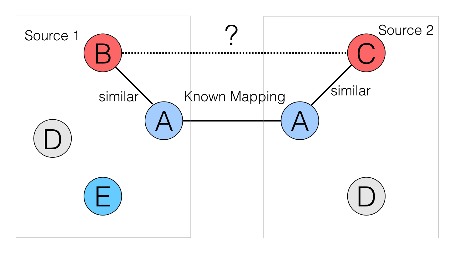
Figure 2: Principle of Transitivity on Similarity.

In Fig. 2, B and C are both similar to A in different sources. Given the known mapping between A in the two sources, we can infer that B and C are similar. MMC tries to use the similarity transitivity principle to help infer the cross-source instance similarity and to help improve the clustering performance. Next, we will talk about each step in the MMC framework in detail.

III-A Initialization

Since the efficiency of the iterative optimization is affected by the initialization step, in this paper, we learn the initial value of $U_{i}^{k}$ and $U^{k*}$ rather than random initialization. For each $U_{i}^{k}$, we solve Eq. (2) to get an initial value. As we described in the previous section, Eq. (2) is just the objective function for single view clustering, without considering the relation among views and sources. The solution $U^{k}_{i}$ is given by the top-$c_{k}$ eigenvectors of the Laplacian $L_{i}^{k}$.

For each $U^{k*}$, we just solve Eq. (6) to get the initialization value with the initial $U^{k}_{i}$. The objective function can be written as:

$$\small\centering\begin{split}\max_{U^{k*}}~{}&tr\left({U^{k*}}^{T}\left(\sum_{i=1}^{v_{k}}\alpha^{k}_{i}U^{k}_{i}{U^{k}_{i}}^{T}\right)U^{k*}\right),\\ &\textit{s.t.}~{}~{}{U^{k*}}^{T}U^{k*}=\mathit{I}\end{split}\@add@centering$$ (10)

The solution is given by the top-$c_{k}$ eigenvectors of the modified Laplacian $\sum_{i=1}^{v_{k}}\alpha^{k}_{i}U^{k}_{i}{U^{k}_{i}}^{T}$.

In the previous section, we assume that the mapping matrix between two sources is semi-orthogonal, i.e., $M^{(i,j)}M^{(i,j)T}=I$. However, we can only get part of the mapping information due to the incompleteness and partial known property of real-world problem. The mapping matrix between two sources can be expressed in two parts $M_{0}^{(i,j)}$ and $M_{1}^{i,j}$:

$$M^{(i,j)}=\begin{bmatrix}M_{0}^{(i,j)}&0\\ 0&M_{1}^{(i,j)}\end{bmatrix},$$ (11)

where $M_{0}^{(i,j)}$ represents the known mapping between source $i$ and $j$ and $M_{1}^{(i,j)}$ represents the unknown part.

It is easy to find that $M_{0}^{(i,j)}M_{0}^{(i,j)T}=I$. We only need to initialize the unknown part to make it semi-orthogonal. One natural way to estimate the unknown mapping is to use the instance similarity among the instances between two sources. Using the similarity transitivity principle, the instance similarity between two sources $i$ and $j$ can be estimated by: $\small K_{U^{i*}}\begin{bmatrix}M_{0}^{(i,j)}&0\\ 0&0\end{bmatrix}K_{U^{j*}},$ where $K_{U^{i*}}$ and $K_{U^{j*}}$ are the two kernel matrices for latent feature $U^{i*}$ and $U^{j*}$. It is worth to note that the kernel matrices $K_{U^{i*}}$ and $K_{U^{j*}}$ can be seen as the similarity matrices of the latent features for sources $i$ and $j$. The similarity transitivity principle allows us to use the known instance mapping as a bridge to connects unmapped instances in two sources. Using Fig. 2 as an example, $\left(K_{U^{i*}}\right)_{b,a}$ provides the similarity between instances B and A in source $i$, while $\left(K_{U^{j*}}\right)_{a,c}$ provides the similarity between instances A and C in source $j$. If both instances A in both sources $i$ and $j$ are mapped through $M^{(i,j)}$, $\left(K_{U^{i*}}\begin{bmatrix}M_{0}^{(i,j)}&0\\ 0&0\end{bmatrix}K_{U^{j*}}\right)_{b,c}$, denoted by $(\widetilde{M}^{(i,j)})_{b,c}$, will provide the estimated similarity between instance B in source $i$ and instance C in source $j$. So for the unmapped instances, we can have an estimated similarity mapping $\widetilde{M}_{1}^{(i,j)}$. Then we can orthogonalize it using SVD or other orthogonalization methods.

III-B Maximizing $\mathcal{O}$ over $U^{k}_{i}$s with fixed $U^{k*}$s

With fixed $U^{k*}$s, for each $U^{k}_{i}$ we only need to maximize part of $\mathcal{J}_{k}$.

$$\small\begin{split}\max_{U^{k}_{i}}~{}\mathcal{L}&=tr({U^{k}_{i}}^{T}L^{k}_{i}{U^{k}_{i}})+\alpha^{k}_{i}tr({U^{k}_{i}}{U^{k}_{i}}^{T}U^{k*}{U^{k*}}^{T})\\ &=tr({U^{k}_{i}}^{T}(L^{k}_{i}+\alpha^{k}_{i}U^{k*}{U^{k*}}^{T}){U^{k}_{i}})\\ &\textit{s.t.}~{}~{}{U^{k}_{i}}^{T}U^{k}_{i}=\mathit{I}\end{split}$$ (12)

This is a standard spectral clustering objective on source $k$ view $i$ with modified graph Laplacian $L^{k}_{i}+\alpha^{k}_{i}U^{k*}{U^{k*}}^{T}$. According to [11], the solution $U^{k}_{i}$ is given by the top-$c_{k}$ eigenvectors of this modified Laplacian. With fixed $U^{k*}$s, we can calculate each $U^{k}_{i}$ to maximize the objective function.

III-C Maximizing $\mathcal{O}$ over $U^{k*}$s with fixed $U^{k}_{i}$s

With fixed $U^{k}_{i}$s, for each $U^{k*}$, we only need to maximize:

where

$$L^{k*}=\sum_{i=1}^{v_{k}}\alpha^{k}_{i}U^{k}_{i}{U^{k}_{i}}^{T}+\sum_{j\neq k}\beta^{(k,j)}M^{(k,j)}U^{j*}U^{j*T}{M^{(k,j)}}^{T}$$

The solution $U^{k*}$ is given by the top-$c_{k}$ eigenvectors of this modified Laplacian $L^{k*}$. Thus, with fixed $U^{k}_{i}$s, we can calculate the consensus $U^{k*}$ for each of the sources to maximize the objective function.

III-D Infer the Similarity Mapping between Sources

Using above optimization method, we can iteratively learn the latent feature matrices for each source. However, when the number of partially observed mapping is limited, i.e., when only a small number of instances mapping between sources are observed, the estimated initial similarity mapping between two sources may not be accurate. Hence the improvement of clustering performance is limited.

Based on the similarity transitivity principle, MMC proposes to use the learned latent feature matrices for multiple sources to help infer the similarity mapping across sources.

Similar to the initialization, we use the instance mapping between two sources as a bridge to help transfer the similarity. The new estimated instance similarities between two sources can be written as:

$$\widetilde{M}^{(i,j)}=K_{U^{i*}}M^{(i,j)}K_{U^{j*}},$$ (14)

where $K_{U^{i*}}$ and $K_{U^{j*}}$ are the two kernel matrices for latent feature matrices $U^{i*}$ and $U^{j*}$. In our experiment, we use linear kernel for the latent feature matrices.

This estimated similarity mapping includes every instance across two sources. However, we want to preserve the already known instance mapping and only update the instance similarity mapping for instances whose mappings are unknown. We introduce the indicator matrix $W^{i,j}$, which has the same dimension as $M^{(i,j)}$ and was initialized with only 0 and 1. $W^{(i,j)}_{ab}$ equals to 1 if the mapping between $a$-th instance from source $i$ and the $b$-th instance from source $j$ is known, and 0 if unknown. The similarity mapping between source $i$ and source $j$ and is updated as follows:

$$M^{(i,j)}\leftarrow W^{(i,j)}\circ M^{(i,j)}+(\mathbf{1}-W^{(i,j)})\circ\widetilde{M}^{(i,j)},$$ (15)

where $\circ$ indicates the element-wise multiplication, $\widetilde{M}^{(i,j)}=U^{i*}{U^{i*}}^{T}M^{(i,j)}U^{j*}{U^{j*}}^{T}$ and $\mathbf{1}$ is an all-one matrix. By using the indicator matrix $W^{(i,j)}$ and element-wise multiplication, we can only update the unknown part of the mapping, and preserve the known part. Once we have a better mapping across sources, it will help learn better latent feature matrices. The better latent feature matrices will in-turn help infer the similarity mapping. This iteration continues until it converges.

III-E MMC framework

The algorithm for the MMC framework is shown as Algorithm 1. We first calculate the kernel matrices and the corresponding normalized graph Laplacian matrices for every view. In all the experiments throughout the paper, we use Gaussian kernel for computing the similarities unless mentioned otherwise. The standard deviation of the kernel is set equal to the median of the pair-wise Euclidean distances between the data points. We then initialize the latent feature matrices $\{U_{i}^{k}\}$, $\{U^{k*}\}$ and the instance mappings $M^{(i,j)}$. Then we iteratively update $U_{i}^{k}$s, $U^{k*}$s and $M^{(i,j)}$s until they all converge.

Algorithm 1 MMC framework

0:  Data matrices for every view from each source $\{X^{k}_{i}\}$. Instance mappings between sources $\{M^{(i,j)}\}$. Indicator matrices $\{W^{(i,j)}\}$. The number of clusters for each source $\{c_{k}\}$. Parameters $\{\alpha^{k}_{i}\}$ and $\{\beta^{(i,j)}\}$.

0:  Clustering results for each source.

1:  Calculate $K^{k}_{i}$ and $L^{k}_{i}$ for every $k$ and $i$.

2:  Initialize $U_{i}^{k}$ for every $k$ and $i$.

3:  Initialize $U^{k*}$ by solving Eq.(10).

4:  repeat

5:     repeat

6:        Update each $U_{i}^{k}$ by solving Eq. (12).

7:        Update each $U^{k*}$ by solving Eq. (13).

8:     until objective function $\mathcal{O}$ converges.

9:     Update the similarity mappings using Eq. (15).

10:  until mappings between sources converge.

11:  Apply k-means on $U^{k*}$ for every source $k$.

IV Experiments and Results

In this section, we compare MMC framework with a number of baselines on three real-world data sets.

IV-A Comparison Methods

We compare the proposed MMC method with several state-of-art methods. Since no previous methods can be directly applied to the multi-source multi-view situation, in order to compare with the previous methods, we make some changes. The details of comparison methods is as follows:

• MMC: MMC is the clustering framework proposed in this paper, which applies collective spectral clustering with discrepancy penalty across sources. The parameter $\alpha$ is set to 0.1 and $\beta$ is set to 1 for all the views and sources throughout the experiment.

• Concat: Feature concatenation is one way to integrate all the views. We concatenate views within each source, so each source is a concatenated view. Since the instances between sources are not fully aligned, we extend each source by adding pseudo instances (average features). Thus, sources are fully aligned after extension. We then apply PCA and k-means to get the clustering results.

• Sym-NMF Symmetric non-negative matrix factorization is proposed in [14] as a general framework for clustering. It factorizes a symmetric matrix containing pairwise similarity values. To apply Sym-NMF to multi-source multi-view situation, we apply Sym-NMF to every view from each source to get the latent feature matrices. Then we combine all the latent feature matrices in the same source to produce the final clustering results.

• MultiNMF: MultiNMF is one of the state-of-art multi-view clustering methods based on joint nonnegative matrix factorization [15]. MultiNMF formulates a joint matrix factorization process with the constraint that pushes clustering solution of each view towards a common consensus instead of fixing it directly. Throughout the experiment, the parameter $\lambda_{v}$ is set to 0.01 as in the original paper.

• CoReg: CoReg is the centroid based multi-view clustering method proposed in [3]. It aims to get clusters that are consistent across views by co-regularizing the clustering hypotheses. Throughout the experiment, the parameter $\lambda_{v}$ is set to 0.01 as suggested in the original paper.

• CGC: CGC [8] is the most recent work that deals with many-to-many instance relationship, which is similar to incomplete instance mapping. In order to run the CGC algorithm, we generated the relations between views within one source, which is complete one-to-one mapping. We also generate the relations between views across sources, which is incomplete and partially known. We run CGC on all the views across sources and report the best performance for each source. In the experiment, the parameter $\lambda$ is set to 1 as suggested in the original paper.

It is worth to note that the two multi-view clustering methods MultiNMF and Co-Reg only work with views that are fully aligned. In our experiments, only views from the same source are fully mapped/aligned. Views across different sources are partially mapped. We apply MultiNMF and Co-Reg in two ways.

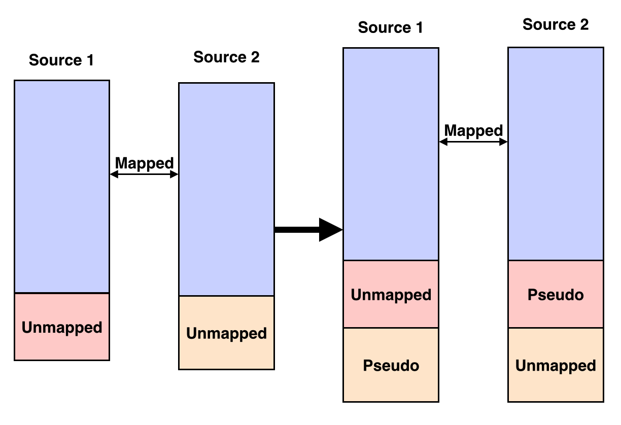
Figure 3: Source alignment

The first way is to apply them to every single source, denoted as MultiNMF-S and CoReg-S. Thus, both MultiNMF-S and Co-Reg-S only co-regularize the views within a source without considering the discrepancy between sources. The second way is to apply MultiNMF and Co-Reg to multiple sources, denoted as MultiNMF-M and CoReg-M. However, the views across sources are not fully mapped/aligned. In order to apply MultiNMF and Co-Reg, we align the sources by adding average pseudo instances to every source. As shown in Fig. 3, for the unmapped instances in one source, we created the corresponding pseudo instances in other sources. Thus, the instances from different sources are fully mapped. MultiNMF and Co-Reg are then applied to all the aligned views, and performance is reported for every source.

In our experiments, we use Gaussian kernel for computing the similarities unless mentioned otherwise. The standard deviation of the kernel is set equal to the median of the pair-wise Euclidean distances between the data points. K-means is used to get clustering results for all the methods. For each setting, we run k-means 20 times and report the average performance.

IV-B Dataset

In this paper, three groups of real-world data sets are used to evaluate the proposed MMC method. The important statistics of them are summarized in Table II.

TABLE II: Statistics of the datasets

data size # view # cluster Dutch 2000 6 10 USPS 2000 2 10 English 1200 2 6 Translation 1200 2 6 BBC 352 2 6 Reuters 294 2 6 Guardian 302 2 6

• Dutch-USPS This data set comes from two sources, UCI Handwritten Dutch digit numbers and USPS digit data. The first source, Dutch, consists of 2000 examples of handwritten numbers ’0’-’9’ (200 examples per class) extracted from a collection of Dutch utility maps. All the examples have been digitized in binary images. Each example is represented in the following six views: (1) 76 Fourier coefficients of the character shapes, (2) 216 profile correlations, (3) 64 Karhunen-Love coefficients, (4) 240 pixel averages in $2\times 3$ windows, (5) 47 Zernike moments, and (6) 6 morphological features. The second source, USPS, consists of digit images with size $16\times 16$ for numbers ‘0’-‘9’. We randomly select 2000 examples corresponding to the examples in first source. From USPS data, we extract two views, the original pixel feature with dimension of 256 and the Gaussian similarity matrix between examples with dimension of 2000.

• English-Translations: This data contains two sources, the original Reuters news documents written in English, and the machine translations in other four languages (French, German, Spanish and Italian) in 6 topics [16]. From the first source, English, we use the document-term matrix and the cosine similarity matrix of the documents as two views. From the second source, Translation, we extract the document-term matrices from French and German as two views. We randomly sample 1200 documents from the first source in a balanced manner, with each category having 200 documents. We then select the corresponding 1200 documents from the second source.

• News Text data: This news data has three sources: BBC, Reuters, and The Guardian. In total there are 948 news articles covering 416 distinct news stories from the period February to April 2009. Thus, the articles from these three sources are naturally partially mapped. Of these distinct stories, 169 were reported in all three sources, 194 in two sources, and 53 appeared in a single news source. Each story was annotated with one of the six topical labels: business, entertainment, health, politics, sport, technology. From each source, we extract two views, the document-term matrix and the cosine similarity matrix. From the three sources, we create three sets of data, BBC-Reuters (239 mapped instances), BBC-Guardian (250 mapped instances) and Reuters-Guadian (212 mapped instances).

It is worth noting that both Dutch-USPS and English-Translation data are one-to-one fully mapped. In our experiments, we randomly delete part of the mappings across different sources.

IV-C Results

The results for Dutch-USPS data and English-Translation data are shown in Table III. The results are obtained under 60% known mappings . We report the NMI (Normalized Mutual Information) for each source in Table III.

From Table III, we can observe that the proposed MMC framework outperforms all the other comparison methods on both Dutch-USPS and English-Translation data. For the Dutch-USPS data, although CoReg-M and CGC are close to MMC (less than 4%) on Dutch, MMC outperforms the other methods on USPS by at least 10 %. We can also observe that MultiNMF-M and CoReg-M perform better than MultiNMF-S and CoReg-S on Dutch-USPS. However, the performance of the multi-source methods is worse than single-source method on English-Translation. This suggests that combining multiple sources only using the incomplete instance mappings may even hurt the performance. The proposed MMC methods, however, iteratively discovers the similarity among unmapped instances and uses the similarity to help learning.

We also reported the results on three sets of the news text data (BBC-Reuters, BBC-Guardian and Reuters-Guardian) in Table IV. From Table IV, we can see that MMC outperforms other comparison methods by a large margin in most cases. On Reuters-Guardian, although MultiNMF-M is slightly better than MMC on Guardian, MMC is still better than all the other baselines on Reuters.

From Table III and Table IV, we can observe that MMC outperforms other comparison methods in most cases for all the three groups of data. We can also conclude that MMC reduces the impact of negative transfer by iteratively learns the similarity among unmapped instances and takes advantage of it. The other reason why MMC can have a better performance for all the sources is that MMC treats the views within each source as a cohesive unit for clustering while considering discrepancy/disagreements between sources.

TABLE III: NMI for Dutch-USPS and English-Translation at 60% cross source mapping known

Method Dutch USPS English Translation Concat 0.5734 0.3916 0.1914 0.1621 Sym-NMF 0.7778 0.3005 0.2783 0.1527 MultiNMF-S 0.5382 0.4010 0.3413 0.2708 MultiNMF-M 0.7585 0.4700 0.342 0.2164 CoReg-S 0.7503 0.4044 0.3381 0.2874 CoReg-M 0.7886 0.5257 0.2187 0.2198 CGC 0.7851 0.2780 0.2636 0.2536 MMC 0.8248 0.6348 0.3528 0.3073

TABLE IV: NMI for News Text Data

Method BBC-Reuters BBC-Guardian Reuters-Guardian BBC Reuters BBC Guardian Reuters Guardian Concat 0.3003 0.3118 0.3344 0.3603 0.2994 0.3073 Sym-NMF 0.4414 0.443 0.4261 0.4444 0.4332 0.4325 MultiNMF-S 0.4799 0.4158 0.4637 0.4677 0.4275 0.4656 MultiNMF-M 0.5453 0.5127 0.4539 0.5243 0.5372 0.5465 CoReg-S 0.5488 0.5273 0.5532 0.5393 0.5273 0.536 CoReg-M 0.4311 0.4615 0.4927 0.5103 0.4644 0.454 CGC 0.4378 0.4159 0.4354 0.4171 0.4338 0.3921 MMC 0.5714 0.5874 0.5632 0.5903 0.5639 0.5377

TABLE V: NMI on Dutch-USPS with different clusters number

Method $c_{1}=2$ $c_{1}=4$ $c_{1}=6$ $c_{1}=8$ $c_{1}=10$ Concat(D) 0.7806 0.5847 0.5499 0.5737 0.5734 Sym-NMF(D) 0.9652 0.8907 0.8393 0.7912 0.7778 MultiNMF-S(D) 0.9041 0.6996 0.5687 0.5917 0.5382 MultiNMF-M(D) 0.9652 0.8717 0.8086 0.7460 0.7585 CoReg-S(D) 0.9387 0.8879 0.8322 0.7807 0.7503 CoReg-M(D) 0.9652 0.9035 0.8205 0.8295 0.7886 CGC(D) 0.9652 0.9108 0.8345 0.7976 0.7851 MMC(D) 0.9652 0.9433 0.8897 0.8311 0.8248 Concat(U) 0.4877 0.3470 0.3338 0.3730 0.3916 Sym-NMF(U) 0.5708 0.4412 0.3465 0.2875 0.3005 MultiNMF-S(U) 0.6261 0.6070 0.4783 0.4306 0.4010 MultiNMF-M(U) 0.7711 0.5006 0.6147 0.5585 0.4700 CoReg-S(U) 0.5375 0.5116 0.4207 0.3778 0.4044 CoReg-M(U) 0.5676 0.7604 0.5023 0.5146 0.5257 CGC(U) 0.5708 0.4513 0.2866 0.2642 0.2780 MMC(U) 0.7753 0.7435 0.7109 0.6856 0.6348

IV-D Parameter Study

There are two sets of parameters in the proposed MMC method: $\{\alpha_{i}^{k}\}$, the relative importance of view $i$ in source $k$, and $\{\beta^{(i,j)}\}$, the weight of the discrepancy penalty between source $i$ and $j$. Here we explore the influence of the view importance weights and the discrepancy penalty weights. We first fix $\{\beta^{(i,j)}\}$ to be 1, and run the proposed MMC method with various $\{\alpha_{i}^{k}\}$ values ($10^{-3}$ to $10^{3}$). We then fix $\{\alpha_{i}^{k}\}$ to be 0.1, and run the proposed MMC method with various $\{\beta^{(i,j)}\}$ values ($10^{-3}$ to $10^{3}$). Due to the limit of space, we only report the results on Dutch-USPS data with 60% known mapping in Fig. 5 and Fig. 5. From Fig. 5, we can see that the performance is stable with $\alpha_{i}^{k}$ smaller than 100, and the best performance is achieved when $\alpha_{i}^{k}$ is around 0.1. In Fig. 5, The performance is stable with $\beta^{(i,j)}$ between 0.1 and 100. The best performance is achieved when $\beta^{(i,j)}$ is near 1.

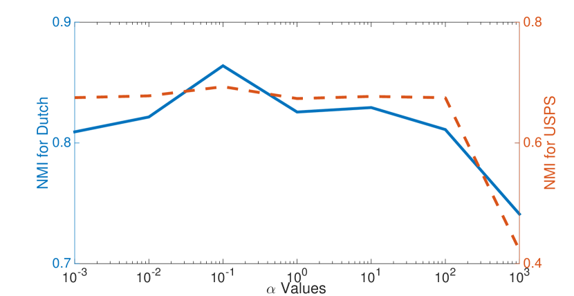
Figure 4: NMI v.s. $\alpha_{i}^{k}$ on Dutch-USPS.

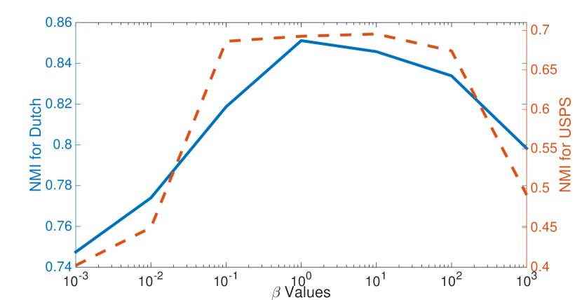
Figure 5: NMI v.s. $\beta^{(i,j)}$ on Dutch-USPS.

V Discussion

In this section, we aim at analyzing MMC more in detail in order to answer the following four questions:
(1) How does the difficulty of the clustering problem affect the performance of these methods?
(2) How does percentage of known mappings between sources affect the performance of MMC?
(3) How good is the inferred similarity mapping?
(4) How fast does MMC converge?

To show the performance for clustering problem with different difficulties, we apply MMC to Dutch-USPS data but with different number of clusters (2 to 10). The difficulty of the clustering problem increases as the number of clusters increases. The results are shown in Table V. The percentage of known mappings is also set to 60%. The NMIs for both sources are reported in separate rows (MMC(D) for Dutch and MMC(U) for USPS).

From Table V, we can observe that as the number of clusters increases (the difficulty of the problem increases), the performance for all of the methods decrease. The proposed MMC outperforms other comparison methods in almost all cases with one exception. CoReg-M outperforms MMC on USPS when the cluster number is 4. However, the proposed MMC achieved the second best performance in that case.

To answer the second question, we apply MMC on both Dutch-USPS data and English-Translation data with various percentages of known mapping between 30% to 100 % (10% interval). The results are shown in Tables VI and VII. It is worth noting that Sym-NMF, CoReg-S and MultiNMF-S do not utilize the instance mapping across sources. Thus, the performance of these three methods remain the same for different percentages.

In Table VI and Table VII, the proposed MMC outperforms the other comparison methods for both sources in almost all of the different parameter settings. It is important to notice that even with 100% mapping available, the proposed MMC is still better than other multi-view clustering methods. This is because MMC will treat views within one source as a cohesive set while other multi-view clustering algorithms treat the views from different sources equally.

TABLE VI: NMI for Dutch-USPS data with various percentages of known mapping

Method	30% known	40% known	50% known	60% known	70% known	80% known	90% known	100% known
Concat(D)	0.5515	0.5616	0.5631	0.5734	0.5770	0.5887	0.6064	0.6128
Sym-NMF(D)	0.7778	0.7778	0.7778	0.7778	0.7778	0.7778	0.7778	0.7778
MultiNMF-S(D)	0.5382	0.5382	0.5382	0.5382	0.5382	0.5382	0.5382	0.5382
MultiNMF-M(D)	0.6081	0.6676	0.7031	0.7585	0.8040	0.8130	0.7799	0.8356
CoReg-S(D)	0.7503	0.7503	0.7503	0.7503	0.7503	0.7503	0.7503	0.7503
CoReg-M(D)	0.7827	0.7861	0.7825	0.7886	0.8038	0.8343	0.8492	0.8596
CGC(D)	0.7947	0.7891	0.8019	0.7851	0.7929	0.7840	0.7878	0.8003
MMC(D)	0.7931	0.7903	0.8177	0.8248	0.8371	0.8537	0.8611	0.8746
Concat(U)	0.3067	0.3231	0.3623	0.3916	0.4354	0.4789	0.5350	0.6128
Sym-NMF(U)	0.3005	0.3005	0.3005	0.3005	0.3005	0.3005	0.3005	0.3005
MultiNMF-S(U)	0.401	0.4010	0.4010	0.4010	0.4010	0.4010	0.4010	0.4010
MultiNMF-M(U)	0.3468	0.3611	0.5029	0.4700	0.6007	0.6083	0.7011	0.7816
CoReg-S(U)	0.4044	0.4044	0.4044	0.4044	0.4044	0.4044	0.4044	0.4044
CoReg-M(U)	0.3527	0.4094	0.4607	0.5257	0.5808	0.6642	0.7541	0.8564
CGC(U)	0.2968	0.2902	0.2795	0.2780	0.2958	0.2882	0.2758	0.2898
MMC(U)	0.496	0.5463	0.6039	0.6348	0.6862	0.7587	0.8262	0.8684

TABLE VII: NMI for English-Translation data with various percentages of known mapping

Method	30% known	40% known	50% known	60% known	70% known	80% known	90% known	100% known
Concat(E)	0.1144	0.1334	0.1617	0.1914	0.2037	0.2488	0.2495	0.2498
Sym-NMF(E)	0.2783	0.2783	0.2783	0.2783	0.2783	0.2783	0.2783	0.2783
MultiNMF-S(E)	0.3413	0.3413	0.3413	0.3413	0.3413	0.3413	0.3413	0.3413
MultiNMF-M(E)	0.3253	0.3289	0.3339	0.3420	0.3689	0.3531	0.3523	0.3508
CoReg-S(E)	0.3381	0.3381	0.3381	0.3381	0.3381	0.3381	0.3381	0.3381
CoReg-M(E)	0.2060	0.2088	0.2098	0.2187	0.2194	0.2193	0.2184	0.2182
CGC(E)	0.2388	0.2550	0.2656	0.2636	0.2707	0.2680	0.2737	0.2740
MMC(E)	0.3436	0.3485	0.3571	0.3528	0.3576	0.3595	0.3558	0.3637
Concat(T)	0.1044	0.1124	0.1397	0.1621	0.1685	0.2098	0.2072	0.2198
Sym-NMF(T)	0.1527	0.1527	0.1527	0.1527	0.1527	0.1527	0.1527	0.1527
MultiNMF-S(T)	0.2708	0.2708	0.2708	0.2708	0.2708	0.2708	0.2708	0.2708
MultiNMF-M(T)	0.1945	0.2063	0.2146	0.2164	0.2146	0.2223	0.2541	0.2581
CoReg-S(T)	0.2874	0.2874	0.2874	0.2874	0.2874	0.2874	0.2874	0.2874
CoReg-M(T)	0.2160	0.2146	0.2178	0.2198	0.2171	0.2213	0.2210	0.2299
CGC(T)	0.2288	0.2450	0.2556	0.2536	0.2607	0.2580	0.2637	0.2640
MMC(T)	0.3028	0.3075	0.3072	0.3073	0.3090	0.3144	0.3196	0.3230

From the results, we can conclude that MMC works for various percentages of known mapping across sources. The reason why MMC performs better is not only because it appreciates the cohesiveness of the views, but also for every iteration, MMC tries to infer the instance similarity mapping between different sources. Although the instance similarity mapping is not as the same as the instance mapping, it provides extra information about the partially known instance mapping. Thus the inferred instance similarity mappings will help improve clustering in the next iteration.

To show how good the inference of similarity mapping is, we perform another set of experiments to measure the quality of the inferred similarity mappings among those not-aligned instances. For each not-aligned instance, we select the most similar instance mapped by the similarity mapping. Then we check if the two instances are in the same class. We test the accuracy for different number of clusters on Dutch-USPS data. Here the percentage of known instance mapping is set to 60%. We reported the number of instances that are not aligned by the known mapping, and the number of class matches by the inference of similarity mappings in Table VIII.

TABLE VIII: The inference accuarcy under differnet cluster numbers on Dutch-USPS

$c=2$ $c=4$ $c=6$ $c=8$ $c=10$ instances 160 320 480 640 800 matches 113 259 349 429 522 accuracy 0.7063 0.8094 0.7271 0.6703 0.6525

TABLE IX: The number of iterations until converge

% Known $30\%$ $40\%$ $50\%$ $60\%$ $70\%$ $80\%$ $90\%$ # iter 14 14 15 18 19 21 17

From Table VIII, we can clearly observe that when the number of clusters is 4, the inference of similarity mapping can get an accuracy as high as 0.8094. As the number of clusters increases, the accuracy of the inference drops. However, even with the number of clusters being as high as 10, we still get an accuracy of 0.6525 for the inference. To have a better understanding of the inferred similarity mapping, we plot the similarity mapping among the unmapped instances from the Dutch-USPS data with four clusters and 60% known mapping in Fig. 6. The instances are sorted by the class label for both sources (the first 80 instances belongs to class 1, the second 80 instances belong to class 2, etc,.) The X axis indicates the instances in Dutch, while the Y axis indicates the instances in USPS. From the figure, we can clearly see that there are four dark squares of width 80 on the diagonal line, which indicates that the same class of instances are more likely to be mapped together.

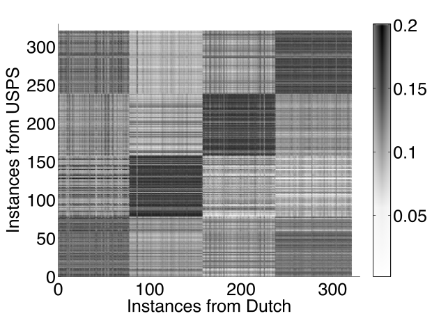
Figure 6: Scatter plot of the inferred similarity mapping for Dutch-USPS data with four clusters.

To show how fast MMC converges, we report the number of outer iterations until convergence for Dutch-USPS data in Table IX. From the table we can see that the method converges fast (less than 20 iterations).

VI Related Works

Multi-view learning [17, 3, 18, 4], is proposed to learn from instances which have multiple representations in different feature space. For example, [1] developed and studied partitioning and agglomerative, hierarchical multi-view clustering algorithms for text data. [3, 5] are among the first works proposed to solve clustering problem via spectral projection. [15] proposed to solve multi-view clustering by joint non-negative matrix factorization. [19, 6, 7, 20] are among the first works to solve the multi-view clustering with partial/incomplete views. However, none of the previous multi-view clustering methods can deal with incomplete and partial known mapping between sources/views. Further more, All the previous methods fail to treat the views within one source as a cohesive unit.

Consensus clustering [21, 22] is also related to the proposed MMC framework. It deals with the situation in which a number of different clustering results have been obtained for a particular dataset and it is desired to find a single consensus clustering which is a better fit in some sense than the existing ones. [23] gives a report about consensus clustering algorithms comparison and refinement. [24] proposes a bayesian consensus clustering method. However, consensus clustering aims to find a single consensus clustering from fully mapped clustering solutions. None of the previous methods works for the incomplete and partially unknown mappings between the instances.

VII Conclusion

This paper is the first to investigate the problem of clustering with multiple sources and multiple views. The proposed MMC framework treats views in the same source as a cohesive group for clustering by learning consensus latent feature matrices from the views within one source. It also incorporates multiple sources by using cross-source discrepancy penalty to enhance the clustering performance. MMC also uses the learned latent features to infer the cross-source unknown similarity mapping, which in turn will help improve the performance of clustering. Extensive experiments conducted on three groups of real-world data sets show the effectiveness of MMC comparing with other state-of-arts methods.

References

- [1] S. Bickel and T. Scheffer, “Multi-view clustering,” in ICDM, 2004.
- [2] K. Chaudhuri, S. M. Kakade, K. Livescu, and K. Sridharan, “Multi-view clustering via canonical correlation analysis,” in ICML, 2009.
- [3] A. Kumar, P. Rai, and H. D. III, “Co-regularized multi-view spectral clustering,” in NIPS, 2011.
- [4] B. Long, P. S. Yu, and Z. M. Zhang, “A general model for multiple view unsupervised learning.” in SDM. SIAM, 2008, pp. 822–833.
- [5] A. Kumar and H. D. III, “A co-training approach for multi-view spectral clustering,” in ICML, 2011.
- [6] W. Shao, X. Shi, and P. S. Yu, “Clustering on multiple incomplete datasets via collective kernel learning,” in ICDM, 2013.
- [7] S. Li, Y. Jiang, and Z. Zhou, “Partial multi-view clustering,” in AAAI, 2014, pp. 1968–1974.
- [8] W. Cheng, X. Zhang, Z. Guo, Y. Wu, P. F. Sullivan, and W. Wang, “Flexible and robust co-regularized multi-domain graph clustering.” in KDD, 2013.
- [9] W. Shao, L. He, and P. S. Yu, “Clustering on multi-source incomplete data via tensor modeling and factorization,” in PAKDD, 2015.
- [10] U. Luxburg, “A tutorial on spectral clustering,” Statistics and Computing, vol. 17, no. 4, pp. 395–416, Dec. 2007.
- [11] A. Y. Ng, M. I. Jordan, and Y. Weiss, “On spectral clustering: Analysis and an algorithm,” in NIPS, 2002, pp. 849–856.
- [12] X. Kong, J. Zhang, and P. S. Yu, “Inferring anchor links across multiple heterogeneous social networks,” in CIKM, 2013, pp. 179–188.
- [13] J. Zhang, P. S. Yu, and Z.-H. Zhou, “Meta-path based multi-network collective link prediction,” in KDD, 2014.
- [14] D. Kuang, H. Park, and C. H. Q. Ding, “Symmetric nonnegative matrix factorization for graph clustering.” in SDM, 2012, pp. 106–117.
- [15] J. Liu, C. Wang, J. Gao, and J. Han, “Multi-view clustering via joint nonnegative matrix factorization,” in SDM, 2013.
- [16] M. R. Amini, N. Usunier, and C. Goutte, “Learning from multiple partially observed views - an application to multilingual text categorization,” in NIPS, 2009.
- [17] A. Blum and T. Mitchell, “Combining labeled and unlabeled data with co-training,” in COLT, 1998.
- [18] K. Nigam and R. Ghani, “Analyzing the effectiveness and applicability of co-training,” in CIKM, 2000.
- [19] A. Trivedi, P. Rai, H. Daumé III, and S. DuVall, “Multiview clustering with incomplete views,” in NIPS Workshop, 2010.
- [20] W. Shao, L. He, and P. S. Yu, “Multiple incomplete views clustering via weighted nonnegative matrix factorization with regularization,” in ECML PKDD, 2015.
- [21] S. Monti, P. Tamayo, J. Mesirov, and T. Golub, “Consensus clustering: A resampling-based method for class discovery and visualization of gene expression microarray data,” Mach. Learn., 2003.
- [22] T. Li and C. Ding, “Weighted Consensus Clustering,” in SDM, 2008.
- [23] A. Goder and V. Filkov, “Consensus Clustering Algorithms: Comparison and Refinement,” in 9th Workshop on Algorithm Engineering and Experiments, 2008.
- [24] E. F. Lock and D. B. Dunson, “Bayesian consensus clustering.” Bioinformatics, vol. 29, no. 20, pp. 2610–2616, 2013.