A Catalog of Low-Mass Star-Forming Cores Observed with SHARC-II at 350 microns

Abstract

We present a catalog of low-mass dense cores observed with the SHARC-II instrument at 350 $\mu$m. Our observations have an effective angular resolution of 10^′′, approximately 2.5 times higher than observations at the same wavelength obtained with the Herschel Space Observatory, albeit with lower sensitivity, especially to extended emission. The catalog includes 81 maps covering a total of 164 detected sources. For each detected source, we tabulate basic source properties including position, peak intensity, flux density in fixed apertures, and radius. We examine the uncertainties in the pointing model applied to all SHARC-II data and conservatively find that the model corrections are good to within $\sim$3^′′, approximately $1/3$ of the SHARC-II beam. We examine the differences between two array scan modes and find that the instrument calibration, beam size, and beam shape are similar between the two modes. We also show that the same flux densities are measured when sources are observed in the two different modes, indicating that there are no systematic effects introduced into our catalog by utilizing two different scan patterns during the course of taking observations. We find a detection rate of 95% for protostellar cores but only 45% for starless cores, and demonstrate the existence of a SHARC-II detection bias against all but the most massive and compact starless cores. Finally, we discuss the improvements in protostellar classification enabled by these 350 $\mu$m observations.

1. Introduction

Stars form in dense cores of dust and molecular gas (e.g., Di Francesco et al., 2007; Ward-Thompson et al., 2007). The ultraviolet, optical, and infrared radiation from both stars forming inside cores and the interstellar radiation field (ISRF) is absorbed by the dust within these cores, heating the dust to typical temperatures of $10-20$ K (e.g., Di Francesco et al., 2007). The dust then re-radiates this emission at submillimeter and millimeter wavelengths. Thus, to study the very roots of star formation it is necessary to observe dense cores at these wavelengths.

Most nearby low-mass star-forming regions have been extensively surveyed at wavelengths between 850 $\mu$m and 1.3 mm due to the large number of bolometers available at these wavelengths and the high availability of weather suitable for $\sim$1 mm observations at most telescope sites (e.g., Motte et al., 1998; Testi & Sargent, 1998; Shirley et al., 2000; Johnstone et al., 2000, 2001; Motte & André, 2001; Motte et al., 2001; Young et al., 2003; Kirk et al., 2005; Enoch et al., 2006a; Stanke et al., 2006; Young et al., 2006a, b; Enoch et al., 2007a; Kauffmann et al., 2008). Because they are both optically thin and in the Rayleigh-Jeans limit for $10-20$ K dust, continuum observations at $\sim$1 mm are ideally suited for tracing the total dust mass and easily pick out the dense star-forming cores (e.g., Enoch et al., 2007a). However, since the peaks of $10-20$ K blackbodies occur at $250-500$ $\mu$m, these millimeter wavelength surveys do not constrain the peaks of the spectral energy distributions (SEDs). Observations at shorter submillimeter wavelengths are needed to measure total source luminosities (Dunham et al., 2008, 2013, 2014; Enoch et al., 2009a), separate the contributions from internal (from a protostar) and external (from the ISRF) heating (Dunham et al., 2006), and accurately classify protostars into an evolutionary sequence (Andre et al., 1993; Chen et al., 1995; Dunham et al., 2008, 2014; Frimann et al., 2015). Such observations are being provided by the Herschel Gould Belt Survey, which has obtained $70-500$ $\mu$m images of all of the nearby, star-forming clouds in the Gould Belt (e.g., André et al., 2010). While this survey is providing unprecedented coverage and sensitivity of nearby star-forming regions at submillimeter wavelengths, it is doing so at relatively low angular resolution (ranging from approximately 9^′′ at 70 $\mu$m to 36^′′ at 500 $\mu$m).

In an effort to provide a submillimeter catalog of dense cores with high spatial resolution, we present in this paper 350 $\mu$m continuum observations of low-mass protostellar cores taken with the Submillimeter High Angular Resolution Camera II (SHARC-II) at the Caltech Submillimeter Observatory (CSO) on Mauna Kea, Hawaii. SHARC-II was a 350 and 450 $\mu$m “CCD-style” bolometer array of 12 $\times$ 32 pixels giving an instantaneous field of view (FOV) of 2.59^′ $\times$ 0.97^′, with the pixels filling over 90% of the focal plane and separated by their projected size on the sky of 4.85^′′ (Dowell et al., 2003). With good focus and pointing, the 350 $\mu$m beam has a full-width at half-maximum (FWHM) of 8.5^′′. In practice the effective resolution at 350 $\mu$m is 10^′′ (see Section 3.1), providing 2.5 times higher angular resolution than the Herschel Gould Belt survey at the same wavelength (albeit at lower sensitivity, especially to extended emission). Targets were selected to provide complementary data to several large surveys of nearby, low-mass star-forming regions, including the Spitzer Space Telescope c2d (Evans et al., 2003, 2009) and Gould Belt (Gutermuth et al., 2008a; Dunham et al., 2015) Legacy Surveys and the Herschel Space Observatory DIGIT (e.g., Sturm et al., 2010; van Kempen et al., 2010; Green et al., 2013, 2016) open time Key Project. Some of the observations presented here were originally published by Wu et al. (2007), but we have re-analyzed and included them here using an updated version of the data reduction software and improved pointing model corrections. In general, we present observations of regions that are already well documented at other wavelengths so that this catalog will complement existing data in studies of the characteristics of protostellar regions. Though this is the primary goal of the paper, we also use our data to examine the sensitivity of SHARC-II to extended emission and to the observing mode used on the telescope, and to assess two different methods of classifying protostars.

We organize this paper as follows: First we describe the target selection and observation strategy in Sections 2.1 and 2.2, respectively. We then discuss the data reduction and calibration processes in Sections 3.1 and 3.2, respectively. We discuss the source extraction procedure in Section 3.3, including an analysis of the effects of optimizing the data reduction pipeline for the recovery of extended emission. We present our source catalog in Section 4, including source positions, flux densities, and radii. A comparison of the results from two different observing modes is presented in Section 5. In Section 6 we discuss the sensitivity of our observations to extended emission, and in Section 7 we investigate the effects of including SHARC-II 350 $\mu$m photometry when classifying protostars. A summary of our results is presented in Section 8.

2. Observations

2.1. Target Selection

Table 1 lists the targets of this survey, including the name of the core/cloud, the scan type (see below), the map center coordinates ordered by increasing Right Ascension, the distance to the target and reference for the distance determination, a representative reference for each target, the observation date, the 1$\sigma$ rms noise in units of mJy beam^-1, and the large cloud complex in which each target is located. As there is significant ambiguity in choosing a single representative reference for each target, we refer the reader to the SIMBAD database for a comprehensive list of references for each object. The noise is measured as the standard deviation of all off-source pixels, calculated using the sky procedure in the IDL Astronomy Library. Two versions of each map are produced, one with and one without extended emission preserved (see Section 3 below for details); the noise is measured in the maps without extended emission preserved.

As described in Section 1, the main purpose of this survey is to provide complementary 350 $\mu$m observations of low-mass star-forming clouds and cores observed in various Spitzer and Herschel survey programs. Thus targets were selected from the lists of regions included in those surveys, often focusing on individual studies that would benefit from these data. As a result, the data presented here do not represent an unbiased submillimeter survey of star-forming regions, but a targeted survey designed to provide a catalog of useful complementary data.

2.2. Observations

Observations were conducted at the CSO in 14 observing runs spread over seven years, ranging from May 2003 through December 2010. All of the data obtained between May 2003 and November 2005 were previously published (Wu et al. 2007); here we present updated images and catalogs using a newer version of the data reduction software (see Section 3). These data were obtained using the sweep mode of SHARC-II, which moves the telescope following Lissajous curves in both the x and y dimensions. This mode, which utilizes scan rates between 5–10 arcseconds s^-1 depending on the exact size mapped, results in a map with a fully sampled central region of uniform coverage, beyond which the coverage decreases and thus the noise increases. The size of this central region depends on the exact observing parameters, but is typically $\sim$ 1^′ $-$ 2^′ for our observations. Beginning in December 2006, we began experimenting with using the box-scan observing mode to map larger areas. This mode, which utilizes faster scan rates (typically in the range of 20–40 arcseconds s^-1), moves the telescope in a straight line at a 45^o angle until it hits the boundary of a box, changes direction such that the angle of reflection equals the angle of incidence, and continues until the box is fully sampled. The exact size of the box depends on the observing parameters, but is typically $\sim$ 6^′ $-$ 10^′ for our observations. As the box-scan mode is optimized for mapping both larger areas and regions with extended emission, all data obtained during and after July 2008 were obtained exclusively in this mode. Some sources were observed in both the Lissajous and box-scan observing modes. In those cases, only the box-scan observations are listed in Table 1. The Lissajous observations for these sources will be discussed in Section 5, where we compare results from the two observing modes.

The total integration time was typically $30-120$ minutes per map, depending on weather conditions and the expected brightness of sources in each map. The noise levels of the final maps span nearly two orders of magnitude, ranging from approximately 8 to 500 mJy beam^-1 (see below). Thus we caution that these maps form a very heterogeneous dataset in terms of sensitivity. Integrations for each map were broken into individual scans, each with a duration ranging from $5-15$ minutes depending on the stability of the atmosphere and the minimum time required to complete one scan in the chosen observing mode. The zenith optical depth at 225 GHz ranged from $0.03-0.09$, with values of $\sim 0.05-0.07$ most typical. With an approximate scaling factor of 20, these correspond to 350 $\mu$m zenith optical depths of $\sim 0.6-1.8$, with values of $\sim 1-1.4$ most typical. During all of our observations except those obtained in June 2005 (see Wu et al. 2007 for more details), the Dish Surface Optimization System (DSOS) was used to correct the dish surface figure for gravitational deformations as the dish moves in elevation during observations. The pointing and focus were both checked and updated every $1-2$ hr each night, primarily with the planets Mars, Uranus, and Neptune, but occasionally with other secondary calibrators chosen from the SHARC-II website. The pointing was further corrected in reduction based on a pointing model (see Section 3).

3. Data Reduction and Calibration

3.1. Data Reduction

The data were reduced using the Comprehensive Reduction Utility for SHARC-II (CRUSH) version 2.12-1, a publicly available, Java-based software package that iteratively solves for both the source signal and the various correlated noise components (e.g., Kovács, 2008a, b). For increased redundancy, we use CRUSH to add together the bolometer time streams from individual scans before obtaining the solutions, taking into account various noise elements and changing atmospheric conditions for each scan. The only exception to this general method is NGC1333, which had to be broken into five smaller pieces first due to computer memory limitations. These five pieces were then coadded together using the coadd function of the CRUSH package, after which point they were handled exactly the same way as the other sources. As described in more detail in Section 3.3 below, two versions of each map were produced: one with the extended flag given to CRUSH to optimize the software pipeline for the recovery of extended emission, and one without it given. The differences between and uses of the two versions of each map are discussed below.

The atmospheric opacity during each scan was determined from an online database of measurements of the zenith optical depth at 225 GHz, $\tau_{\rm 225GHz}$, obtained in ten minute intervals. This database includes polynomial fits to $\tau_{\rm 225GHz}$ versus time for each night, where the orders of the polynomials were treated as free parameters. The orders range from 3 to 90 over the full database, but are typically less than 20, with a mean value of 13. We visually inspected plots of $\tau_{\rm 225GHz}$ and the resulting polynomial fits for each night to verify that the fits accurately trace the variations in $\tau_{\rm 225GHz}$ throughout the night. CRUSH uses these polynomial fits to calculate the optical depth at the time each observation scan was taken and uses this value to correct the signal. Pointing corrections were applied to each scan with CRUSH to correct for residual telescope pointing errors. These corrections were determined using a publicly available model fit to all pointing data from that observing run. We applied this model using the option to also correct for a random drift with time by evaluating model residuals for pointing scans taken within a few hours before and after each science scan. The final maps were generated with 1.5^′′ pixels. A Gaussian smoothing function with a FWHM of 4 pixels was applied to each map to reduce pixelation artifacts, resulting in a final effective beam of approximately 10^′′.

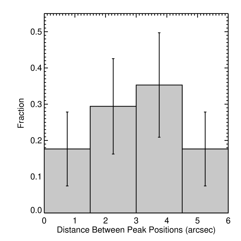
Figure 1.— Histogram of the distances between measured peak positions for several sources that were observed twice on two different dates, after applying the pointing model corrections.

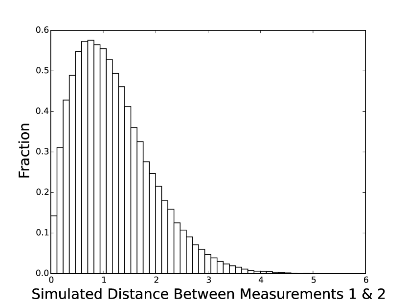
Figure 2.— Histogram showing the distance between measured peak positions for sources that were each observed twice in our Monte Carlo model, as explained in detail in the text. The mean distance is 1.2 and the median distance is 1.1 (both in arbitrary units). Since the model assumed a pointing rms of 1, we find that the mean of this distribution is 20% larger than the underlying rms of the pointing model.

In order to determine the residual pointing uncertainty after applying the pointing model corrections, Figure 1 shows a histogram of the distances between measured peak positions for several sources that were observed twice on two different dates, after applying the pointing model corrections. The mean distance is 2.9^′′. In order to interpret this in terms of a residual rms uncertainty in the pointing model, we construct a Monte Carlo model in which a source is placed on a polar coordinate grid twice, with each angle drawn randomly from a uniform distribution and each radius drawn randomly from a Gaussian distribtuion with $\sigma=1$. Note that this $\sigma$ has no units as we are only concerned with obtaining a dimensionless ratio that will characterize the pointing model uncertainty, as described below. The distribution of distances between the two “observations” of each source in the Monte Carlo model is shown in Figure 2; this distribution has a mean of 1.2. Since the input to the simulation was a pointing model with an assumed rms of 1, and the resulting mean of the distance distribution is 20% larger, we thus infer that our observed mean distance between peak positions of 2.9^′′ implies an underlying pointing model residual rms of 2.4^′′. Given the small number of sources observed twice and uncertainties in the assumptions of the Monte Carlo model, we thus conservatively estimate that the pointing model corrections are good to within $\sim 3^{\prime\prime}$.

Once the maps were created using CRUSH, we used the imagetool function of the CRUSH package to eliminate map edges with increased noise by removing all pixels in the map with less than 25% of the maximum integration time. The average 1$\sigma$ rms for each map was calculated by using the sky routine in the IDL Astronomy Library to measure the standard deviation of all off-source pixels and then calibrating with the peak calibration factor, as defined below.

3.2. Calibration

While CRUSH adopts an approximate calibration factor to produce maps in calibrated units of Jy beam^-1, it does not account for the fact that the instrument calibration changes both with observing conditions and randomly with time. Furthermore, the presence of beam sidelobes mean that the flux of a point source measured in apertures of increasing size will also increase, whereas ideally the flux of a point source should be independent of aperture size. We thus recalibrate all of our data as follows.

Figure 3.— Histograms for each set of calibration factors–peak, 20” aperture, and 40” aperture. The peak calibration factors are unitless. The 20” aperture and 40” aperture calibration factors convert from units of intensity (Jy beam^-1) to flux density (Jy) and therefore technically have units of Jy $/$ (Jy beam^-1) $=$ beam.

Figure 4.— Mean calibration factors for each observing run from 2003 to 2010. The error bars are the standard deviation from each run. The first, second, and third panels are the beam, 20” aperture, and 40” aperture respectively.

Figure 5.— Calibration factors from each planet scan plotted against the radius of the planet in that scan. The first, second, and third panels are the beam, 20” aperture, and 40” aperture respectively.

Figure 6.— Calibration factors from each planet scan plotted against the flux density of the planet in that scan. The first, second, and third panels are the beam, 20” aperture, and 40” aperture respectively.

To derive calibration factors, we used observations of Mars, Neptune, and Uranus, which were observed every few hours to check and update the telescope pointing. These planet scans, which we hereafter refer to as calibration scans, were reduced with CRUSH and used to calculate the calibration factors. All calibration scans were observed using the Lissajous observing mode on the telescope, regardless of what observing mode was used for the science sources to which these calibrations were applied. As shown in Section 5, the calibration factors do not depend on observing mode, validating this strategy. For each calibration scan, we measured the peak intensity and flux densities in 20^′′ and 40^′′ diameter apertures using custom IDL routines. We choose these aperture sizes to match previous (sub)millimeter continuum surveys that measure flux densities in standard apertures of 20^′′, 40^′′, 80^′′, and 120^′′ in diameter (e.g., Enoch et al., 2006a; Young et al., 2006b, a; Enoch et al., 2007a; Wu et al., 2007; Kauffmann et al., 2008). Here we only adopt the two smallest apertures since our calibration images are too small to use larger apertures. By comparing the measured flux densities to the known fluxes of these planets, we calculate three calibration factors: C_peak, C_20", and C_40". C_peak is simply the factor required to obtain calibrated maps in units of Jy beam^-1. Since the maps are already calibrated with an approximate calibration factor, the values of C_peak are unitless and are generally close to unity, as seen below. C_20" and C_40" are “aperture calibration factors” and have units of Jy / (Jy beam^-1) $=$ beam. Multiplying the flux densities measured through aperture photometry by the aperture calibration factors for the same size aperture will give the flux density in that aperture in Jy. As mentioned above, this method corrects for the beam sidelobes such that the measured flux density of a point source is independent of aperture size (e.g., Shirley et al., 2000; Enoch et al., 2006a).

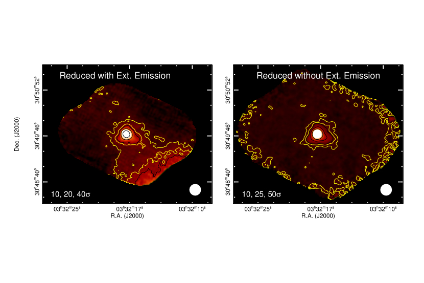
Figure 7.— IRAS 03292+3039 reduced with (left) and without (right) the extended emission flag included, with both panels displayed with a linear intensity color scale ranging from $-$0.4 to 3.0 Jy beam^-1 (see Figure 8 for a normalized version of the color scale bar used). The two yellow contours in each panel are plotted at 3$\sigma$ and 7$\sigma$, where 1$\sigma=0.55$ Jy beam^-1 in the map with the extended emission flag and 1$\sigma=0.15$ Jy beam^-1 in the map without the extended emission flag. Additional contours are plotted in black, with the levels chosen manually for optimal visual display and printed in white text in the lower left corner of each panel. The peak intensities (total flux densities in 40^′′ diameter apertures) are measured to be 9.6 Jy beam^-1 (17.4 Jy) in the map with the extended emission flag and 10.0 Jy beam^-1 (14.1 Jy) in the map without the extended emission flag.

In practice, C_peak, C_20", and C_40" are calculated as follows. For C_peak, the expected peak intensity from the planet was calculated by convolving the SHARC-II beam (assumed to be Gaussian) with a disk of uniform brightness, using the known size and flux density of each planet on that observation date. The resulting values are then divided by the measured peak intensity in each calibration scan. For C_20" and C_40", the known total flux density of the planet on each observation date was divided by the measured flux density in 20^′′ and 40^′′ diameter apertures, respectively, using the uncalibrated maps. The flux densities were measured using standard aperture photometry with no sky subtraction since CRUSH removes the background sky emission. Table 2 lists our derived calibration factors for each observation night, and Table 3 lists the means and standard deviations of the calibration factors for each observing run. Each map is calibrated using the mean calibration factors for that run; maps consisting of scans obtained over multiple runs are calibrated using the mean values over those runs. For maps observed in runs where no planet scans were taken, the mean calibration factors over all runs were used.

Figure 3 shows histograms for each of the calibration factors. To investigate whether the derived calibration factors vary with time or depend on the properties of the calibration source, Figures 4, 5, and 6 plot the calibration factors versus observation date, angular size of the calibration source, and total flux of the calibration source. No systematic variations are seen, and linear least squares fits to each panel in Figures 5 and 6 give better fits (lower reduced $\chi^{2}$ values) for zeroth order polynomial than for first order polynomials, indicating that any dependences of the calibration factors on source properties are smaller than the overall calibration uncertainties. We calculate these calibration uncertainties by dividing the standard deviations by the means, resulting in values of 18% for C_peak, 21% for C_20", and 17% for C_40". We thus conservatively adopt an overall calibration uncertainty of 25%.

3.3. Source Extraction

Figure 8.— Normalized intensity color scale bar for all of the images presented in this paper (Figures 7, 10–30, and 32–35). The minimum (black) and maximum (white) intensities for each map are presented in their respective figure captions.

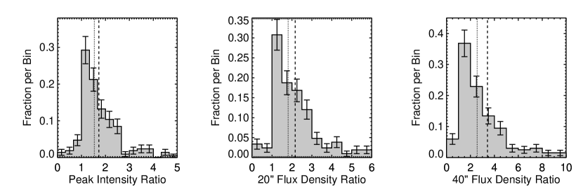
Figure 9.— Histograms for the ratios of flux densities measured in maps with the extended flag divided by those measured in maps without the extended flag, for each aperture size: The peak (beam) intensities (left), the flux densities in 20^′′ diameter apertures (middle), and the flux densities in 40^′′ diameter apertures (right). The vertical dashed lines in each panel shows the mean of each distribution, and the vertical dotted lines show the medians. The error bars on each bin are the statistical ($\sqrt{N}$) uncertainties.

As noted above, two versions of each map were produced, one with and one without the extended flag given to CRUSH. This flag optimizes the CRUSH pipeline for extended sources and results in maps that preserve extended emission at the cost of increased noise (see Kovács, 2008a, for details). Since our targets are star-forming regions expected to feature extended emission, we investigated the possibility of using this flag to recover more extended emission. However, we found that the added noise is dominated by sky noise that is temporally correlated in the time stream and thus spatially correlated in the final maps, rather than random, and thus especially problematic for source extraction. Many false sources are detected and extracted regardless of the detailed implementation of source extraction. Figure 7 shows an example of a map reduced with and without the extended flag. Similar color figures are presented for all of the regions mapped below. All maps are displayed with a linear intensity scaling with the minimum (black) and maximum (white) intensities given in their respective figure captions. Figure 8 displays a normalized intensity color scale bar that, combined with the minimum and maximum intensities given in the figure captions, can be used to determine the absolute intensities of each map.

Figure 7 illustrates that the extended flag results in large areas of correlated noise that are extracted as sources. Thus, in order to ensure a reliable catalog of sources, we perform source extraction on the maps produced without the extended flag (such as the one shown in the right panel of Figure 7). We extracted sources from each map using the Bolocat source extraction routine (Rosolowsky et al., 2010). Bolocat works by identifying regions of statistically significant emission based on their significance with respect to a local estimate of the noise in the maps. These regions of high significance are then subdivided into multiple sources based on the presence of local maxima within the originally defined regions, with each pixel assigned to one of the sources using a seeded watershed algorithm, similar to the Clumpfind or Source EXtractor algorithms (Williams et al., 1994; Bertin & Arnouts, 1996). Bolocat was previously used to extract sources from SHARC-II images of massive star-forming clumps by Merello et al. (2015), demonstrating the feasibility of using this source extraction routine on data from the SHARC-II instrument.

Bolocat requires three input parameters, all of which are measured in units of the map rms: $P_{\rm amp}$, the minimum required amplitude for a source to be extracted; $P_{\rm base}$, the base level of emission out to which the initial detected source is expanded; and $P_{\rm deb}$, a source deblending parameter. In practice, Bolocat first masks all regions of the map below $P_{\rm amp}$ and extracts one or more initial sources based on the number of regions of contiguous pixels remaining in the masked map. It then expands each of these initial sources to encompass all contiguous pixels down to the level $P_{\rm base}$, with the rationale being that marginally significant emission levels spatially connected to those of higher significance are likely to be real. Finally, each initial source is deblended into one or more sources by finding pairs of local maxima and identifying them as separate sources if the lower of the two is at least $P_{\rm deb}$ above the highest contour level that contains both maxima (see Rosolowsky et al., 2010, for details). We adopted values of $P_{\rm amp}=3$, $P_{\rm base}=3$, and $P_{\rm deb}=2$ based on matching “by-eye” extractions in an initial exploration of the parameter space (note that, since $P_{\rm amp}=P_{\rm base}$, we did not expand the sources beyond their initial detections). While Merello et al. (2015) also adopted $P_{\rm amp}=3$, they adopted lower values of the other two parameters ($P_{\rm base}=1$ and $P_{\rm deb}=1$). We found that the adoption of such low values for $P_{\rm base}$ and $P_{\rm deb}$ resulted in extractions that did not match either our best “by-eye” results or known sources from catalogs at other wavelengths. In particular, the lower value of $P_{\rm deb}$ resulted in several objects that were clearly single being broken into multiple objects due to small noise variations. The advantage of studying known regions with copious multiwavelength data in the literature, as opposed to Merello et al. (2015), allowed us to refine the best values of the source extraction parameters.

After extracting sources and measuring their deconvolved radii using the maps reduced without the extended flag, aperture photometry was performed on the maps produced with the extended flag, at the peak position of each extracted source. We used custom IDL routines to measure the peak intensities and flux densities in 20^′′ and 40^′′ diameter apertures. In cases of overlapping apertures with nearby sources, only those up to the largest in which overlap did not occur were kept. We measured the uncertainties in the flux densities in each aperture by adding in quadrature the statistical uncertainty from the measurement itself and the overall calibration uncertainty of 25%.

This method of using both sets of maps ensures that a reliable catalog of sources is extracted while also preserving as much extended emission as possible in the measured flux densities. Figure 9 shows the distribution of ratios of flux densities measured in the maps with the extended flag to those measured in the maps without the extended flag, for the peak intensities as well as the flux densities measured in 20^′′ and 40^′′ diameter apertures. The mean (median) ratios are 1.7 (1.5), 2.2 (1.8), and 3.4 (2.6) for the peak, 20^′′, and 40^′′ measurements. Thus, as expected, we see that the extended flag improves the flux recovery, especially in the larger apertures that are more sensitive to the amount of extended emission.

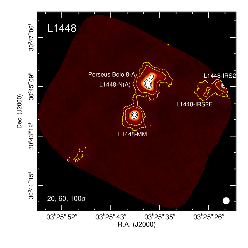
Figure 10.— SHARC-II 350 $\mu$m maps of the regions listed in Table 1, reduced without the extended emission flag and displayed on a linear intensity color scale, here L1448. Maps with multiple sources have each source labeled. The beam size is shown at the lower right of each map. The two yellow contour levels are plotted at 3$\sigma$ and 7$\sigma$, where 1$\sigma=0.151$ Jy beam^-1. Additional contours are plotted in black, with the levels chosen manually for optimal visual display. These levels are printed in white text at the bottom of each panel, with no text indicating no additional black contours are plotted. Emission seen toward the edges of the maps is not reliable and should be ignored. The color scaling uses a linear intensity scale ranging from $-$1.3 to 8.0 Jy beam^-1 (see Figure 8 for a normalized version of the adopted color scale bar).

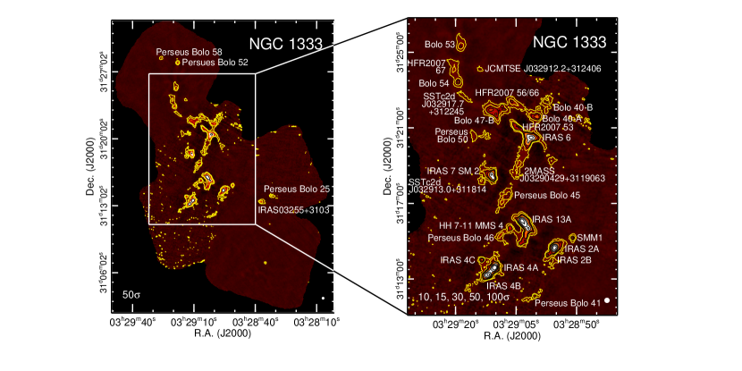
Figure 11.— Same as Figure 10, except for NGC1333 ($1\sigma$ = 0.170 Jy beam^-1, min = $-$1.2 Jy beam^-1, max = 5.8 Jy beam^-1). A few sources in the right panel are labeled as Bolo XX rather than Perseus Bolo XX to save space.

4. Results

Figures 10 – 30 show contour maps overlaid on images for each of the 81 regions listed in Table 1. Since the source extraction routine uses a local noise measurement but the contours are plotted using a global noise measurement, weak sources in low-noise regions may lack associated 3$\sigma$ contours. The images are of the maps reduced without the extended emission flag. Most maps are displayed in six-panel figures except for the largest and most crowded maps, which are instead displayed as one-panel figures. Maps with multiple sources have each source labeled. All of the reduced FITS files are available in calibrated units of Jy beam^-1 following the calibration procedures described above; versions with and without the extended flag can be accessed through the Data Behind the Figures (DBF) feature of the journal.

We detect a total of 164 sources in the 81 maps listed in Table 1 and presented in Figures 10 – 30. Table 4 lists, for each detected source, the name of the source, the map in which the source is covered, the peak position of the source, the deconvolved angular source radius as determined by Bolocat (see Rosolowsky et al., 2010, for details), the peak intensity, the flux density in a 20^′′ diameter aperture, the flux density in a 40^′′ diameter aperture, and a flag noting whether each source is starless or protostellar, determined mostly from a search for an infrared point source in Spitzer Space Telescope images from the c2d (e.g., Evans et al., 2009) and Gould Belt (e.g., Dunham et al., 2015) legacy projects. The peak intensities are given in units of Jy beam^-1 (for the SHARC-II beam, 1 Jy beam^-1 = 519.7 MJy sr^-1).

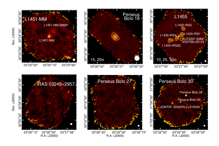
Figure 12.— Same as Figure 10, except for L1451-MM ($1\sigma$ = 0.089 Jy beam^-1, min = $-$0.1 Jy beam^-1, max = 0.7 Jy beam^-1), Perseus Bolo 18 ($1\sigma$ = 0.104 Jy beam^-1, min = $-$0.3 Jy beam^-1, max = 1.9 Jy beam^-1), L1455 ($1\sigma$ = 0.067 Jy beam^-1, min = $-$0.5 Jy beam^-1, max = 2.3 Jy beam^-1), IRAS 03249+2957 ($1\sigma$ = 0.105 Jy beam^-1, min = $-$0.1 Jy beam^-1, max = 0.9 Jy beam^-1), Perseus Bolo 27 ($1\sigma$ = 0.104 Jy beam^-1, min = $-$0.1 Jy beam^-1, max = 0.8 Jy beam^-1), and Perseus Bolo 30 ($1\sigma$ = 0.122 Jy beam^-1, min = $-$0.2 Jy beam^-1, max = 1.1 Jy beam^-1).

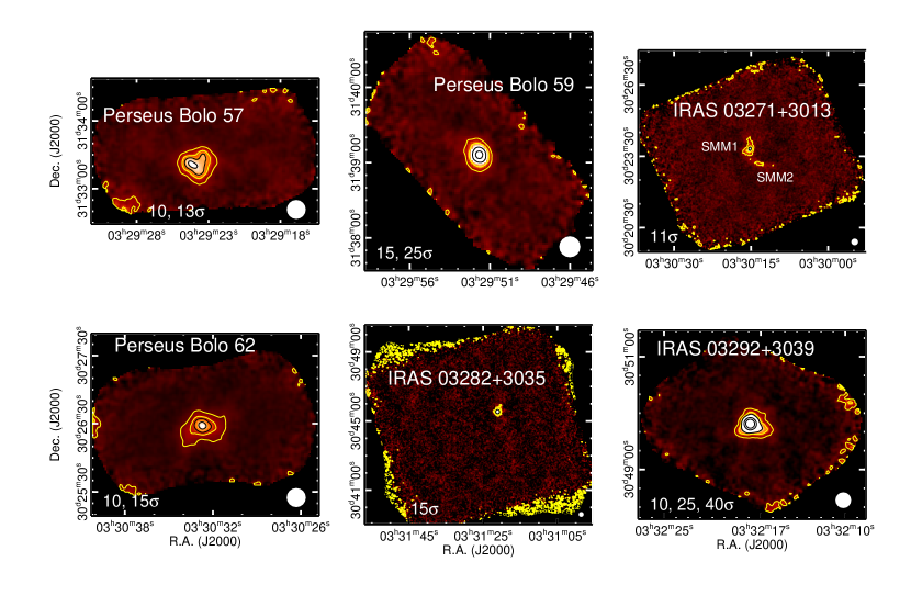
Figure 13.— Same as Figure 10, except for Perseus Bolo 57 ($1\sigma$ = 0.091 Jy beam^-1, min = $-$0.3 Jy beam^-1, max = 1.2 Jy beam^-1), Perseus Bolo 59 ($1\sigma$ = 0.114 Jy beam^-1, min = $-$0.3 Jy beam^-1, max = 1.2 Jy beam^-1), IRAS 03271+3013 ($1\sigma$ = 0.099 Jy beam^-1, min = $-$0.2 Jy beam^-1, max = 1.0 Jy beam^-1), Perseus Bolo 62 ($1\sigma$ = 0.044 Jy beam^-1, min = $-$0.1 Jy beam^-1, max = 0.7 Jy beam^-1), IRAS 03282+3035 ($1\sigma$ = 0.174 Jy beam^-1, min = $-$0.1 Jy beam^-1, max = 2.0 Jy beam^-1), and IRAS 03292+3039 ($1\sigma$ = 0.152 Jy beam^-1, min = $-$0.2 Jy beam^-1, max = 1.7 Jy beam^-1).

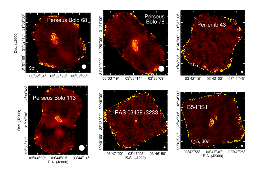
Figure 14.— Same as Figure 10, except for Perseus Bolo 68 ($1\sigma$ = 0.096 Jy beam^-1, min = $-$0.1 Jy beam^-1, max = 0.9 Jy beam^-1), Perseus Bolo 78 ($1\sigma$ = 0.111 Jy beam^-1, min = $-$0.2 Jy beam^-1, max = 0.8 Jy beam^-1), Per-emb 43 ($1\sigma$ = 0.083 Jy beam^-1, min = $-$0.1 Jy beam^-1, max = 0.6 Jy beam^-1), Perseus Bolo 113 ($1\sigma$ = 0.087 Jy beam^-1, min = $-$0.1 Jy beam^-1, max = 0.6 Jy beam^-1), IRAS 03439+3233 ($1\sigma$ = 0.176 Jy beam^-1, min = $-$0.1 Jy beam^-1, max = 0.5 Jy beam^-1), and B5-IRS1 ($1\sigma$ = 0.095 Jy beam^-1, min = $-$0.2 Jy beam^-1, max = 1.2 Jy beam^-1).

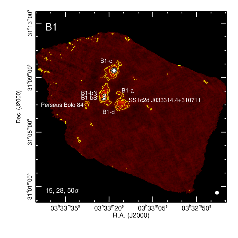
Figure 15.— Same as Figure 10, except for B1 ($1\sigma$ = 0.121 Jy beam^-1, min = $-$0.9 Jy beam^-1, max = 3.7 Jy beam^-1).

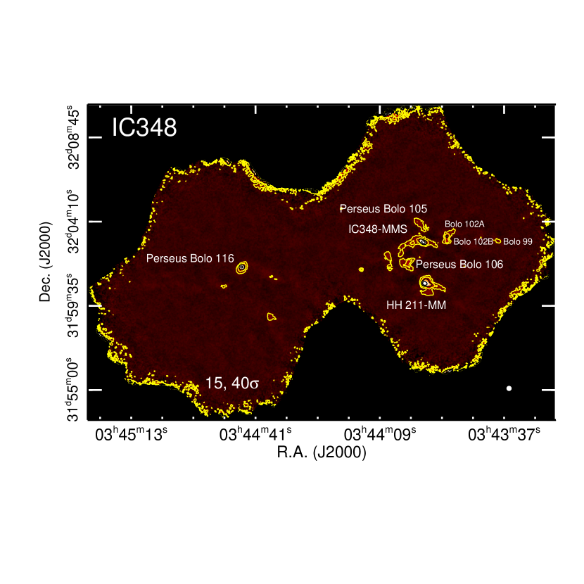
Figure 16.— Same as Figure 10, except for IC348 ($1\sigma$ = 0.121 Jy beam^-1, min = $-$0.6 Jy beam^-1, max = 3.3 Jy beam^-1).

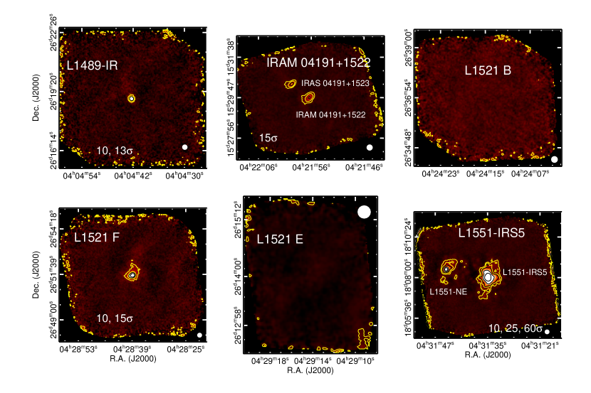
Figure 17.— Same as Figure 10, except for L1489-IR ($1\sigma$ = 0.153 Jy beam^-1, min = $-$0.3 Jy beam^-1, max = 0.2 Jy beam^-1), IRAM 04191+1522 ($1\sigma$ = 0.080 Jy beam^-1, min = $-$0.2 Jy beam^-1, max = 2.3 Jy beam^-1), L1521B ($1\sigma$ = 0.091 Jy beam^-1, min = $-$0.3 Jy beam^-1, max = 1.3 Jy beam^-1), L1521F ($1\sigma$ = 0.056 Jy beam^-1, min = $-$0.1 Jy beam^-1, max = 0.7 Jy beam^-1), L1521E ($1\sigma$ = 0.087 Jy beam^-1, min = 0.1 Jy beam^-1, max = 2.1 Jy beam^-1), and L1551-IRS5 ($1\sigma$ = 0.123 Jy beam^-1, min = $-$0.4 Jy beam^-1, max = 2.7 Jy beam^-1).

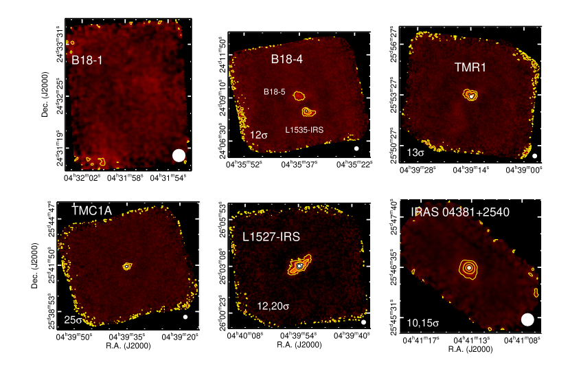
Figure 18.— Same as Figure 10, except for B18-1 ($1\sigma$ = 0.107 Jy beam^-1, min = $-$0.3 Jy beam^-1, max = 1.1 Jy beam^-1), B18-4 ($1\sigma$ = 0.073 Jy beam^-1, min = $-$0.3 Jy beam^-1, max = 1.2 Jy beam^-1), TMR1 ($1\sigma$ = 0.084 Jy beam^-1, min = $-$0.3 Jy beam^-1, max = 1.5 Jy beam^-1), TMC1A ($1\sigma$ = 0.114 Jy beam^-1, min = $-$0.4 Jy beam^-1, max = 2.3 Jy beam^-1), L1527-IRS ($1\sigma$ = 0.155 Jy beam^-1, min = $-$0.1 Jy beam^-1, max = 2.1 Jy beam^-1), and IRAS 04381+2540 ($1\sigma$ = 0.100 Jy beam^-1, min = $-$0.2 Jy beam^-1, max = 1.9 Jy beam^-1).

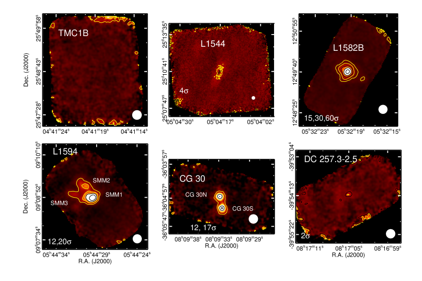
Figure 19.— Same as Figure 10, except for TMC1B ($1\sigma$ = 0.086 Jy beam^-1, min = $-$0.3 Jy beam^-1, max = 1.1 Jy beam^-1), L1544 ($1\sigma$ = 0.058 Jy beam^-1, min = $-$0.2 Jy beam^-1, max = 0.6 Jy beam^-1), L1582B ($1\sigma$ = 0.123 Jy beam^-1, min = $-$0.8 Jy beam^-1, max = 3.9 Jy beam^-1), L1594 ($1\sigma$ = 0.210 Jy beam^-1, min = $-$0.4 Jy beam^-1, max = 2.8 Jy beam^-1), CG 30 ($1\sigma$ = 0.452 Jy beam^-1, min = $-$0.4 Jy beam^-1, max = 4.3 Jy beam^-1), and DC 257.3-2.5 ($1\sigma$ = 0.067 Jy beam^-1, min = $-$0.2 Jy beam^-1, max = 0.6 Jy beam^-1).

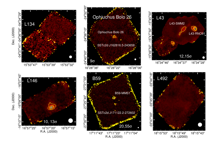
Figure 20.— Same as Figure 10, except for L134 ($1\sigma$ = 0.196 Jy beam^-1, min = $-$0.3 Jy beam^-1, max = 1.2 Jy beam^-1), Ophiuchus Bolo 26 ($1\sigma$ = 0.181 Jy beam^-1, min = $-$0.3 Jy beam^-1, max = 2.2 Jy beam^-1), L43 ($1\sigma$ = 0.194 Jy beam^-1, min = $-$0.6 Jy beam^-1, max = 2.9 Jy beam^-1), L146 ($1\sigma$ = 0.338 Jy beam^-1, min = $-$0.6 Jy beam^-1, max = 4.7 Jy beam^-1), B59 ($1\sigma$ = 0.319 Jy beam^-1, min = $-$0.4 Jy beam^-1, max = 5.0 Jy beam^-1), and L492 ($1\sigma$ = 0.052 Jy beam^-1, min = $-$0.2 Jy beam^-1, max = 1.1 Jy beam^-1).

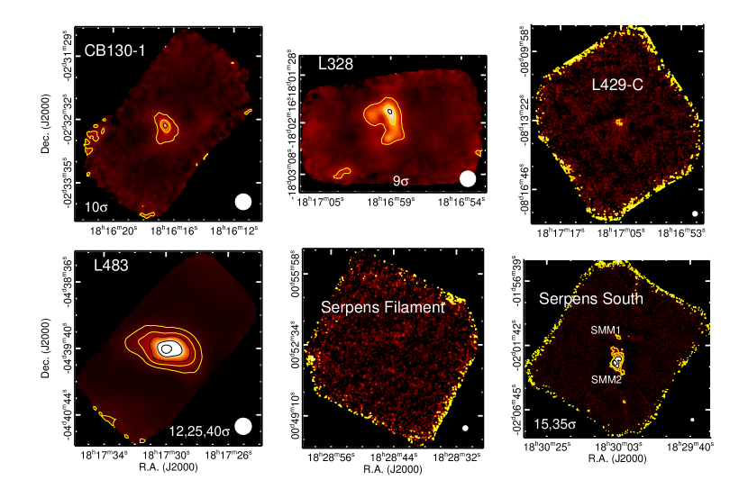
Figure 21.— Same as Figure 10, except for CB130-1 ($1\sigma$ = 0.069 Jy beam^-1, min = $-$0.1 Jy beam^-1, max = 1.0 Jy beam^-1), L328 ($1\sigma$ = 0.121 Jy beam^-1, min = $-$0.3 Jy beam^-1, max = 1.1 Jy beam^-1), L429-C ($1\sigma$ = 0.117 Jy beam^-1, min = $-$0.1 Jy beam^-1, max = 0.7 Jy beam^-1), L483 ($1\sigma$ = 0.251 Jy beam^-1, min = $-$0.6 Jy beam^-1, max = 6.3 Jy beam^-1), Serpens Filament ($1\sigma$ = 0.478 Jy beam^-1, min = $-$0.1 Jy beam^-1, max = 2.0 Jy beam^-1), and Serpens South ($1\sigma$ = 0.432 Jy beam^-1, min = $-$0.4 Jy beam^-1, max = 6.5 Jy beam^-1).

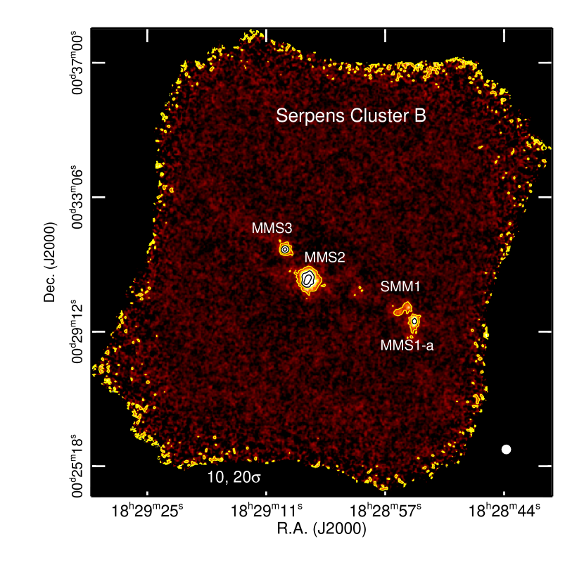
Figure 22.— Same as Figure 10, except for Serpens Cluster B ($1\sigma$ = 0.352 Jy beam^-1, min = $-$0.4 Jy beam^-1, max = 2.6 Jy beam^-1).

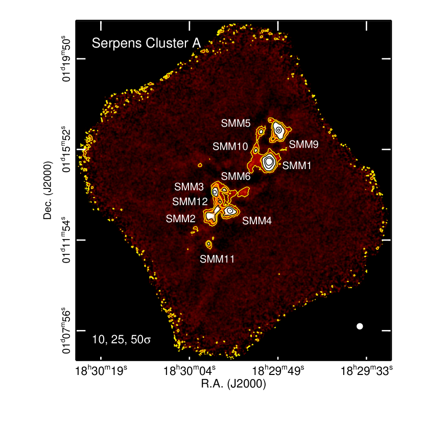
Figure 23.— Same as Figure 10, except for Serpens Cluster A ($1\sigma$ = 0.342 Jy beam^-1, min = $-$0.7 Jy beam^-1, max = 4.6 Jy beam^-1).

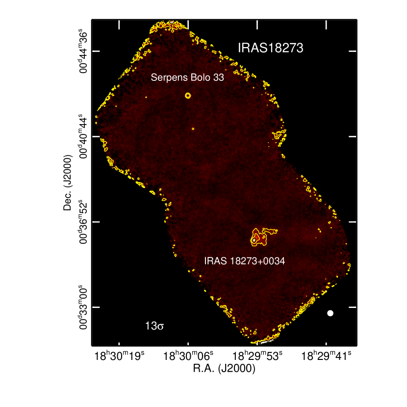
Figure 24.— Same as Figure 10, except for IRAS 18273 ($1\sigma$ = 0.101 Jy beam^-1, min = $-$0.3 Jy beam^-1, max = 2.2 Jy beam^-1).

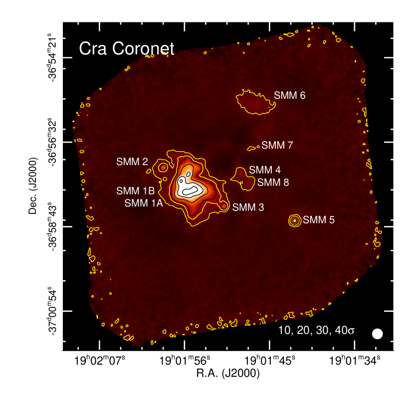
Figure 25.— Same as Figure 10, except for CrA Coronet ($1\sigma$ = 0.445 Jy beam^-1, min = $-$2.7 Jy beam^-1, max = 13.6 Jy beam^-1).

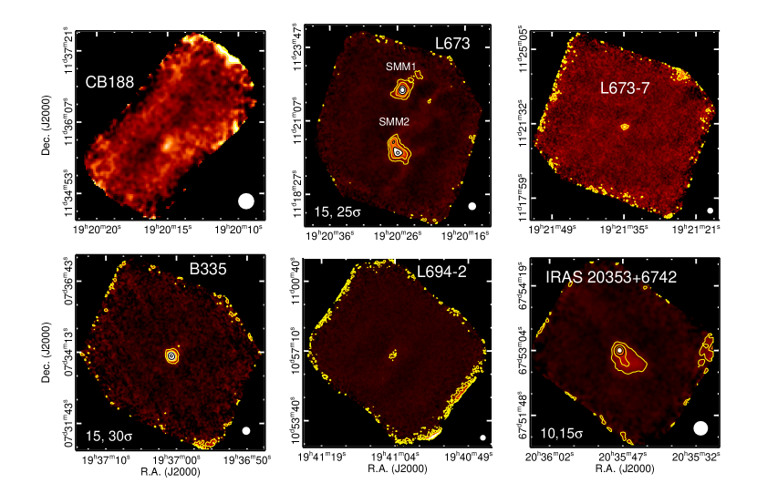
Figure 26.— Same as Figure 10, except for CB188 ($1\sigma$ = 0.261 Jy beam^-1, min = $-$0.4 Jy beam^-1, max = 0.9 Jy beam^-1), L673 ($1\sigma$ = 0.114 Jy beam^-1, min = $-$0.3 Jy beam^-1, max = 2.2 Jy beam^-1), L673-7 ($1\sigma$ = 0.083 Jy beam^-1, min = $-$0.3 Jy beam^-1, max = 0.7 Jy beam^-1), B335 ($1\sigma$ = 0.298 Jy beam^-1, min = $-$0.4 Jy beam^-1, max = 3.3 Jy beam^-1), L694-2 ($1\sigma$ = 0.078 Jy beam^-1, min = $-$0.3 Jy beam^-1, max = 2.2 Jy beam^-1), and IRAS 20353+6742 ($1\sigma$ = 0.105 Jy beam^-1, min = $-$0.2 Jy beam^-1, max = 2.0 Jy beam^-1).

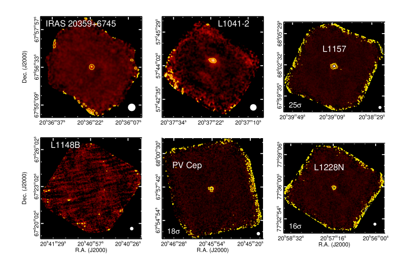
Figure 27.— Same as Figure 10, except for IRAS 20359+6745 ($1\sigma$ = 0.081 Jy beam^-1, min = $-$0.3 Jy beam^-1, max = 1.1 Jy beam^-1), L1041-2 ($1\sigma$ = 0.536 Jy beam^-1, min = $-$0.4 Jy beam^-1, max = 3.2 Jy beam^-1), L1157 ($1\sigma$ = 0.161 Jy beam^-1, min = $-$0.4 Jy beam^-1, max = 3.6 Jy beam^-1), L1148B ($1\sigma$ = 0.127 Jy beam^-1, min = $-$0.1 Jy beam^-1, max = 0.8 Jy beam^-1), PV Cep ($1\sigma$ = 0.242 Jy beam^-1, min = $-$0.4 Jy beam^-1, max = 3.5 Jy beam^-1), and L1228N ($1\sigma$ = 0.231 Jy beam^-1, min = $-$0.4 Jy beam^-1, max = 3.6 Jy beam^-1).

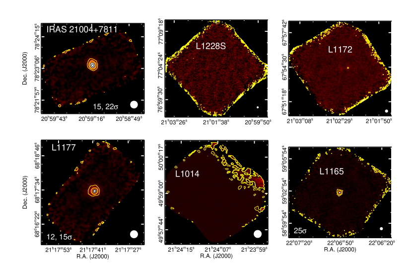
Figure 28.— Same as Figure 10, except for IRAS 21004+7811 ($1\sigma$ = 0.466 Jy beam^-1, min = $-$0.4 Jy beam^-1, max = 6.9 Jy beam^-1), L1228S ($1\sigma$ = 0.313 Jy beam^-1, min = $-$0.4 Jy beam^-1, max = 2.3 Jy beam^-1), L1172 ($1\sigma$ = 0.154 Jy beam^-1, min = $-$0.4 Jy beam^-1, max = 2.2 Jy beam^-1), L1177 ($1\sigma$ = 0.405 Jy beam^-1, min = $-$0.4 Jy beam^-1, max = 6.3 Jy beam^-1), L1014 ($1\sigma$ = 0.008 Jy beam^-1, min = $-$0.2 Jy beam^-1, max = 1.6 Jy beam^-1), and L1165 ($1\sigma$ = 0.163 Jy beam^-1, min = $-$0.3 Jy beam^-1, max = 4.7 Jy beam^-1).

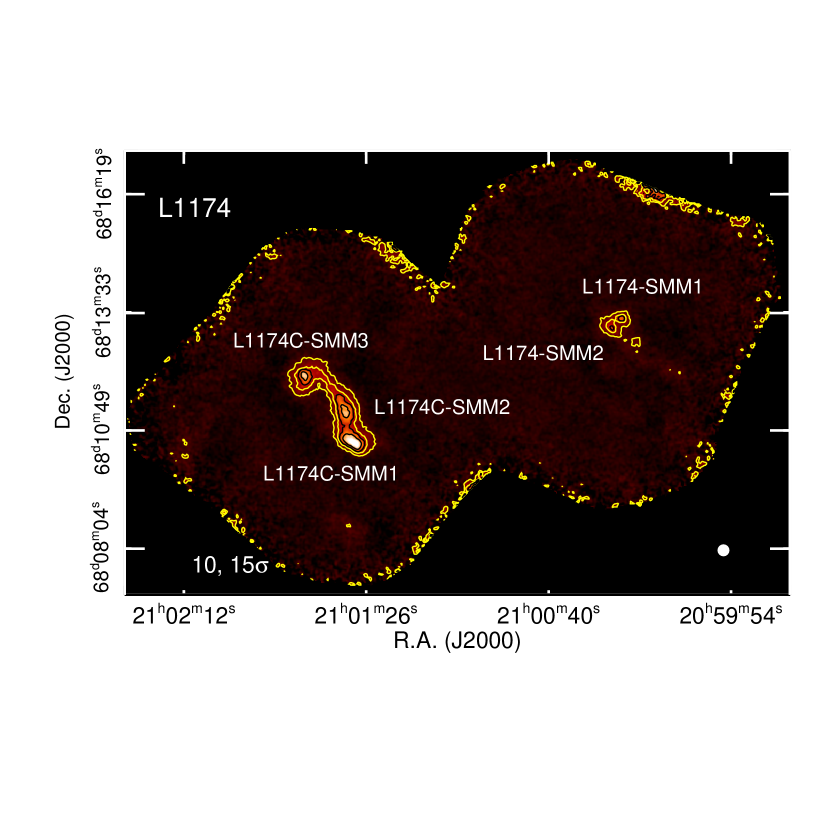
Figure 29.— Same as Figure 10, except for L1174 ($1\sigma$ = 0.141 Jy beam^-1, min = $-$0.3 Jy beam^-1, max = 2.9 Jy beam^-1).

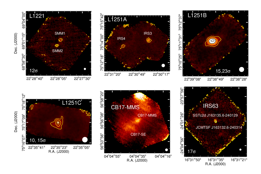
Figure 30.— Same as Figure 10, except for L1221 ($1\sigma$ = 0.250 Jy beam^-1, min = $-$0.4 Jy beam^-1, max = 3.7 Jy beam^-1), L1251A ($1\sigma$ = 0.144 Jy beam^-1, min = $-$0.4 Jy beam^-1, max = 2.8 Jy beam^-1), L1251B ($1\sigma$ = 0.278 Jy beam^-1, min = $-$0.5 Jy beam^-1, max = 4.4 Jy beam^-1), L1251C ($1\sigma$ = 0.240 Jy beam^-1, min = $-$0.8 Jy beam^-1, max = 4.9 Jy beam^-1), CB17-MMS ($1\sigma$ = 0.405 Jy beam^-1, min = $-$0.1 Jy beam^-1, max = 1.7 Jy beam^-1), and IRS63 ($1\sigma$ = 0.220 Jy beam^-1, min = $-$0.2 Jy beam^-1, max = 2.0 Jy beam^-1).

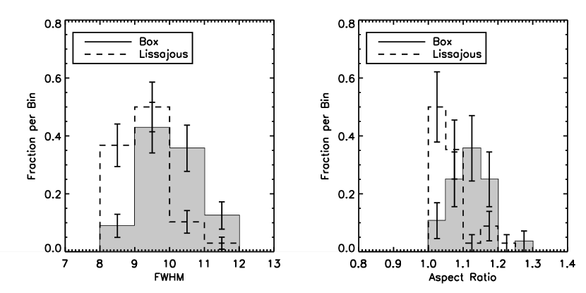
Figure 31.— Comparison of the FWHM (left) and aspect ratios (right) of the beams derived from the Lissajous (dashed histograms) and box (filled histograms) calibration scans.

5. Effects of Scan Mode

As noted in Section 2.2, all observations prior to 2006 were taken in the Lissajous scan mode. However, over the course of taking observations we were made aware of a different observing mode, the box scan mode, that might yield better results. In particular, maps observed in the box scan mode have much larger areas than those observed in the Lissajous mode. Since all emission on scales larger than the map size will be treated as sky emission and removed by CRUSH, the larger map areas provided by the box scans may provide better recovery of extended emission. The use of the box scan mode also allows us to map larger areas in reasonable amounts of time. Thus, all science data obtained during and after the July 2008 observing run were obtained exclusively in the box scan mode, with observations between December 2006 and July 2008 obtained in both modes for testing purposes.

Calibration scans were taken with the Lissajous mode, even after July 2008, since one Lissajous mode scan can be completed in much less time than one box scan. To justify this choice, we obtained several calibration scans in the box-scan observing mode. The calibration factors obtained from these scans are listed in Table 5, using the same method as above for the Lissajous calibration scans. Averaged over all of the box calibration scans, we calculate C${}_{\rm beam}=1.63\pm 0.15$, C${}_{\rm 20}=0.034\pm 0.004$, and C${}_{\rm 40}=0.025\pm 0.003$, where the uncertainties are the standard deviations. Comparison to Table 3 shows that the mean Lissajous and box-scan calibration factors agree to within 10%, well within the overall calibration uncertainty of 25%, indicating that any dependence on observing mode in the SHARC-II instrument calibration has a negligible impact on our results.

We also compared the SHARC-II beams resulting from the Lissajous and box scans. Figure 31 compares the size and shape of the beams derived from the Lissajous and box calibration scans. The beam profiles are derived by deconvolving the measured properties (sizes and elongations) of the calibration sources with their known, intrinsic properties. For the beam FWHM, the means and standard deviations of the means are 9.3^′′ $\pm$ 0.2^′′ for the Lissajous scans and 10.0^′′ $\pm$ 0.2^′′ for the box scans. For the beam aspect ratio, the means and standard deviations of the means are 1.06 $\pm$ 0.01 for the Lissajous scans and 1.12 $\pm$ 0.01 for the box scans. Thus, observations in the box scan mode have a beam profile that is, on average, 8% larger and 6% more elongated than observations in the Lissajous mode. While the degradation of the beam profile in the box scan mode is a statistically robust finding, resulting from both the faster scan rates used by the box scan modes and astrometric errors in the SHARC-II pixel plate scale that build up over larger scan areas, the overall effects are less than 10% and have no significant impact on our results.

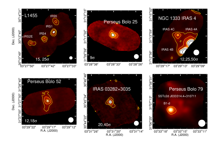
Figure 32.— SHARC-II 350 $\mu$m Lissajous maps of the targets listed in Table A Catalog of Low-Mass Star-Forming Cores Observed with SHARC-II at 350 microns (targets observed in both the Lissajous and box-scan observing modes), here L1455 ($1\sigma$ = 0.137 Jy beam^-1, min = $-$0.6 Jy beam^-1, max = 4.0 Jy beam^-1), Perseus Bolo 25 ($1\sigma$ = 0.040 Jy beam^-1, min = $-$0.2 Jy beam^-1, max = 0.6 Jy beam^-1), NGC 1333 IRAS 4 ($1\sigma$ = 0.341 Jy beam^-1, min = $-$0.6 Jy beam^-1, max = 4.8 Jy beam^-1), Perseus Bolo 52 ($1\sigma$ = 0.098 Jy beam^-1, min = $-$0.5 Jy beam^-1, max = 2.3 Jy beam^-1), IRAS 03282+3035 ($1\sigma$ = 0.169 Jy beam^-1, min = $-$0.6 Jy beam^-1, max = 5.0 Jy beam^-1), and Perseus Bolo 79 ($1\sigma$ = 0.358 Jy beam^-1, min = $-$0.2 Jy beam^-1, max = 3.1 Jy beam^-1). Maps with multiple sources have each source labeled. The beam size is shown at the lower right of each map. The two yellow contour levels are plotted at 3$\sigma$ and 7$\sigma$. Additional contours are plotted in black, with the levels chosen manually for optimal visual display. These levels are printed in white text at the bottom of each panel, with no text indicating no additional black contours are plotted. Emission seen toward the edges of the maps is not reliable and should be ignored. The color scaling uses a linear intensity scale; see Figure 8 for a normalized version of the adopted color scale bar.

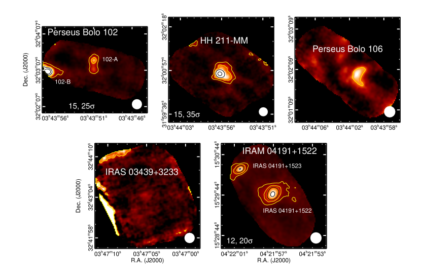
Figure 33.— Same as Figure 32 (Lissajous observations of targets observed in both models), except for Perseus Bolo 102 ($1\sigma$ = 0.195 Jy beam^-1, min = $-$0.3 Jy beam^-1, max = 2.5 Jy beam^-1), HH 211-MM ($1\sigma$ = 0.226 Jy beam^-1, min = $-$0.3 Jy beam^-1, max = 2.8 Jy beam^-1), Perseus Bolo 106 ($1\sigma$ = 0.287 Jy beam^-1, min = $-$0.3 Jy beam^-1, max = 1.3 Jy beam^-1), IRAS 03439+3233 ($1\sigma$ = 0.152 Jy beam^-1, min = $-$0.2 Jy beam^-1, max = 1.0 Jy beam^-1), and IRAM 04191+1522 ($1\sigma$ = 0.119 Jy beam^-1, min = $-$0.4 Jy beam^-1, max = 1.7 Jy beam^-1).

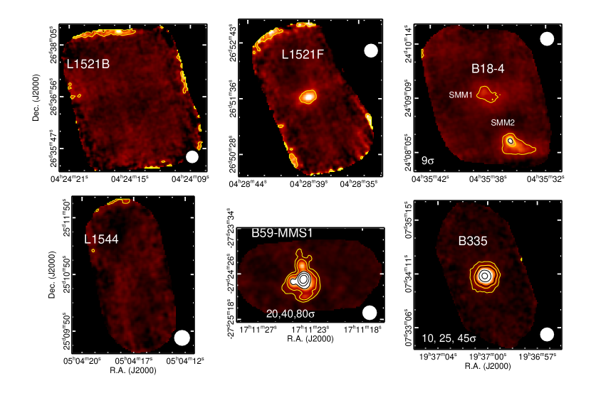
Figure 34.— Same as Figure 32 (Lissajous observations of targets observed in both models), except for L1521B ($1\sigma$ = 0.135 Jy beam^-1, min = $-$0.3 Jy beam^-1, max = 1.1 Jy beam^-1), L1521F ($1\sigma$ = 0.187 Jy beam^-1, min = $-$0.3 Jy beam^-1, max = 1.1 Jy beam^-1), B18-4 ($1\sigma$ = 0.120 Jy beam^-1, min = $-$0.3 Jy beam^-1, max = 1.2 Jy beam^-1), L1544 ($1\sigma$ = 0.071 Jy beam^-1, min = $-$0.1 Jy beam^-1, max = 0.9 Jy beam^-1), B59-MMS1 ($1\sigma$ = 0.200 Jy beam^-1, min = $-$0.6 Jy beam^-1, max = 4.2 Jy beam^-1), and B335 ($1\sigma$ = 0.223 Jy beam^-1, min = $-$0.5 Jy beam^-1, max = 4.4 Jy beam^-1).

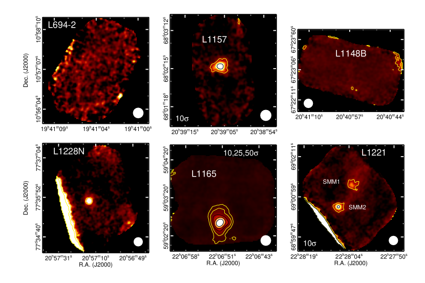
Figure 35.— Same as Figure 32 (Lissajous observations of targets observed in both models), except for L694-2 ($1\sigma$ = 0.257 Jy beam^-1, min = $-$0.3 Jy beam^-1, max = 1.1 Jy beam^-1), L1157 ($1\sigma$ = 0.631 Jy beam^-1, min = $-$0.3 Jy beam^-1, max = 5.0 Jy beam^-1), L1148B ($1\sigma$ = 0.063 Jy beam^-1, min = $-$0.3 Jy beam^-1, max = 1.2 Jy beam^-1), L1228N ($1\sigma$ = 1.023 Jy beam^-1, min = $-$0.3 Jy beam^-1, max = 4.8 Jy beam^-1), L1165 ($1\sigma$ = 0.087 Jy beam^-1, min = $-$0.4 Jy beam^-1, max = 3.9 Jy beam^-1), and L1221 ($1\sigma$ = 0.214 Jy beam^-1, min = $-$0.2 Jy beam^-1, max = 1.9 Jy beam^-1).

Figure 36.— Ratios of the flux densities calculated in maps observed in the box mode to those observed in the Lissajous mode, plotted versus the radius of each source determined from the box scan observations. The ratios of the peak intensities, flux densities in 20^′′ diameter apertures, and flux densities in 40^′′ diameter apertures are plotted in the left, middle, and right panels, respectively.

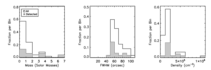
Figure 37.— Histograms showing the masses, FWHM, and mean densities of the starless cores identified in 1.1 mm Bolocam surveys of Perseus (Enoch et al., 2006a), Ophiuchus (Young et al., 2006b), and Serpens (Enoch et al., 2007a) and covered in our SHARC-II maps. The solid, unfilled histogram shows the properties of all (detected $+$ undetected) starless cores while the shaded histogram shows the properties of the starless cores detected in our SHARC-II survey.

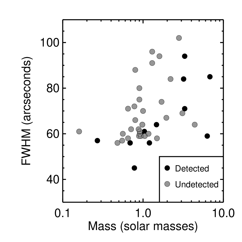
Figure 38.— FWHM size plotted versus mass for the starless cores identified in 1.1 mm Bolocam surveys of Perseus (Enoch et al., 2006a), Ophiuchus (Young et al., 2006b), and Serpens (Enoch et al., 2007a) and covered in our SHARC-II maps. The black points show those starless cores detected in our maps, whereas the light gray points show those cores that are not detected in our maps.

Figure 39.— $T_{bol}$ measured without 350 $\mu$m SHARC-II observations included in the SEDs plotted versus $T_{bol}$ measured with 350 $\mu$m SHARC-II observations included. The other data included in the SEDs used to calculate both values of $T_{bol}$ are at wavelengths between $3.6-70$ $\mu$m, and at 1.1 mm (see text for details). The solid line shows the one-to-one line, and the dashed line marks the Class 0/I boundary in $T_{bol}$ as defined by Chen et al. (1995).

Figure 40.— $L_{smm}/L_{bol}$ plotted versus $T_{bol}$, in both cases measured with 350 $\mu$m SHARC-II observations included in the SEDs. The other data included in the SEDs used to calculate both values are the same as in Figure 39. The vertical dashed lines show the Class boundaries in $T_{bol}$ as defined by Chen et al. (1995), and the horizontal dashed lines show the Class boundaries in $L_{smm}/L_{bol}$ as defined by Andre et al. (1993).

Finally, we also investigated whether the measured flux densities of our science targets depended on the observing mode. To do this, we observed several science sources in both observing modes. For the 23 maps observed in both modes, Tables 1 and 4 only present information for the box scans; the target and source information for the Lissajous scans are given in Tables A Catalog of Low-Mass Star-Forming Cores Observed with SHARC-II at 350 microns and 7. We extracted sources from these extra Lissajous maps and measured flux densities using the same methods as described above. Figures 32 – 35 show contour maps overlaid on images for these extra Lissajous maps, using the maps reduced without the extended emission flag. All of the reduced FITS files used to produce these figures are available through the Data Behind the Figures (DBF) feature of the journal. These maps are given in calibrated units of Jy beam^-1 following the calibration procedures described above, and both the versions with and without the extended flag are provided. For the sources detected in both modes, Figure 36 plots the ratios of the flux densities calculated in maps observed in the box mode to those observed in the Lissajous mode versus the radius of each source determined from the box scan observations. The means and standard deviations of these ratios are $0.93\pm 0.18$, $0.97\pm 0.17$, and $1.09\pm 0.29$ for the peak intensities, 20^′′ flux densities, and 40^′′ flux densities, respectively. In all three cases the mean ratios are within 10% of unity. Given the overall calibration uncertainty of 25% and the fact that the ratios show no dependence on source radius, we conclude that similar amounts of flux are recovered between the two observing modes on scales up to at least 40^′′.

6. Sensitivity to Extended Emission

In addition to the detected sources listed in Table 4, Table 8 lists an additional 48 cores covered by our maps but not detected in our SHARC-II observations. These are cores identified by other observations at submillimeter and millimeter wavelengths, based on SIMBAD searches of the total area covered by our maps. Combining the information from these tables, our maps cover a total of 137 protostellar cores, 130 of which are detected, and a total of 75 starless cores, 34 of which are detected. Our detection rate of 95% for protostellar cores is thus much higher than our detection rate of 45% for starless cores. These results suggest that SHARC-II is well suited for identifying and characterizing protostellar cores, but is not ideal for studying starless cores.

Of the maps observed in both the Lissajous and box scan modes, there are six starless cores. Two are detected in both modes (L1455-IRS2E and B18-4), two are detected in only the box scan mode (L1544 and L694-2), and two are undetected in both observing modes (Perseus Bolo 107 and L1521B). The lower detection rate for starless cores in the Lissajous mode (33%) versus the box scan mode (45%), coupled with the fact that two starless cores detected in the box scan mode are not detected in the Lissajous mode, suggest that the box scan mode is somewhat better suited to detecting starless cores, although we caution that the sample sizes are very small.

The low detection rate for starless cores is likely explained by the fact that, compared to protostellar cores, starless cores feature flatter density profiles and colder temperatures in their central regions (e.g., Ward-Thompson et al., 2007; Evans et al., 2001). Consequently starless cores exhibit 350 $\mu$m intensity profiles that are significantly shallower and less centrally condensed than those for protostellar sources, as confirmed by Wu et al. (2007) using simple, one-dimensional radiative transfer models. The more extended nature of their emission profiles make them harder to separate from sky emission, thus they are less reliably detected. To further quantify this effect, we examined all of the starless cores covered by our maps that were identified in 1.1 mm Bolocam surveys of Perseus (Enoch et al., 2006a), Ophiuchus (Young et al., 2006b), and Serpens (Enoch et al., 2007a). Figure 37 shows histograms of the core masses, sizes, and mean densities, as derived from the Bolocam observations, for both the detected and undetected populations of starless cores in our dataset. The detected starless sources span nearly the full range of masses, FWHM angular sizes, and mean densities, indicating there is no one unique property that determines the detectability of the core.

Figure 38 plots the FWHM angular size versus core mass for these same starless cores, again taking the properties from the 1.1 mm Bolocam surveys cited above. Inspection of this figure shows that, for low-mass cores ($M<\sim$2 M_⊙), only the most compact cores are detected. These cores will have the steepest intensity profiles among all cores with such masses, allowing them to be separated from sky emission and reliably detected. Only for relatively high-mass (and thus relatively bright) cores ($M>\sim$3 M_⊙) are more extended cores able to be separated from sky emission and detected by SHARC-II observations. Thus, starless cores revealed by SHARC-II surveys of star-forming regions are biased toward the most compact or highest mass cores, and even in cases where starless cores are detected, the extended nature of their intensity profiles means that the measured flux densities are likely lower limits to the true flux densities. These cautions should be kept in mind when interpreting the results from Zhang et al. (2015), who derive a prestellar core mass function based on SHARC-II observations of Ophiuchus. This core mass function for detected prestellar cores may not be representative of the full population of such cores in this cloud, and furthermore the measured masses of the detected prestellar cores likely underestimate their true masses. Since the detectability of a starless core with SHARC-II is not a simple function of the total flux density of the core, but also its emission profile, measured upper limits for undetected cores do not necessarily represent true limits to the flux densities of these cores. While we do list the 1$\sigma$ upper limits in Table 8 (taken directly from Table 1), this caution should be kept in mind when interpreting the non-detections.

While we caution that the measured flux densities of starless cores are likely lower limits, the measured values for the protostellar cores are much more reliable. Wu et al. (2007) used simple, one-dimensional radiative transfer models to show that protostellar cores exhibit significantly steeper intensity profiles compared to starless cores, even for protostars with luminosities as low as 0.1 L_⊙. These steeper intensity profiles lead to more compact emission that is fully recovered by SHARC-II, at least on scales up to the 40^′′ considered here. This is confirmed by comparing the SHARC-II observations of IRAM 04191+1522 and L1521F, two protostars with luminosities less than 0.1 L_⊙, to published radiative transfer models; in both cases the observed flux densities in 40^′′ diameter apertures agree with the models to within 2$\sigma$ (Dunham et al., 2006; Bourke et al., 2006a).

7. Classification of Protostars

Protostars are commonly classified into one of two classes, Class 0 and Class I, based on observational signatures that trace the underlying evolutionary state. Class 0 protostars were first defined by Andre et al. (1993), who defined such objects observationally as protostars emitting a relatively large fraction (greater than 0.5%) of their total luminosity at wavelengths $\lambda\geq 350$ $\mu$m. Defining such luminosity as the submillimeter luminosity, $L_{smm}$, Class 0 objects are then protostars with $L_{smm}/L_{bol}$ $>$ 0.005. The corresponding physical Stage 0 objects are young, embedded protostars with greater than 50% of their total system mass still in the core (Andre et al., 1993). Another quantity used to classify protostars is the bolometric temperature $T_{bol}$, defined by Myers & Ladd (1993) as the temperature of a blackbody with the same flux-weighted mean frequency as the source. By calculating $T_{bol}$ for a large sample of young stars, Chen et al. (1995) showed that Class 0 objects have $T_{bol}$ $<$ 70 K whereas Class I protostars have $T_{bol}$ $\geq$ 70 K. Since $L_{smm}$ has historically been difficult to calculate accurately due to the difficulty in obtaining high-quality submillimeter data from the ground, particularly at 350 $\mu$m, the $T_{bol}$ criterion introduced by Chen et al. is often used instead for classifying protostars into their two Classes (e.g., Enoch et al., 2009a; Dunham et al., 2013; Tobin et al., 2016). However, as several studies have shown that $L_{smm}/L_{bol}$ is less sensitive to viewing geometry and a better tracer of underlying physical stage than $T_{bol}$ (Andre et al., 2000; Young & Evans, 2005; Dunham et al., 2010b; Frimann et al., 2015), protostellar classification must be revisited as additional data becomes available.

With the 350 $\mu$m photometry presented here, we can now accurately calculate (to within 20%–60%; see Dunham et al., 2008; Enoch et al., 2009a, for details) both $T_{bol}$ and $L_{smm}/L_{bol}$ and compare classification via the two quantities. To ensure as uniform a dataset as possible, we consider only the protostellar cores in Perseus, and construct SEDs for each source consisting of Spitzer Space Telescope 3.6–70 $\mu$m photometry from Evans et al. (2009) and Dunham et al. (2015) and Bolocam 1.1 mm photometry from Enoch et al. (2006a). We calculate $T_{bol}$ twice, once without the SHARC-II 350 $\mu$m photometry included and once with it included, and we also calculate $L_{smm}/L_{bol}$.

Figure 39 compares the two values of $T_{bol}$, calculated with and without the 350 $\mu$m photometry included. Leaving out the 350 $\mu$m photometry increases the value of $T_{bol}$, with the effect growing in significance with decreasing evolutionary stage (colder values of $T_{bol}$). This result is explained by the fact that, for more deeply embedded protostars, the emission peaks at longer wavelengths, and more of this emission is lost when no submillimeter photometry is available. As demonstrated by Figure 39, Class 0 protostars with very low values of $T_{bol}$ can masquerade as more evolved objects when 350 $\mu$m photometry is lacking. These results are in qualitative agreement with earlier investigations by Dunham et al. (2008) and Enoch et al. (2009a).

Figure 40 plots $L_{bol}/L_{smm}$ versus $T_{bol}$ for these same protostars as a way of comparing the two different classification methods. Such a comparison is only possible when 350 $\mu$m data is available, since accurate calculation of $L_{smm}$ requires 350 $\mu$m data. With the $T_{bol}$ Class boundaries as defined by Chen et al. (1995) and the $L_{smm}/L_{bol}$ Class boundaries as defined by Andre et al. (1993), the two classification methods agree for only 65% of the protostars considered (35 out of 54). In particular, there are many protostars classified as Class I by $T_{bol}$ ($T_{bol}$ $>$ 70 K) but Class 0 by $L_{smm}/L_{bol}$ ($L_{smm}/L_{bol}$ $>$ 0.005). Revised $L_{smm}/L_{bol}$ Class 0/I boundaries have been proposed in the literature, including 0.01 (Andre et al., 2000; Sadavoy et al., 2014) and 0.03 (Maury et al., 2011). Adopting these boundaries increases the agreement between classification methods to 67% and 74%, respectively.

While the primary focus of this publication is to provide a catalog of SHARC-II 350 $\mu$m observations of nearby star-forming regions, these results demonstrate the critical role played by 350 $\mu$m observations in both accurate classification of protostars and assessing the reliability of different classification methods in tracing the underlying evolutionary stages of protostars. A more complete investigation of protostellar classification, using complete far-infrared and submillimeter SEDs provided by both ground-based surveys such as this effort and surveys with the Herschel Space Observatory, will be presented in a future paper (M. M. Dunham et al., in preparation).

8. Summary

In this paper we have presented a catalog of low-mass star-forming cores observed with the SHARC-II instrument at 350 $\mu$m. Our observations have an effective angular resolution of 10^′′, approximately three times higher than observations at the same wavelength obtained with the Herschel Space Observatory. A summary of our results is as follows:

• We present 81 maps covering a total of 164 detected sources. We tabulate basic source properties including position, peak intensity, flux density in fixed apertures, and radius.

• We examine the uncertainties in the pointing model applied to all SHARC-II data and conservatively find that the model corrections are good to within $\sim$3^′′, approximately $1/3$ of the SHARC-II beam.

• We examined the differences between the Lissajous and box scan observing modes. We find that the calibration factors, beam size, and beam shape are similar between the two modes, and we also show that the same flux densities are measured when sources are observed in the two different modes. Thus we conclude that there are no systematic effects in our catalog introduced by switching observing modes during the course of taking observations.

• We find that less than half of the starless cores observed are detected by SHARC-II (45% to be precise), and show that the detections are biased toward the most compact or highest mass starless cores. We argue that, even for the detected starless cores, the measured flux densities are likely lower limits to the intrinsic flux densities.

• For protostellar cores, our SHARC-II observations fully recover the emission, at least up to the 40^′′ scales considered here.

• We demonstrate that the inclusion of 350 $\mu$m photometry significantly improves the accuracy of calculated values of $T_{bol}$, and enables comparison between two different measures of protostellar Class, $T_{bol}$ and $L_{smm}/L_{bol}$. The latter can only be calculated when 350 $\mu$m photometry is available.

Table 1Observing Information

		Map Center	Map Center				1$\sigma$ Noise
	Scan	R.A.	Decl.	Dist.	Dist.	Source	Obs.	(mJy
Core/Cloud	Type	(2000.0)	(2000.0)	(pc)	Ref.	Ref.	Date	beam-1)	Cloud
L1451-mm	B	03 25 10.2	+30 23 55.0	250	1	1	2010 Dec	89	P
L1448	B	03 25 38.9	+30 44 05.4	250	1	2	2008 Oct	151	P
Perseus Bolo 18	L	03 26 37.5	+30 15 28.1	250	1	3	2007 Oct	104	P
L1455	B	03 27 41.0	+30 12 45.0	250	1	2	2007 Oct	67	P
IRAS 03249+2957	B	03 28 00.4	+30 08 01.3	250	1	4	2008 Oct	105	P
Perseus Bolo 27	B	03 28 33.3	+30 19 35.0	250	1	3	2009 Dec	104	P
Perseus Bolo 30	B	03 28 39.1	+31 06 01.8	250	1	3	2007 Oct	122	P
NGC1333	B	03 28 58.0	+31 17 30.0	250	1	2	2008 Oct; 2009 Sep	170	P
Perseus Bolo 57	L	03 29 23.4	+31 33 29.5	250	1	3	2007 Oct	91	P
Perseus Bolo 59	L	03 29 51.8	+31 39 06.1	250	1	3	2007 Oct	114	P
IRAS 03271+3013	B	03 30 14.9	+30 23 36.9	250	1	5	2009 Dec	99	P
Perseus Bolo 62	L	03 30 32.7	+30 26 26.2	250	1	3	2006 Dec	44	P
IRAS 03282+3035	B	03 31 26.0	+30 44 35.0	250	1	6	2008 Oct	174	P
IRAS 03292+3039	L	03 32 18.0	+30 49 47.0	250	1	7	2005 Nov	152	P
Perseus Bolo 68	L	03 32 28.1	+31 02 17.5	250	1	3	2005 Nov	96	P
B1	B	03 33 10.0	+31 06 14.0	250	1	2	2008 Oct; 2009 Sep, Dec	121	P
Perseus Bolo 78	L	03 33 13.8	+31 20 05.2	250	1	3	2007 Oct	111	P
Per-emb 43	B	03 42 02.2	+31 48 02.1	250	1	8	2009 Dec	83	P
Perseus Bolo 113	L	03 44 21.4	+31 59 32.6	250	1	3	2007 Oct	87	P
IC348	B	03 44 22.0	+32 02 30.0	250	1	2	2009 Sep	121	P
IRAS 03439+3233	B	03 47 05.4	+32 43 08.4	250	1	9	2009 Dec	176	P
B5-IRS1	B	03 47 40.8	+32 51 57.2	250	1	10	2009 Dec	95	P
CB17-MMS	B	04 04 35.8	+56 56 03.2	250	2	11	2010 Dec	405	I
L1489-IR	B	04 04 42.9	+26 18 56.3	140	3	12	2008 Oct	153	T
IRAM 04191+1522	B	04 21 56.9	+15 29 45.0	140	3	13	2007 Oct	80	T
L1521B	B	04 24 14.9	+26 36 53.0	140	3	14	2007 Oct	91	T
L1521F	B	04 28 38.9	+26 51 35.0	140	3	15	2006 Dec	56	T
L1521E	L	04 29 13.6	+26 14 05.0	140	3	14	2005 Nov	87	T
L1551-IRS5	B	04 31 34.1	+18 08 04.9	140	3	14	2009 Sep	123	T
B18-1	L	04 31 57.7	+24 32 30.0	140	3	14	2005 Nov	107	T
B18-4	B	04 35 37.5	+24 09 20.0	140	3	14	2007 Oct	73	T
TMR1	B	04 39 13.9	+25 53 20.6	140	3	14	2008 Oct	84	T
TMC1A	B	04 39 35.0	+25 41 45.5	140	3	14	2008 Oct	114	T
L1527-IRS	B	04 39 53.9	+26 03 09.8	140	3	14	2008 Oct	155	T
IRAS 04381+2540	L	04 41 12.7	+25 46 35.4	140	3	12	2007 Oct	100	T
TMC1B	L	04 41 18.9	+25 48 45.0	140	3	14	2005 Nov	86	T
L1544	B	05 04 16.6	+25 10 48.0	140	3	14	2006 Dec	58	T
L1582B	L	05 32 19.4	+12 49 43.0	400	4	14	2003 Sep	123	I
L1594	L	05 44 29.2	+09 08 52.0	400	4	14	2005 Nov	210	I
CG 30	L	08 09 32.7	-36 04 58.0	400	5	16	2005 Nov	452	I
DC 257.3-2.5	L	08 17 05.2	-39 54 17.0	440	6	17	2006 Dec	67	I
L134	L	15 53 36.3	-04 35 25.9	110	7	18	2005 Mar	196	I
Ophiucus Bolo 26	L	16 28 21.6	-24 36 23.4	125	8	19	2007 May	181	O
IRS63	B	16 31 35.6	-24 01 29.3	125	8	20	2010 Aug	220	O
L43	L	16 34 33.0	-15 47 08.0	125	8	21	2005 Mar, Jun	194	O
L146	L	16 57 20.5	-16 09 02.0	125	9	18	2004 Jun	338	O
B59	B	17 11 22.3	-27 25 24.3	125	9	22	2009 Sep	319	Pi
L492	L	18 15 48.4	-03 45 47.0	270	10	18	2005 Jun	52	I
CB130-1	L	18 16 16.4	-02 32 38.0	270	10	23	2005 Mar, Jun	69	I
L328	L	18 16 59.5	-18 02 30.0	270	10	24	2005 Jun	121	I
L429-C	B	18 17 05.8	-08 13 31.0	200	11	25	2009 Sep	117	I
L483	L	18 17 29.9	-04 39 40.0	270	10	18	2005 Jun	251	I
Serpens Filament	B	18 28 45.0	+00 52 26.0	415	12	26	2008 Jul	478	S/A
Serpens Cluster B (Serpens/G3-G6)	B	18 29 04.8	+00 31 10.0	415	12	27	2008 Jul	352	S/A
Serpens Cluster A (Serpens Core)	B	18 29 56.5	+01 14 06.0	415	12	28	2008 Jul	342	S/A
IRAS 18273+0034	B	18 30 00.0	+00 30 00.0	415	12	28	2009 Sep	101	S/A
Serpens South	B	18 30 03.0	-02 01 58.2	415	12	29	2008 Jul	432	S/A
CrA Coronet	B	19 01 50.5	-36 57 40.5	130	13	30	2010 Jul	445	CA
CB188	L	19 20 15.0	+11 36 08.0	300	14	31	2004 Jun	261	I
L673	B	19 20 25.5	+11 21 18.0	300	14	32	2007 Oct	114	I
L673-7	B	19 21 34.8	+11 21 24.0	300	14	33	2008 Oct	83	I
B335	B	19 37 01.1	+07 34 10.8	230	15	34	2008 Jul	298	I
L694-2	B	19 41 04.3	+10 57 09.0	230	15	18	2009 Sep	78	I
IRAS 20353+6742	L	20 35 46.4	+67 53 02.0	325	16	35	2005 Nov	105	C
IRAS 20359+6745	L	20 36 20.2	+67 56 33.0	325	16	35	2005 Nov	81	C
L1041-2	L	20 37 20.7	+57 44 13.0	400	17	35	2004 Jun	536	C
L1157	B	20 39 06.2	+68 02 16.0	325	16	36	2009 Sep	161	C
L1148B	B	20 40 56.8	+67 23 05.0	325	16	37	2005 Jun	127	C
PV Cep	B	20 45 54.2	+67 57 34.2	325	17	35	2009 Dec	242	C
L1228N	B	20 57 11.8	+77 35 47.9	200	18	35	2009 Sep	231	C
IRAS 21004+7811	L	20 59 15.0	+78 22 59.9	200	18	35	2003 May	466	C
L1174	B	21 01 00.0	+68 12 15.0	325	16	35	2009 Sep	141	C
L1228S	B	21 01 35.1	+77 03 56.7	200	18	35	2009 Sep	313	C
L1172	B	21 02 27.3	+67 54 18.6	325	16	35	2009 Sep	154	C
L1177	L	21 17 40.0	+68 17 31.9	288	19	35	2003 May	405	C
L1014	L	21 24 07.0	+49 59 09.0	250	20	38	2004 Sep	8	I
L1165	B	22 06 50.4	+59 02 46.0	300	17	39	2008 Oct	163	C
L1221	B	22 28 04.7	+69 00 57.0	250	21	40	2008 Oct	250	C
L1251A	L	22 30 50.0	+75 13 45.0	300	22	41	2005 Nov	144	C
L1251C	L	22 35 24.1	+75 17 07.9	300	22	42	2003 Sep	240	C
L1251B	L	22 38 47.1	+75 11 28.8	300	22	43	2003 May	278	C

Table 2Calibration Scans and Factors

Date	Calibrator	$C_{\rm peak}$	$C_{\rm 20}$	$C_{\rm 40}$
2003 May 17	Mars	1.3	0.021	0.015
2003 May 18	Uranus	1.2	0.027	0.022
2003 Sept 29	Uranus	1.7	0.038	0.031
2003 Sept 30	Uranus	2.3	0.045	0.034
2003 Oct 1	Uranus	1.8	0.038	0.031
2004 June 19	Uranus	2.5	0.049	0.035
2004 June 19	Uranus	2.3	0.044	0.032
2004 June 19	Neptune	1.9	0.044	0.036
2004 June 19	Neptune	1.9	0.040	0.030
2004 Sept 25	Uranus	1.6	0.034	0.019
2005 June 16	Uranus	1.6	0.037	0.026
2005 June 16	Uranus	1.3	0.032	0.022
2005 June 16	Neptune	1.6	0.038	0.026
2005 June 17	Uranus	1.3	0.032	0.023
2005 June 17	Neptune	1.2	0.032	0.024
2005 Nov 3	Uranus	1.2	0.028	0.020
2005 Nov 3	Uranus	1.4	0.026	0.020
2005 Nov 3	Uranus	1.2	0.032	0.025
2005 Nov 4	Uranus	1.4	0.027	0.020
2005 Nov 4	Uranus	1.6	0.032	0.025
2005 Nov 4	Uranus	1.3	0.034	0.025
2005 Nov 5	Uranus	1.7	0.032	0.025
2005 Nov 5	Uranus	1.2	0.032	0.025
2005 Nov 5	Uranus	1.4	0.038	0.028
2005 Nov 12	Uranus	1.4	0.031	0.021
2005 Nov 12	Uranus	1.5	0.032	0.023
2005 Nov 12	Uranus	1.6	0.035	0.024
2006 Dec 14	Uranus	1.2	0.034	0.026
2006 Dec 15	Uranus	1.3	0.027	0.022
2006 Dec 15	Uranus	1.3	0.029	0.023
2006 Dec 15	Uranus	1.3	0.028	0.022
2007 Oct 21	Mars	1.3	0.021	0.016
2007 Oct 21	Uranus	1.7	0.038	0.031
2007 Oct 21	Uranus	1.7	0.037	0.030
2007 Oct 21	Uranus	1.5	0.034	0.027
2007 Oct 21	Neptune	1.5	0.034	0.030
2007 Oct 21	Neptune	1.5	0.034	0.029
2007 Oct 21	Neptune	1.6	0.036	0.031
2007 Oct 21	Neptune	1.5	0.034	0.029
2007 Oct 21	Neptune	1.5	0.034	0.029
2007 Oct 21	Neptune	1.5	0.033	0.029
2007 Oct 22	Uranus	1.5	0.031	0.025
2007 Oct 22	Uranus	1.4	0.032	0.026
2007 Oct 22	Neptune	1.5	0.036	0.031
2007 Oct 23	Mars	1.9	0.029	0.022
2007 Oct 23	Mars	1.8	0.029	0.022
2007 Oct 23	Mars	1.8	0.028	0.021
2007 Oct 23	Uranus	2.1	0.044	0.036
2007 Oct 23	Neptune	1.7	0.086	0.032
2007 Oct 23	Neptune	1.6	0.037	0.030
2007 Oct 23	Neptune	1.2	0.028	0.023
2007 Oct 23	Neptune	1.4	0.031	0.025
2007 Oct 24	Uranus	1.4	0.031	0.026
2007 Oct 24	Uranus	1.6	0.034	0.027
2007 Oct 24	Neptune	1.7	0.040	0.032
2007 Oct 24	Neptune	1.7	0.038	0.032
2007 Oct 27	Uranus	1.3	0.029	0.024
2007 Oct 27	Uranus	1.4	0.031	0.026
2007 Oct 27	Uranus	1.3	0.029	0.024
2008 July 3	Uranus	1.4	0.030	0.023
2008 July 3	Uranus	1.3	0.029	0.023
2008 July 3	Neptune	1.2	0.030	0.026
2008 July 3	Neptune	1.1	0.028	0.022
2008 July 3	Neptune	1.4	0.034	0.028
2008 Sept 30	Uranus	1.5	0.032	0.025
2008 Oct 3	Uranus	1.3	0.030	0.024
2008 Oct 4	Uranus	1.6	0.035	0.027
2008 Oct 4	Neptune	1.5	0.035	0.028
2009 Sept 8	Uranus	1.5	0.032	0.026
2009 Sept 8	Uranus	1.4	0.032	0.026
2009 Sept 8	Neptune	1.5	0.035	0.029
2009 Sept 8	Neptune	1.2	0.030	0.025
2009 Sept 9	Uranus	1.3	0.030	0.025
2009 Sept 9	Uranus	2.0	0.044	0.034
2009 Sept 9	Neptune	1.5	0.037	0.028
2009 Sept 9	Neptune	1.5	0.034	0.028
2009 Sept 9	Neptune	1.4	0.034	0.029
2009 Sept 9	Neptune	1.4	0.033	0.027
2009 Sept 10	Uranus	1.1	0.024	0.019
2009 Dec 29	Uranus	1.0	0.024	0.019
2009 Dec 30	Uranus	1.3	0.030	0.023
2009 Dec 30	Uranus	1.2	0.029	0.023
2010 July 23	Uranus	1.5	0.034	0.028
2010 July 23	Uranus	1.4	0.033	0.027
2010 July 23	Uranus	1.5	0.033	0.027
2010 July 23	Uranus	1.1	0.026	0.021
2010 July 23	Uranus	1.1	0.024	0.020
2010 July 23	Uranus	1.2	0.028	0.023
2010 July 23	Neptune	1.1	0.026	0.022
2010 July 23	Neptune	1.0	0.026	0.022
2010 July 25	Uranus	1.2	0.023	0.017
2010 July 25	Uranus	1.6	0.028	0.019
2010 July 25	Neptune	2.0	0.039	0.032
2010 July 28	Uranus	1.2	0.026	0.022
2010 July 28	Neptune	1.1	0.027	0.023
2010 July 31	Uranus	1.3	0.028	0.022
2010 July 31	Neptune	1.6	0.037	0.031
2010 July 31	Neptune	1.5	0.036	0.029
2010 July 31	Neptune	1.5	0.034	0.028
2010 July 31	Neptune	1.4	0.033	0.027
2010 July 31	Neptune	1.5	0.034	0.027
2010 July 31	Neptune	1.5	0.034	0.027
2010 July 31	Neptune	1.5	0.035	0.028
2010 Aug 1	Uranus	1.3	0.029	0.023
2010 Aug 1	Neptune	1.3	0.032	0.025
2010 Aug 1	Neptune	1.3	0.031	0.025
2010 Aug 1	Neptune	1.4	0.032	0.025
2010 Aug 1	Neptune	1.3	0.032	0.025
2010 Dec 6	Uranus	1.4	0.031	0.022
2010 Dec 6	Uranus	1.4	0.031	0.023
2010 Dec 6	Uranus	1.4	0.031	0.023
2010 Dec 7	Uranus	1.3	0.027	0.020
2010 Dec 7	Uranus	1.3	0.028	0.021
2010 Dec 7	Uranus	1.4	0.028	0.021
2010 Dec 7	Uranus	1.3	0.030	0.022
2010 Dec 7	Uranus	1.4	0.031	0.022

Table 3Average Calibrator Factors Per Observing Run

Date	$C_{peak}$	$C_{20}$	$C_{40}$
2003 May	1.259 $\pm$ 0.035	0.024 $\pm$ 0.004	0.019 $\pm$ 0.005
2003 Sept/Oct	1.948 $\pm$ 0.352	0.041 $\pm$ 0.004	0.032 $\pm$ 0.002
2004 June	2.159 $\pm$ 0.294	0.044 $\pm$ 0.004	0.033 $\pm$ 0.003
2004 Sept	1.597 $\pm$ 0.000	0.034 $\pm$ 0.000	0.019 $\pm$ 0.000
2005 June	1.409 $\pm$ 0.159	0.034 $\pm$ 0.003	0.024 $\pm$ 0.002
2005 Nov	1.424 $\pm$ 0.168	0.032 $\pm$ 0.003	0.024 $\pm$ 0.003
2006 Dec	1.243 $\pm$ 0.056	0.029 $\pm$ 0.003	0.023 $\pm$ 0.002
2007 Oct	1.558 $\pm$ 0.191	0.035 $\pm$ 0.011	0.027 $\pm$ 0.004
2008 July	1.305 $\pm$ 0.132	0.030 $\pm$ 0.002	0.024 $\pm$ 0.002
2008 Sept/Oct	1.333 $\pm$ 0.306	0.023 $\pm$ 0.016	0.018 $\pm$ 0.012
2009 Sept	1.440 $\pm$ 0.220	0.033 $\pm$ 0.005	0.027 $\pm$ 0.004
2009 Dec	1.177 $\pm$ 0.135	0.028 $\pm$ 0.003	0.022 $\pm$ 0.002
2010 July/Aug	1.362 $\pm$ 0.213	0.031 $\pm$ 0.004	0.025 $\pm$ 0.004
2010 Dec	1.377 $\pm$ 0.053	0.030 $\pm$ 0.002	0.022 $\pm$ 0.001
All Runs	1.462 $\pm$ 0.258	0.033 $\pm$ 0.007	0.025 $\pm$ 0.004

Table 4Source Properties

		Peak	Peak
		R.A.	Decl.	Radius	Speak	S20"	S40"
Source	Core/Cloud	(2000.0)	(2000.0)	(arcsec)	(Jy/Beam)	(Jy)	(Jy)	Status
L1451-mm SMM1	L1451-mm	03 25 08.3	+30 24 28.7	13.8	0.5 $\pm$ 0.1	1.3 $\pm$ 0.3	3.4 $\pm$ 1.1	S
L1451-mm	L1451-mm	03 25 10.4	+30 23 55.7	13.4	0.8 $\pm$ 0.2	2.1 $\pm$ 0.5	4.1 $\pm$ 1.3	P
L1448-IRS2	L1448	03 25 22.7	+30 45 12.1	15.2	10.3 $\pm$ 2.2	$\cdots$	$\cdots$	P
L1448-IRS2E	L1448	03 25 25.8	+30 44 57.1	20.5	2.2 $\pm$ 0.5	4.7 $\pm$ 1.2	12.3 $\pm$ 4.0	P
Perseus Bolo 8-A	L1448	03 25 35.9	+30 45 33.2	23.0	13.6 $\pm$ 2.9	23.3 $\pm$ 6.0	59.2 $\pm$ 19.3	S
L1448-N(A)	L1448	03 25 36.6	+30 45 15.1	17.6	27.1 $\pm$ 5.7	42.1 $\pm$ 10.8	71.2 $\pm$ 23.4	P
L1448-MM	L1448	03 25 39.1	$+$30 44 03.2	20.5	22.9 $\pm$ 4.8	30.3 $\pm$ 7.8	45.5 $\pm$ 14.9	P
Perseus Bolo 13	L1448	03 25 49.5	+30 45 03.1	16.2	0.6 $\pm$ 0.1	1.6 $\pm$ 0.4	5.1 $\pm$ 1.7	S
Perseus Bolo 18	Perseus Bolo 18	03 26 37.4	+30 15 27.3	11.7	2.6 $\pm$ 0.5	4.1 $\pm$ 1.0	5.9 $\pm$ 1.9	P
L1455-IRS5	L1455	03 27 38.5	+30 14 00.7	18.3	2.0 $\pm$ 0.4	5.3 $\pm$ 1.3	12.0 $\pm$ 3.9	P
L1455-IRS1	L1455	03 27 39.3	+30 13 03.8	25.7	6.4 $\pm$ 1.3	12.6 $\pm$ 3.2	20.5 $\pm$ 6.7	P
KJT2007 SMM J032766+30122	L1455	03 27 39.8	+30 12 15.7	17.4	1.4 $\pm$ 0.3	3.6 $\pm$ 0.9	9.6 $\pm$ 3.1	S
L1455-IRS4	L1455	03 27 43.4	+30 12 30.8	20.9	3.5 $\pm$ 0.7	7.3 $\pm$ 1.9	14.0 $\pm$ 4.6	P
L1455-IRS2E	L1455	03 27 48.6	+30 12 09.7	28.3	2.2 $\pm$ 0.5	5.9 $\pm$ 1.5	14.2 $\pm$ 4.7	P
JCMTSF J032845.2+310549	Perseus Bolo 30	03 28 45.5	+31 05 49.0	9.9	1.7 $\pm$ 0.4	4.8 $\pm$ 1.2	13.1 $\pm$ 4.3	S
Perseus Bolo 30	Perseus Bolo 30	03 28 38.9	+31 06 02.5	13.8	1.8 $\pm$ 0.4	5.4 $\pm$ 1.3	15.6 $\pm$ 5.1	P
Perseus Bolo 28	Perseus Bolo 30	03 28 34.5	+31 07 08.5	4.9	1.8 $\pm$ 0.4	4.1 $\pm$ 1.0	9.3 $\pm$ 3.0	P
Perseus Bolo 25	NGC 1333	03 28 32.5	+31 14 04.6	9.8	1.1 $\pm$ 0.2	1.5 $\pm$ 0.4	1.5 $\pm$ 0.4	P
IRAS 03255+3103	NGC 1333	03 28 37.1	+31 13 28.7	15.1	3.1 $\pm$ 0.7	5.4 $\pm$ 1.3	7.4 $\pm$ 2.5	P
NGC1333 SMM1	NGC 1333	03 28 50.9	+31 15 10.9	9.1	1.8 $\pm$ 0.4	3.6 $\pm$ 0.9	6.3 $\pm$ 2.1	S
NGC 1333 IRAS 2A	NGC 1333	03 28 55.4	+31 14 39.4	19.9	24.1 $\pm$ 5.1	44.9 $\pm$ 11.5	65.0 $\pm$ 21.2	P
NGC 1333 IRAS 2B	NGC 1333	03 28 57.1	+31 14 16.9	8.8	3.8 $\pm$ 0.8	9.1 $\pm$ 2.4	21.8 $\pm$ 7.1	P
Perseus Bolo 40-A	NGC 1333	03 28 57.2	+31 22 07.9	13.0	1.7 $\pm$ 0.4	4.2 $\pm$ 1.0	10.0 $\pm$ 3.3	S
Perseus Bolo 40-B	NGC 1333	03 28 59.7	+31 21 34.9	20.5	4.3 $\pm$ 0.9	12.1 $\pm$ 3.1	29.3 $\pm$ 9.5	P
Perseus Bolo 41	NGC 1333	03 29 00.3	+31 12 06.4	$\cdots$	1.7 $\pm$ 0.4	2.5 $\pm$ 0.6	3.3 $\pm$ 1.1	P
NGC 1333 IRAS 6	NGC 1333	03 29 01.2	+31 20 28.9	33.8	9.9 $\pm$ 2.1	24.9 $\pm$ 6.4	52.3 $\pm$ 17.1	P
NGC 1333 13A	NGC 1333	03 29 03.5	+31 16 04.9	37.4	22.6 $\pm$ 4.7	44.6 $\pm$ 11.4	75.8 $\pm$ 24.7	P
HFR2007 53	NGC 1333	03 29 04.3	+31 21 00.5	16.7	4.5 $\pm$ 0.9	12.6 $\pm$ 3.3	31.2 $\pm$ 10.2	S
2MASS J03290429+3119063	NGC 1333	03 29 04.4	+31 19 02.0	21.3	0.2 $\pm$ 0.04	0.2 $\pm$ 0.1	0.2 $\pm$ 0.9	S
HFR2007 66	NGC 1333	03 29 06.0	+31 22 24.5	23.3	2.7 $\pm$ 0.6	8.0 $\pm$ 2.1	21.5 $\pm$ 7.0	S
HH 7-11 MMS 4	NGC 1333	03 29 06.4	+31 15 41.0	14.4	3.9 $\pm$ 0.8	11.1 $\pm$ 2.9	27.5 $\pm$ 9.0	P
Perseus Bolo 45	NGC 1333	03 29 07.1	+31 17 21.5	23.4	2.3 $\pm$ 0.5	7.3 $\pm$ 1.9	18.3 $\pm$ 6.0	S
HFR2007 56	NGC 1333	03 29 08.4	+31 22 09.5	17.7	3.4 $\pm$ 0.7	9.4 $\pm$ 2.4	27.0 $\pm$ 8.8	P
Perseus Bolo 46	NGC 1333	03 29 08.8	+31 15 20.0	18.3	3.0 $\pm$ 0.6	8.6 $\pm$ 2.2	22.7 $\pm$ 7.4	P
NGC 1333 IRAS 4A	NGC 1333	03 29 10.2	+31 13 36.5	20.0	34.5 $\pm$ 7.2	55.0 $\pm$ 14.1	79.8 $\pm$ 26.1	P
NGC 1333 IRAS 7 SM 2	NGC 1333	03 29 11.1	+31 18 32.0	22.3	7.8 $\pm$ 1.6	16.1 $\pm$ 4.1	29.3 $\pm$ 9.5	P
Perseus Bolo 47-B	NGC 1333	03 29 11.2	+31 21 57.5	30.2	4.3 $\pm$ 0.9	12.2 $\pm$ 3.2	33.6 $\pm$ 11.0	S
NGC 133 IRAS 4B	NGC 1333	03 29 11.8	+31 13 14.0	13.1	19.8 $\pm$ 4.2	34.5 $\pm$ 8.9	56.2 $\pm$ 18.4	P
NGC 1333 IRAS 4C	NGC 1333	03 29 13.4	+31 14 00.4	8.7	4.1 $\pm$ 0.9	10.2 $\pm$ 2.6	22.4 $\pm$ 7.3	P
SSTc2d J032913.0+311814	NGC 1333	03 29 13.6	+31 18 12.5	6.6	1.1 $\pm$ 0.2	2.3 $\pm$ 0.6	4.3 $\pm$ 1.4	P
JCMTSE J032912.2+312406	NGC 1333	03 29 13.8	+31 24 06.5	11.3	0.3 $\pm$ 0.1	0.7 $\pm$ 0.2	0.7 $\pm$ 0.2	S
Perseus Bolo 50	NGC 1333	03 29 15.4	+31 20 34.9	7.1	2.1 $\pm$ 0.4	5.9 $\pm$ 1.5	16.1 $\pm$ 5.2	S
Perseus Bolo 52	NGC 1333	03 29 17.9	+31 27 57.4	17.5	2.0 $\pm$ 0.4	3.8 $\pm$ 0.9	5.0 $\pm$ 1.7	P
SSTc2d J032917.7+312245	NGC 1333	03 29 18.4	+31 22 45.4	24.3	1.5 $\pm$ 0.3	3.8 $\pm$ 0.9	9.6 $\pm$ 3.1	P
Perseus Bolo 53	NGC 1333	03 29 18.7	+31 25 18.4	22.6	1.8 $\pm$ 0.4	4.6 $\pm$ 1.2	9.6 $\pm$ 3.1	S
Perseus Bolo 54	NGC 1333	03 29 19.4	+31 23 25.9	19.5	2.7 $\pm$ 0.6	6.4 $\pm$ 1.6	13.2 $\pm$ 4.3	P
HFR2007 67	NGC 1333	03 29 20.3	+31 24 04.9	28.7	1.9 $\pm$ 0.4	5.1 $\pm$ 1.3	12.7 $\pm$ 4.2	P
Perseus Bolo 57-B	Perseus Bolo 57	03 29 24.1	+31 33 21.2	16.4	1.7 $\pm$ 0.4	4.1 $\pm$ 1.0	8.4 $\pm$ 2.7	S
Perseus Bolo 58	NGC 1333	03 29 26.0	+31 28 27.4	16.4	0.5 $\pm$ 0.1	0.8 $\pm$ 0.2	0.8 $\pm$ 0.2	S
Perseus Bolo 59	Perseus Bolo 59	03 29 51.6	+31 39 06.9	9.8	3.8 $\pm$ 0.8	5.2 $\pm$ 1.3	6.4 $\pm$ 2.1	P
IRAS 03271+3013 SMM2	IRAS 03271+3013	03 30 13.6	+30 23 12.1	$\cdots$	0.9 $\pm$ 0.2	2.2 $\pm$ 0.6	5.4 $\pm$ 1.4	S
IRAS 03271+3013 SMM1	IRAS 03271+3013	03 30 15.2	+30 23 48.1	18.7	1.5 $\pm$ 0.4	3.7 $\pm$ 0.9	7.6 $\pm$ 1.9	P
Perseus Bolo 62	Perseus Bolo 62	03 30 32.8	+30 26 28.5	19.5	0.8 $\pm$ 0.2	1.7 $\pm$ 0.4	3.3 $\pm$ 1.1	P
IRAS 03282+3035	IRAS 03282+3035	03 31 21.1	+30 45 32.7	13.5	7.6 $\pm$ 1.6	10.3 $\pm$ 2.7	17.2 $\pm$ 5.6	P
IRAS 03292+3039	IRAS 03292+3039	03 32 17.8	+30 49 49.2	15.0	9.6 $\pm$ 2.0	13.4 $\pm$ 3.4	17.4 $\pm$ 5.6	P
Perseus Bolo 68	Perseus Bolo 68	03 32 29.4	+31 02 36.2	18.4	1.8 $\pm$ 0.4	4.4 $\pm$ 1.1	10.6 $\pm$ 3.4	P
Perseus Bolo 78	Perseus Bolo 78	03 33 13.8	+31 20 02.9	17.6	0.7 $\pm$ 0.1	1.8 $\pm$ 0.4	4.0 $\pm$ 1.3	P
SSTc2d J033314.4+310711	B1	03 33 15.2	+31 07 09.3	27.0	3.2 $\pm$ 0.7	8.5 $\pm$ 2.2	23.9 $\pm$ 7.8	P
B1-a	B1	03 33 16.7	+31 07 54.3	14.0	2.4 $\pm$ 0.5	6.5 $\pm$ 1.6	17.9 $\pm$ 5.9	P
B1-d	B1	03 33 16.8	+31 06 52.8	14.7	4.1 $\pm$ 0.9	10.0 $\pm$ 2.6	24.7 $\pm$ 8.1	P
B1-c	B1	03 33 18.3	+31 09 31.8	27.7	16.0 $\pm$ 3.4	28.9 $\pm$ 7.4	45.4 $\pm$ 14.8	P
B1-bN	B1	03 33 21.6	+31 07 42.3	24.3	6.3 $\pm$ 1.3	15.5 $\pm$ 4.0	41.4 $\pm$ 13.6	S
B1-bS	B1	03 33 21.8	+31 07 25.8	18.9	8.8 $\pm$ 1.8	17.5 $\pm$ 4.5	38.2 $\pm$ 12.4	P
Perseus Bolo 84	B1	03 33 27.6	+31 07 09.2	12.9	2.9 $\pm$ 0.6	7.2 $\pm$ 1.9	19.2 $\pm$ 6.3	P
Perseus Bolo 99	IC348	03 43 38.5	+32 03 07.6	10.4	1.6 $\pm$ 0.3	4.6 $\pm$ 1.2	12.7 $\pm$ 4.2	S
Perseus Bolo 102-B	IC348	03 43 51.6	+32 03 07.6	$\cdots$	2.8 $\pm$ 0.6	6.9 $\pm$ 1.8	18.3 $\pm$ 6.0	P
Perseus Bolo 102-A	IC348	03 43 51.7	+ 32 03 22.6	17.8	3.0 $\pm$ 0.6	7.5 $\pm$ 2.0	18.8 $\pm$ 6.1	P
HH 211-MM	IC348	03 43 57.4	+32 00 49.6	31.8	10.8 $\pm$ 2.3	18.6 $\pm$ 4.8	31.0 $\pm$ 10.1	P
IC348-MMS	IC348	03 43 57.7	+32 03 04.6	20.6	7.7 $\pm$ 1.6	15.0 $\pm$ 3.8	26.5 $\pm$ 8.6	P
Perseus Bolo 105	IC348	03 43 59.4	+32 04 10.6	21.9	1.8 $\pm$ 0.4	5.4 $\pm$ 1.3	15.1 $\pm$ 4.9	S
Perseus Bolo 106	IC348	03 44 01.7	+32 01 54.1	25.0	1.8 $\pm$ 0.4	4.9 $\pm$ 1.2	12.3 $\pm$ 4.0	P
Perseus Bolo 113	Perseus Bolo 113	03 44 21.4	+31 59 34.8	18.3	0.6 $\pm$ 0.1	1.7 $\pm$ 0.4	3.9 $\pm$ 1.3	P
Perseus Bolo 116	IC348	03 44 44.4	+32 01 41.6	16.1	5.8 $\pm$ 1.2	10.9 $\pm$ 2.8	16.9 $\pm$ 5.5	P
IRAS 03439+3233	IRAS 03439+3233	03 47 05.3	+32 43 07.7	6.0	0.3 $\pm$ 0.1	0.9 $\pm$ 0.2	1.7 $\pm$ 0.4	P
B5-IRS1	B5-IRS1	03 47 41.3	+32 51 44.4	24.3	3.3 $\pm$ 0.7	6.2 $\pm$ 1.5	11.3 $\pm$ 3.7	P
CB17-MMS	CB17-MMS	04 04 35.5	+56 56 06.9	66.4	1.4 $\pm$ 0.3	3.8 $\pm$ 1.0	9.5 $\pm$ 3.1	P
CB17-SE	CB17-MMS	04 04 41.6	+56 55 27.9	80.7	1.1 $\pm$ 0.2	3.2 $\pm$ 0.8	8.7 $\pm$ 2.9	S
L1489-IR	L1489-IR	04 04 42.8	+26 18 57.1	8.7	4.8 $\pm$ 1.0	6.0 $\pm$ 1.5	8.4 $\pm$ 2.7	P
IRAM 04191+1522	IRAM 04191+1522	04 21 56.8	+15 29 47.2	17.6	1.9 $\pm$ 0.4	4.6 $\pm$ 1.1	9.4 $\pm$ 3.0	P
IRAS 04191+1523	IRAM 04191+1522	04 22 00.2	+15 30 24.8	13.6	2.1 $\pm$ 0.4	4.0 $\pm$ 1.0	7.9 $\pm$ 2.6	P
L1521F	L1521F	04 28 38.8	+26 51 35.7	31.8	1.8 $\pm$ 0.4	4.7 $\pm$ 1.2	10.9 $\pm$ 3.5	P
L1551-IRS5	L1551-IRS5	04 31 34.5	+18 08 02.6	31.2	47.5 $\pm$ 10.0	78.9 $\pm$ 20.3	118.5 $\pm$ 38.7	P
L1551-NE	L1551-IRS5	04 31 44.8	+18 08 29.6	24.9	15.1 $\pm$ 3.2	23.3 $\pm$ 6.0	36.3 $\pm$ 11.9	P
L1535-IRS	B18-4	04 35 35.1	+24 08 22.2	21.9	1.5 $\pm$ 0.3	4.0 $\pm$ 1.0	9.4 $\pm$ 3.1	P
B18-4	B18-4	04 35 37.3	+24 09 17.7	26.0	1.2 $\pm$ 0.3	3.6 $\pm$ 0.9	9.8 $\pm$ 3.2	S
TMR1	TMR1	04 39 13.8	+25 53 19.9	22.2	2.5 $\pm$ 0.5	4.0 $\pm$ 1.0	8.6 $\pm$ 2.8	P
TMC1A	TMC1A	04 39 35.1	+25 41 44.8	11.7	5.2 $\pm$ 1.1	5.9 $\pm$ 1.5	8.8 $\pm$ 2.9	P
L1527-IRS	L1527-IRS	04 39 53.7	+26 03 09.0	35.3	7.1 $\pm$ 1.5	11.1 $\pm$ 2.9	22.8 $\pm$ 7.4	P
IRAS 04381+2540	IRAS 04381+2540	04 41 12.7	+25 46 34.6	12.6	2.2 $\pm$ 0.5	4.4 $\pm$ 1.1	8.2 $\pm$ 2.6	P
L1544	L1544	05 04 16.7	+25 10 41.3	34.9	0.6 $\pm$ 0.1	2.4 $\pm$ 0.6	7.6 $\pm$ 2.5	S
L1582B	L1582B	05 32 19.4	+12 49 40.7	15.3	10.1 $\pm$ 2.1	12.9 $\pm$ 3.3	16.1 $\pm$ 5.2	P
L1594-SMM1	L1594	05 44 29.5	+09 08 51.3	13.8	7.6 $\pm$ 1.6	13.7 $\pm$ 3.5	21.6 $\pm$ 7.1	P
L1594-SMM2	L1594	05 44 30.4	+09 09 12.2	15.2	3.0 $\pm$ 0.6	7.4 $\pm$ 2.0	18.7 $\pm$ 6.1	S
L1594-SMM3	L1594	05 44 31.8	+09 08 57.2	12.1	2.2 $\pm$ 0.5	6.1 $\pm$ 1.5	$\cdots$	S
CG 30S	CG30	08 09 33.0	-36 05 15.3	7.3	10.5 $\pm$ 2.2	18.8 $\pm$ 4.8	36.5 $\pm$ 11.9	P
CG 30N	CG30	08 09 33.4	-36 04 54.3	9.6	10.6 $\pm$ 2.2	19.5 $\pm$ 5.1	38.8 $\pm$ 12.7	P
DC257.3-2.5	DC257.3-2.5	08 17 05.0	-39 54 10.3	$\cdots$	0.1 $\pm$ 0.03	0.2 $\pm$ 0.05	0.1 $\pm$ 0.03	P
SSTc2d J162816.5-243658	Ophiuchus Bolo 26	16 28 16.5	-24 36 58.6	6.0	2.3 $\pm$ 0.5	5.5 $\pm$ 1.4	14.9 $\pm$ 4.8	P
Ophiuchus Bolo 26	Ophiuchus Bolo 26	16 28 21.5	-24 36 25.6	17.1	2.7 $\pm$ 0.6	6.9 $\pm$ 1.8	17.5 $\pm$ 5.7	P
JCMTSF J163132.6-240314	IRS63	16 31 33.1	-24 03 24.1	$\cdots$	1.9 $\pm$ 0.4	17.9 $\pm$ 4.6	19.3 $\pm$ 6.3	S
SSTc2d J163135.6-240129	IRS63	16 31 35.5	-24 01 30.1	10.6	5.2 $\pm$ 1.1	30.0 $\pm$ 7.7	22.9 $\pm$ 7.5	P
L43-SMM2	L43	16 34 35.0	-15 47 02.7	38.1	1.5 $\pm$ 0.3	4.7 $\pm$ 1.2	10.8 $\pm$ 3.5	S
L43-RNO91	L43	16 34 29.3	-15 47 02.7	21.5	3.0 $\pm$ 0.6	7.3 $\pm$ 1.9	11.9 $\pm$ 3.9	P
L146	L146	16 57 19.8	-16 09 22.3	16.0	7.6 $\pm$ 1.6	15.0 $\pm$ 3.8	$\cdots$	P
SSTc2d J171122.2-272602	B59	17 11 22.1	-27 26 02.6	6.3	3.2 $\pm$ 0.7	8.3 $\pm$ 2.2	22.7 $\pm$ 7.4	P
B59-MMS1	B59	17 11 23.1	-27 24 32.6	15.4	22.1 $\pm$ 4.6	35.9 $\pm$ 9.3	61.5 $\pm$ 20.1	P
CB130-1	CB130-1	18 16 16.6	-02 32 38.7	16.6	0.9 $\pm$ 0.2	2.0 $\pm$ 0.5	4.1 $\pm$ 1.3	P
L328	L328	18 16 59.6	-18 02 05.3	25.5	1.7 $\pm$ 0.4	4.5 $\pm$ 1.1	9.6 $\pm$ 3.1	S
L429-C	L429-C	18 17 05.6	-08 13 25.8	13.0	0.7 $\pm$ 0.1	2.0 $\pm$ 0.5	4.9 $\pm$ 1.6	S
L483	L483	18 17 29.9	-04 39 40.7	25.4	13.0 $\pm$ 2.7	31.0 $\pm$ 7.9	56.3 $\pm$ 18.4	P
Serpens Cluster B MMS1-a	Serpens Cluster B	18 28 54.0	+00 29 30.2	15.0	6.5 $\pm$ 1.4	14.3 $\pm$ 3.7	31.0 $\pm$ 10.1	P
Serpens Cluster B SMM1	Serpens Cluster B	18 28 54.7	+00 29 54.3	12.2	4.5 $\pm$ 0.9	11.7 $\pm$ 3.0	31.0 $\pm$ 10.2	P
Serpens Cluster B MMS2	Serpens Cluster B	18 29 06.4	+00 30 42.2	22.7	10.8 $\pm$ 2.3	25.4 $\pm$ 6.5	47.8 $\pm$ 15.6	P
Serpens Cluster B MMS3	Serpens Cluster B	18 29 09.0	+00 31 34.7	9.6	8.9 $\pm$ 1.9	14.5 $\pm$ 3.7	21.9 $\pm$ 7.2	P
Serpens Cluster A SMM9	Serpens Cluster A	18 29 48.3	+01 16 42.7	25.1	24.3 $\pm$ 5.1	50.0 $\pm$ 12.9	108.8 $\pm$ 35.5	P
Serpens Cluster A SMM1	Serpens Cluster A	18 29 50.0	+01 15 20.3	21.5	68.3 $\pm$ 14.3	117.8 $\pm$ 30.3	179.6 $\pm$ 58.6	P
Serpens Cluster A SMM5	Serpens Cluster A	18 29 51.4	+01 16 38.3	12.3	8.7 $\pm$ 1.8	20.7 $\pm$ 5.4	50.6 $\pm$ 16.5	P
Serpens Cluster A SMM10	Serpens Cluster A	18 29 52.3	+01 15 48.8	14.2	7.9 $\pm$ 1.7	20.4 $\pm$ 5.3	51.4 $\pm$ 16.7	P
IRAS 18273+0034	IRAS 18273+0034	18 29 54.1	+00 36 01.9	32.4	2.2 $\pm$ 0.5	4.0 $\pm$ 1.0	7.7 $\pm$ 2.5	P
Serpens Cluster A SMM4	Serpens Cluster A	18 29 57.0	+01 13 11.3	18.4	20.7 $\pm$ 4.3	46.4 $\pm$ 12.0	97.8 $\pm$ 32.0	P
Serpens Cluster SMM6	Serpens Cluster A	18 29 57.8	+01 14 05.3	18.4	10.4 $\pm$ 2.2	29.1 $\pm$ 7.5	81.0 $\pm$ 26.4	P
Serpens Cluster SMM12	Serpens Cluster A	18 29 59.1	+01 13 14.3	16.5	11.8 $\pm$ 2.5	32.1 $\pm$ 8.2	88.7 $\pm$ 29.0	P
Serpens Cluster A SMM3	Serpens Cluster A	18 29 59.6	+01 13 59.2	16.7	18.3 $\pm$ 3.8	37.4 $\pm$ 9.6	84.0 $\pm$ 27.4	P
Serpens Cluster A SMM2	Serpens Cluster A	18 30 00.5	+01 12 57.8	18.4	11.7 $\pm$ 2.5	30.8 $\pm$ 7.9	78.6 $\pm$ 25.6	P
Serpens Cluster A SMM11	Serpens Cluster A	18 30 00.7	+01 11 44.2	$\cdots$	8.0 $\pm$ 1.7	19.1 $\pm$ 4.9	44.8 $\pm$ 14.6	P
Serpens South SMM1	Serpens South	18 30 02.1	-02 02 45.4	18.6	17.3 $\pm$ 3.6	45.2 $\pm$ 11.6	122.1 $\pm$ 39.8	P
Serpens South SMM2	Serpens South	18 30 03.7	-02 03 02.0	33.0	35.6 $\pm$ 7.5	78.4 $\pm$ 20.2	156.8 $\pm$ 51.2	P
Serpens Bolo 33	IRAS 18273+0034	18 30 06.0	+00 42 34.9	3.5	1.4 $\pm$ 0.3	1.8 $\pm$ 0.4	1.9 $\pm$ 0.6	P
SMM 5	CrA Coronet	19 01 41.8	-36 58 33.7	9.2	10.9 $\pm$ 2.3	55.8 $\pm$ 14.4	32.6 $\pm$ 10.7	P
SMM 6	CrA Coronet	19 01 46.9	-36 55 35.2	27.6	5.3 $\pm$ 1.1	51.5 $\pm$ 13.3	52.3 $\pm$ 17.1	S
SMM 7	CrA Coronet	19 01 47.4	-36 56 41.2	$\cdots$	7.5 $\pm$ 1.6	68.1 $\pm$ 17.5	69.3 $\pm$ 22.6	P
SMM 8	CrA Coronet	19 01 47.6	-36 57 32.2	11.9	8.5 $\pm$ 1.8	78.3 $\pm$ 20.2	80.9 $\pm$ 26.4	S
SMM 4	CrA Coronet	19 01 48.7	-36 57 18.7	12.5	10.8 $\pm$ 2.3	97.0 $\pm$ 25.0	97.9 $\pm$ 32.0	P
SMM 3	CrA Coronet	19 01 50.9	-36 58 11.2	5.2	13.5 $\pm$ 2.8	104.4 $\pm$ 26.9	97.8 $\pm$ 32.0	P
SMM 1A	CrA Coronet	19 01 55.7	-36 57 48.7	37.5	27.4 $\pm$ 5.8	253.9 $\pm$ 65.5	249.7 $\pm$ 81.5	P
SMM 1B	CrA Coronet	19 01 56.4	-36 57 33.7	31.6	24.5 $\pm$ 5.1	224.3 $\pm$ 57.8	219.8 $\pm$ 71.7	P
SMM 2	CrA Coronet	19 01 58.7	-36 57 11.2	17.2	12.4 $\pm$ 2.6	91.1 $\pm$ 23.5	81.4 $\pm$ 26.5	P
CB188-SMM1	CB188	19 20 15.0	+11 35 43.3	$\cdots$	1.2 $\pm$ 0.3	2.2 $\pm$ 0.6	4.8 $\pm$ 1.6	P
L673-SMM1	L673	19 20 25.2	+11 22 14.2	21.8	4.8 $\pm$ 1.0	9.7 $\pm$ 2.5	17.0 $\pm$ 5.6	P
L673-SMM2	L673	19 20 26.0	+11 19 57.8	25.6	3.7 $\pm$ 0.8	9.1 $\pm$ 2.4	18.9 $\pm$ 6.2	P
L673-7	L673-7	19 21 34.8	+11 21 23.3	7.8	0.5 $\pm$ 0.1	1.0 $\pm$ 0.2	2.0 $\pm$ 0.7	P
B335	B335	19 37 00.7	+07 34 05.5	15.6	10.0 $\pm$ 2.1	18.4 $\pm$ 4.7	29.9 $\pm$ 9.8	P
L694-2-SMM1	L694-2	19 41 04.6	+10 56 54.7	20.4	1.0 $\pm$ 0.2	3.1 $\pm$ 0.8	9.4 $\pm$ 3.1	S
IRAS 20353+6742	IRAS 20353+6742	20 35 47.6	+67 53 04.2	20.7	2.5 $\pm$ 0.5	5.0 $\pm$ 1.2	10.8 $\pm$ 3.5	P
IRAS 20359+6745	IRAS 20359+6745	20 36 20.9	+67 56 33.8	4.5	1.3 $\pm$ 0.3	3.1 $\pm$ 0.8	8.0 $\pm$ 2.6	P
L1041-2	L1041-2	20 37 21.2	+57 44 15.2	13.6	5.0 $\pm$ 1.1	10.6 $\pm$ 2.7	21.6 $\pm$ 7.1	P
L1157	L1157	20 39 06.9	+68 02 24.3	14.8	10.8 $\pm$ 2.3	17.0 $\pm$ 4.3	22.6 $\pm$ 7.3	P
PVCEP	PVCEP	20 45 54.3	+67 57 35.0	12.0	6.0 $\pm$ 1.3	9.3 $\pm$ 2.4	16.3 $\pm$ 5.3	P
L1228N	L1228N	20 57 13.9	+77 35 54.7	11.4	4.6 $\pm$ 1.0	7.9 $\pm$ 2.1	12.4 $\pm$ 4.0	P
IRAS 21004+7811	IRAS 21004+7811	20 59 15.1	+78 23 12.8	9.9	11.2 $\pm$ 2.4	16.0 $\pm$ 4.1	19.9 $\pm$ 6.5	P
L1174B-SMM1	L1174	21 00 21.5	+68 13 27.1	14.2	2.9 $\pm$ 0.6	7.0 $\pm$ 1.9	18.4 $\pm$ 6.0	P
L1174B-SMM2	L1174	21 00 23.9	+68 13 15.1	14.7	2.7 $\pm$ 0.6	7.3 $\pm$ 1.9	19.0 $\pm$ 6.2	P
L1174C-SMM1	L1174	21 01 28.5	+68 10 32.4	24.7	4.4 $\pm$ 0.9	11.6 $\pm$ 3.0	26.9 $\pm$ 8.8	P
L1174C-SMM2	L1174	21 01 30.7	+68 11 12.9	28.4	3.9 $\pm$ 0.8	11.3 $\pm$ 2.9	30.4 $\pm$ 9.9	P
L1174C-SMM3	L1174	21 01 41.2	+68 12 06.6	31.1	4.4 $\pm$ 0.9	11.7 $\pm$ 3.0	30.4 $\pm$ 9.9	S
L1172-SMM1	L1172	21 02 20.3	+67 54 26.8	$\cdots$	1.0 $\pm$ 0.2	2.4 $\pm$ 0.6	5.5 $\pm$ 1.8	P
L1177	L1177	21 17 39.8	+68 17 31.2	12.5	6.0 $\pm$ 1.3	10.0 $\pm$ 2.6	16.1 $\pm$ 5.2	P
L1165	L1165	22 06 50.5	+59 02 45.2	15.5	7.3 $\pm$ 1.5	10.8 $\pm$ 2.8	18.2 $\pm$ 6.0	P
L1221-SMM1	L1221	22 28 02.9	+69 01 18.7	14.3	3.8 $\pm$ 0.8	7.9 $\pm$ 2.1	20.4 $\pm$ 6.7	P
L1221-SMM2	L1221	22 28 07.6	+69 00 39.7	8.9	4.5 $\pm$ 0.9	8.0 $\pm$ 2.1	17.5 $\pm$ 5.7	P
L1251A-IRS3	L1251A	22 30 33.3	+75 14 09.6	11.9	2.7 $\pm$ 0.6	5.2 $\pm$ 1.3	10.2 $\pm$ 3.4	P
L1251A-IRS4	L1251A	22 31 06.6	+75 13 39.7	7.1	1.5 $\pm$ 0.3	3.6 $\pm$ 0.9	8.0 $\pm$ 2.6	P
L1251C	L1251C	22 35 23.8	+75 17 08.7	21.0	6.0 $\pm$ 1.3	11.8 $\pm$ 3.0	23.0 $\pm$ 7.5	P
L1251B	L1251B	22 38 51.2	+75 11 35.7	21.0	7.9 $\pm$ 1.7	17.9 $\pm$ 4.6	34.9 $\pm$ 11.4	P

Table 5Box Calibration Scans and Factors

Date	Calibrator	$C_{\rm peak}$	$C_{\rm 20}$	$C_{\rm 40}$
2010 July 23	Uranus	1.5	0.030	0.024
2010 July 23	Uranus	1.3	0.028	0.021
2010 July 23	Uranus	1.8	0.036	0.025
2010 July 23	Uranus	1.7	0.035	0.025
2010 July 23	Uranus	1.7	0.035	0.025
2010 July 23	Uranus	1.3	0.027	0.022
2010 July 23	Uranus	1.4	0.029	0.023
2010 July 23	Uranus	1.4	0.030	0.024
2010 July 23	Uranus	1.5	0.031	0.024
2010 July 23	Uranus	1.5	0.031	0.024
2010 July 23	Uranus	1.6	0.033	0.026
2010 July 23	Uranus	1.6	0.033	0.025
2010 July 31	Neptune	1.7	0.037	0.029
2010 July 31	Neptune	1.7	0.037	0.029
2010 July 31	Neptune	1.7	0.038	0.030
2010 July 31	Neptune	1.7	0.038	0.030
2010 July 31	Neptune	1.7	0.038	0.030
2010 Dec 6	Uranus	1.8	0.043	0.031
2010 Dec 6	Uranus	1.9	0.037	0.026
2010 Dec 6	Uranus	1.8	0.036	0.025
2010 Dec 6	Uranus	1.6	0.033	0.023
2010 Dec 6	Uranus	1.8	0.035	0.024
2010 Dec 6	Uranus	1.8	0.035	0.024
2010 Dec 7	Uranus	1.5	0.030	0.021
2010 Dec 7	Uranus	1.6	0.032	0.022
2010 Dec 7	Uranus	1.7	0.033	0.023
2010 Dec 7	Uranus	1.7	0.034	0.022
2010 Dec 7	Uranus	1.7	0.035	0.024

Table 6Lissajous Observing Information for Sources Observed in Both Scan Modes

L1455 & 03 27 41.0 +30 12 45.0 2005 Nov 137
Perseus Bolo 25 03 28 32.5 +31 11 04.9 2006 Dec 40
NGC 1333 IRAS 4 03 29 13.5 +31 13 58.1 2007 Oct 341
Perseus Bolo 52 03 29 17.2 +31 27 46.4 2007 Oct 98
IRAS 03282+3035 03 31 20.4 +30 45 24.7 2005 Nov 169
Perseus Bolo 79 03 33 14.4 +31 07 10.9 2006 Dec 358
Perseus Bolo 102 03 43 51.0 +32 03 07.9 2007 Oct 195
HH 211-MM 03 43 56.8 +32 00 50.2 2005 Nov 226
Perseus Bolo 106 03 44 02.4 +32 02 04.9 2007 Oct 287
IRAS 03439+3233 03 47 05.5 +32 43 08.5 2004 Sep 152
IRAM 04191+1522 04 21 56.9 +15 29 45.0 2005 Nov 119
L1521B 04 24 14.9 +26 36 53.0 2005 Nov 135
L1521F 04 28 38.9 +26 51 35.0 2005 Nov 187
B18-4 04 35 37.5 +24 09 20.0 2005 Nov 120
L1544 05 04 16.6 +25 10 48.0 2005 Nov 71
B59-MMS1 17 11 22.7 -27 24 28.0 2005 Jun 200
B335 19 37 01.1 +07 34 10.8 2003 May 223
L694-2 19 41 04.3 +10 57 09.0 2005 Nov 257
L1157 20 39 06.2 +68 02 16.0 2005 Nov 631
L1148B 20 40 56.8 +67 23 05.5 2005 Jun 63
L1228N 20 57 11.8 +77 35 47.9 2004 Sep 1023
L1165 22 06 50.4 +59 02 46.0 2005 Jun 87
L1221 22 28 04.7 +69 00 57.0 2004 Sep 214

Table 7Lissajous Source Properties for Sources Observed in Both Scan Modes

		Peak	Peak
		R.A.	Decl.	Radius	Speak	S20"	S40"
Source	Core/Cloud	(2000.0)	(2000.0)	(arcsec)	(Jy/Beam)	(Jy)	(Jy)	Status
L1455-IRS5	L1455	03 27 38.5	+30 13 59.2	17.2	2.7 $\pm$ 0.7	7.5 $\pm$ 2.7	18.6 $\pm$ 6.6	P
L1455-IRS1	L1455	03 27 39.3	+30 13 05.7	13.8	5.2 $\pm$ 1.3	12.2 $\pm$ 4.3	20.4 $\pm$ 7.2	P
L1455-IRS4	L1455	03 27 43.1	+30 12 32.2	14.1	2.9 $\pm$ 0.7	5.9 $\pm$ 2.1	8.9 $\pm$ 3.1	P
L1455-IRS2E	L1455	03 27 48.3	+30 12 09.7	16.7	1.2 $\pm$ 0.3	3.1 $\pm$ 1.1	5.7 $\pm$ 2.0	S
Perseus Bolo 25	Perseus Bolo 25	03 28 32.7	+31 11 08.6	14.1	0.7 $\pm$ 0.2	1.5 $\pm$ 0.5	2.4 $\pm$ 0.8	P
NGC 1333 IRAS 4A	NGC 1333	03 29 10.6	+31 13 36.3	20.0	31.4 $\pm$ 7.9	54.9 $\pm$ 19.4	$\cdots$	P
NGC 133 IRAS 4B	NGC 1333	03 29 12.0	+31 13 12.3	11.0	28.0 $\pm$ 7.0	38.4 $\pm$ 13.6	$\cdots$	P
NGC 1333 IRAS 4C	NGC 1333	03 29 13.6	+31 14 01.8	17.5	4.6 $\pm$ 1.2	8.8 $\pm$ 3.1	17.1 $\pm$ 6.1	P
Perseus Bolo 52	Perseus Bolo 52	03 29 17.3	+31 27 48.7	22.0	3.0 $\pm$ 0.8	5.9 $\pm$ 2.1	10.9 $\pm$ 3.8	P
IRAS 03282+3035	IRAS 03282+3035	03 31 20.9	+30 45 29.9	11.0	6.7 $\pm$ 1.7	9.9 $\pm$ 3.5	11.6 $\pm$ 4.1	P
SSTc2d J033314.4+310711	Perseus Bolo 79	03 33 14.5	+31 07 13.1	16.7	2.0 $\pm$ 0.5	5.7 $\pm$ 2.0	16.6 $\pm$ 5.9	P
B1-d	Perseus Bolo 79	03 33 16.4	+31 06 56.6	43.7	3.8 $\pm$ 1.0	8.6 $\pm$ 3.1	18.3 $\pm$ 6.5	P
Perseus Bolo 102-A	Perseus Bolo 102	03 43 51.0	+32 03 23.6	11.2	3.1 $\pm$ 0.8	6.0 $\pm$ 2.1	13.1 $\pm$ 4.6	P
Perseus Bolo 102-B	Perseus Bolo 102	03 43 57.0	+32 03 05.6	8.6	8.2 $\pm$ 2.1	13.7 $\pm$ 4.8	$\cdots$	P
HH 211-MM	HH 211-MM	03 43 56.8	+32 00 50.9	18.5	9.0 $\pm$ 2.3	15.2 $\pm$ 5.4	23.0 $\pm$ 8.1	P
Perseus Bolo 106	Perseus Bolo 106	03 44 01.0	+32 02 02.6	15.3	1.6 $\pm$ 0.4	3.8 $\pm$ 1.4	8.0 $\pm$ 2.8	P
B5-IRS1	B5-IRS1	03 47 41.6	+32 51 46.1	14.6	3.4 $\pm$ 0.9	5.4 $\pm$ 1.9	5.8 $\pm$ 2.0	P
IRAM 04191+1522	IRAM 04191+1522	04 21 57.1	+15 29 45.7	19.1	1.9 $\pm$ 0.5	4.2 $\pm$ 1.5	6.8 $\pm$ 2.4	P
IRAS 04191+1523	IRAM 04191+1522	04 22 00.4	+15 30 23.2	$\cdots$	2.3 $\pm$ 0.6	4.6 $\pm$ 1.7	$\cdots$	P
L1521F	L1521F	04 28 39.0	+26 51 37.3	11.9	1.4 $\pm$ 0.4	3.1 $\pm$ 1.1	5.1 $\pm$ 1.8	P
L1535-IRS	B18-4	04 35 35.6	+24 08 17.7	15.5	1.8 $\pm$ 0.5	4.5 $\pm$ 1.6	10.3 $\pm$ 3.7	P
B18-4	B18-4	04 35 37.9	+24 09 16.3	15.9	1.1 $\pm$ 0.3	2.9 $\pm$ 1.0	7.1 $\pm$ 2.5	S
B59-MMS1	B59-MMS1	17 11 23.1	-27 24 31.7	17.1	29.2 $\pm$ 7.3	36.7 $\pm$ 13.0	45.4 $\pm$ 16.0	P
B335	B335	19 37 00.8	+07 34 08.5	14.9	6.5 $\pm$ 1.6	18.4 $\pm$ 6.5	25.8 $\pm$ 9.1	P
L1157	L1157	20 39 06.9	+68 02 18.3	10.7	11.3 $\pm$ 2.8	19.6 $\pm$ 6.9	32.9 $\pm$ 11.6	P
L1228N	L1228N	20 57 13.9	+77 35 45.7	4.4	4.0 $\pm$ 1.0	4.3 $\pm$ 1.5	0.5 $\pm$ 0.2	P
L1165	L1165	22 06 51.1	+59 02 40.7	17.8	7.6 $\pm$ 1.9	13.8 $\pm$ 4.8	18.1 $\pm$ 6.4	P
L1221-SMM1	L1221	22 28 03.4	+69 01 20.3	12.8	3.1 $\pm$ 0.8	7.6 $\pm$ 2.7	14.0 $\pm$ 4.9	P
L1221-SMM2	L1221	22 28 08.2	+69 00 41.3	6.4	1.5 $\pm$ 0.4	2.6 $\pm$ 0.9	1.7 $\pm$ 0.6	P

Table 8Undetected Sources

		R.A.	Dec.		1$\sigma$ Noise
Source	Core/Cloud	(2000.0)	(2000.0)	Status	(mJy beam-1)
Perseus Bolo 11	L1448	03 25 46.0	$+$30 44 10.3	S	151
IRAS 03249+2957	IRAS 03249+2957	03 28 00.4	$+$30 08 01.3	P	105
Perseus Bolo 26	NGC1333	03 28 32.4	$+$31 04 42.9	S	170
Perseus Bolo 33	Perseus Bolo 30	03 28 42.6	$+$31 06 12.2	S	122
Perseus Bolo 34	NGC1333	03 28 45.9	$+$31 15 19.8	S	170
Perseus Bolo 35	NGC1333	03 28 48.4	$+$31 16 01.9	S	170
Perseus Bolo 37	NGC1333	03 28 52.1	$+$31 18 07.9	S	170
Perseus Bolo 51	NGC1333	03 29 17.0	$+$31 12 25.9	S	170
Perseus Bolo 55	NGC1333	03 29 19.4	$+$31 11 36.6	S	170
Perseus Bolo 71	B1	03 32 51.2	$+$31 01 47.6	S	121
Perseus Bolo 72	B1	03 32 57.0	$+$31 03 20.8	S	121
Perseus Bolo 74	B1	03 33 01.9	$+$31 04 31.8	S	121
Perseus Bolo 75	B1	03 33 04.4	$+$31 04 58.8	S	121
Perseus Bolo 82	B1	03 33 25.1	$+$31 05 34.8	S	121
Per-emb 43	Per-emb 43	03 42 02.2	$+$31 48 02.1	P	83
Perseus Bolo 100	IC348	03 43 44.0	$+$32 03 10.0	S	121
Perseus Bolo 101	IC348	03 43 45.6	$+$32 01 45.1	S	121
Perseus Bolo 107	IC348	03 44 02.1	$+$32 02 33.7	S	121
Perseus Bolo 108	IC348	03 44 02.3	$+$32 04 57.3	S	121
Perseus Bolo 109	IC348	03 44 05.0	$+$32 00 27.7	S	121
Perseus Bolo 110	IC348	03 44 05.2	$+$32 02 05.6	S	121
Perseus Bolo 115	IC348	03 44 36.4	$+$31 58 39.3	S	121
Perseus Bolo 117	IC348	03 44 48.8	$+$32 00 29.5	S	121
Perseus Bolo 118	IC348	03 44 56.0	$+$32 00 31.1	S	121
Perseus Bolo 121	B5-IRS1	03 47 33.5	$+$32 50 54.9	S	95
L1521B	L1521B	04 24 12.7	$+$26 36 53.0	S	91
L1521E	L1521E	04 29 13.6	$+$26 14 19.0	S	87
B18-1	B18-1	04 31 57.7	$+$24 32 30.0	S	107
TMC1B	TMC1B	04 41 20.0	$+$25 48 30.0	S	86
L134	L134	15 53 36.3	$-$04 35 26.0	S	196
Ophiuchus Bolo 30	IRS63	16 31 37.2	$-$24 01 51.9	S	181
L492	L492	18 15 49.8	$-$03 46 13.0	S	52
Serpens Bolo 2	Serpens Filament	18 28 44.0	$+$00 53 02.8	P	478
IRAS 18262+0050	Serpens Filament	18 28 45.8	$+$00 51 32.0	P	478
Serpens Bolo 4	Serpens Filament	18 28 47.2	$+$00 50 45.1	S	478
Serpens Bolo 6	Serpens Filament	18 28 50.8	$+$00 50 28.6	S	478
Serpens Bolo 13	Serpens Cluster B	18 29 00.2	$+$00 30 19.8	S	352
Serpens Bolo 16	Serpens Cluster B	18 29 13.5	$+$00 32 12.6	S	352
Serpens Bolo 18	Serpens Cluster B	18 29 19.3	$+$00 33 29.1	S	352
Serpens Bolo 21	IRAS 18273$+$0034	18 29 43.4	$+$00 36 25.2	S	101
Serpens Bolo 27	Serpens Cluster A	18 30 00.3	$+$01 10 37.8	S	342
Serpens Cluster A SMM8	Serpens Cluster A	18 30 01.8	$+$01 15 07	S	342
Serpens Bolo 31	Serpens Cluster A	18 30 02.8	$+$01 08 38.3	S	342
Serpens Bolo 32	IRAS 18273$+$0034	18 30 05.7	$+$00 39 32.2	P	101
Serpens Bolo 34	Serpens Cluster A	18 30 08.2	$+$01 13 11.5	S	342
Serpens Bolo 35	Serpens Cluster A	18 30 14.7	$+$01 13 52.6	S	342
L1148B-IRS	L1148B	20 40 56.7	$+$67 23 04.9	P	127
IRAS 21022$+$7651	L1228S	21 01 28.4	$+$77 03 45.0	P	313

References

- André et al. (1999) André, P., Motte, F., & Bacmann, A. 1999, ApJ, 513, L57
- Andre et al. (1993) Andre, P., Ward-Thompson, D., & Barsony, M. 1993, ApJ, 406, 122
- Andre et al. (2000) —. 2000, Protostars and Planets IV, 59
- André et al. (2010) André, P., Men’shchikov, A., Bontemps, S., et al. 2010, A&A, 518, L102
- Bachiller et al. (1991) Bachiller, R., Martin-Pintado, J., & Planesas, P. 1991, A&A, 251, 639
- Bachiller et al. (1990) Bachiller, R., Menten, K. M., & del Rio Alvarez, S. 1990, A&A, 236, 461
- Bally et al. (2008) Bally, J., Walawender, J., Johnstone, D., Kirk, H., & Goodman, A. 2008, The Perseus Cloud, ed. B. Reipurth, 308
- Beichman et al. (1986) Beichman, C. A., Myers, P. C., Emerson, J. P., et al. 1986, ApJ, 307, 337
- Beichman et al. (1984a) Beichman, C. A., Jennings, R. E., Emerson, J. P., et al. 1984a, ApJ, 278, L45
- Beichman et al. (1984b) —. 1984b, ApJ, 278, L45
- Bertin & Arnouts (1996) Bertin, E., & Arnouts, S. 1996, A&AS, 117, 393
- Bourke et al. (2006a) Bourke, T. L., Myers, P. C., Evans, II, N. J., et al. 2006a, ApJ, 649, L37
- Bourke et al. (2006b) —. 2006b, ApJ, 649, L37
- Brooke et al. (2007) Brooke, T. Y., Huard, T. L., Bourke, T. L., et al. 2007, ApJ, 655, 364
- Chen et al. (1995) Chen, H., Myers, P. C., Ladd, E. F., & Wood, D. O. S. 1995, ApJ, 445, 377
- Chen et al. (2009) Chen, J.-H., Evans, II, N. J., Lee, J.-E., & Bourke, T. L. 2009, ApJ, 705, 1160
- Chen et al. (2012) Chen, X., Arce, H. G., Dunham, M. M., et al. 2012, ApJ, 751, 89
- Chen et al. (2008) Chen, X., Launhardt, R., Bourke, T. L., Henning, T., & Barnes, P. J. 2008, ApJ, 683, 862
- Clark (1991) Clark, F. O. 1991, ApJS, 75, 611
- Clemens & Barvainis (1988) Clemens, D. P., & Barvainis, R. 1988, ApJS, 68, 257
- de Geus et al. (1989) de Geus, E. J., de Zeeuw, P. T., & Lub, J. 1989, A&A, 216, 44
- Di Francesco et al. (2007) Di Francesco, J., Evans, II, N. J., Caselli, P., et al. 2007, Protostars and Planets V, 17
- Dobashi et al. (1994) Dobashi, K., Bernard, J.-P., Yonekura, Y., & Fukui, Y. 1994, ApJS, 95, 419
- Dowell et al. (2003) Dowell, C. D., Allen, C. A., Babu, R. S., et al. 2003, in Society of Photo-Optical Instrumentation Engineers (SPIE) Conference Series, Vol. 4855, Millimeter and Submillimeter Detectors for Astronomy, ed. T. G. Phillips & J. Zmuidzinas, 73–87
- Dunham et al. (2008) Dunham, M. M., Crapsi, A., Evans, II, N. J., et al. 2008, ApJS, 179, 249
- Dunham et al. (2010a) Dunham, M. M., Evans, N. J., Bourke, T. L., et al. 2010a, ApJ, 721, 995
- Dunham et al. (2010b) Dunham, M. M., Evans, II, N. J., Terebey, S., Dullemond, C. P., & Young, C. H. 2010b, ApJ, 710, 470
- Dunham et al. (2006) Dunham, M. M., Evans, II, N. J., Bourke, T. L., et al. 2006, ApJ, 651, 945
- Dunham et al. (2013) Dunham, M. M., Arce, H. G., Allen, L. E., et al. 2013, AJ, 145, 94
- Dunham et al. (2014) Dunham, M. M., Stutz, A. M., Allen, L. E., et al. 2014, Protostars and Planets VI, 195
- Dunham et al. (2015) Dunham, M. M., Allen, L. E., Evans, II, N. J., et al. 2015, ApJS, 220, 11
- Dzib et al. (2010) Dzib, S., Loinard, L., Mioduszewski, A. J., et al. 2010, ApJ, 718, 610
- Eiroa et al. (2008) Eiroa, C., Djupvik, A. A., & Casali, M. M. 2008, The Serpens Molecular Cloud, ed. B. Reipurth, 693
- Enoch et al. (2009a) Enoch, M. L., Evans, II, N. J., Sargent, A. I., & Glenn, J. 2009a, ApJ, 692, 973
- Enoch et al. (2009b) —. 2009b, ApJ, 692, 973
- Enoch et al. (2007a) Enoch, M. L., Glenn, J., Evans, II, N. J., et al. 2007a, ApJ, 666, 982
- Enoch et al. (2007b) —. 2007b, ApJ, 666, 982
- Enoch et al. (2006a) Enoch, M. L., Young, K. E., Glenn, J., et al. 2006a, ApJ, 638, 293
- Enoch et al. (2006b) —. 2006b, ApJ, 638, 293
- Evans et al. (2001) Evans, II, N. J., Rawlings, J. M. C., Shirley, Y. L., & Mundy, L. G. 2001, ApJ, 557, 193
- Evans et al. (2003) Evans, II, N. J., Allen, L. E., Blake, G. A., et al. 2003, PASP, 115, 965
- Evans et al. (2009) Evans, II, N. J., Dunham, M. M., Jørgensen, J. K., et al. 2009, ApJS, 181, 321
- Franco (1989) Franco, G. A. P. 1989, A&A, 223, 313
- Frimann et al. (2015) Frimann, S., Jørgensen, J. K., & Haugbølle, T. 2015, ArXiv e-prints, arXiv:1510.07827
- Green et al. (2013) Green, J. D., Evans, II, N. J., Jørgensen, J. K., et al. 2013, ApJ, 770, 123
- Green et al. (2016) Green, J. D., Yang, Y.-L., Evans, II, N. J., et al. 2016, ArXiv e-prints, arXiv:1601.05028
- Gutermuth et al. (2008a) Gutermuth, R. A., Bourke, T. L., Allen, L. E., et al. 2008a, ApJ, 673, L151
- Gutermuth et al. (2008b) —. 2008b, ApJ, 673, L151
- Hartley et al. (1986) Hartley, M., Tritton, S. B., Manchester, R. N., Smith, R. M., & Goss, W. M. 1986, A&AS, 63, 27
- Harvey & Dunham (2009) Harvey, P., & Dunham, M. M. 2009, ApJ, 695, 1495
- Herbig & Jones (1983) Herbig, G. H., & Jones, B. F. 1983, AJ, 88, 1040
- Herbst (1975) Herbst, W. 1975, AJ, 80, 212
- Johnstone et al. (2001) Johnstone, D., Fich, M., Mitchell, G. F., & Moriarty-Schieven, G. 2001, ApJ, 559, 307
- Johnstone et al. (2000) Johnstone, D., Wilson, C. D., Moriarty-Schieven, G., et al. 2000, ApJ, 545, 327
- Kauffmann et al. (2008) Kauffmann, J., Bertoldi, F., Bourke, T. L., Evans, II, N. J., & Lee, C. W. 2008, A&A, 487, 993
- Kauffmann et al. (2011) Kauffmann, J., Bertoldi, F., Bourke, T. L., et al. 2011, MNRAS, 416, 2341
- Kawamura et al. (2001) Kawamura, A., Kun, M., Onishi, T., et al. 2001, PASJ, 53, 1097
- Kenyon et al. (1994) Kenyon, S. J., Dobrzycka, D., & Hartmann, L. 1994, AJ, 108, 1872
- Kenyon et al. (2008) Kenyon, S. J., Gómez, M., & Whitney, B. A. 2008, Low Mass Star Formation in the Taurus-Auriga Clouds, ed. B. Reipurth, 405
- Kim et al. (2011) Kim, H. J., Evans, II, N. J., Dunham, M. M., et al. 2011, ApJ, 729, 84
- Kim et al. (2015) Kim, J., Lee, J.-E., Choi, M., et al. 2015, ApJS, 218, 5
- Kirk et al. (2005) Kirk, J. M., Ward-Thompson, D., & André, P. 2005, MNRAS, 360, 1506
- Kovács (2008a) Kovács, A. 2008a, in Society of Photo-Optical Instrumentation Engineers (SPIE) Conference Series, Vol. 7020, Society of Photo-Optical Instrumentation Engineers (SPIE) Conference Series, 1
- Kovács (2008b) Kovács, A. 2008b, in Society of Photo-Optical Instrumentation Engineers (SPIE) Conference Series, Vol. 7020, Society of Photo-Optical Instrumentation Engineers (SPIE) Conference Series, 7
- Kun (1998) Kun, M. 1998, ApJS, 115, 59
- Kun et al. (2008) Kun, M., Kiss, Z. T., & Balog, Z. 2008, Star Forming Regions in Cepheus, ed. B. Reipurth, 136
- Kun & Prusti (1993) Kun, M., & Prusti, T. 1993, A&A, 272, 235
- Kwon et al. (2015) Kwon, W., Fernández-López, M., Stephens, I. W., & Looney, L. W. 2015, ApJ, 814, 43
- Ladd et al. (1993) Ladd, E. F., Lada, E. A., & Myers, P. C. 1993, ApJ, 410, 168
- Launhardt et al. (2008) Launhardt, R., Pavlyuchenkov, Y., Gueth, F., et al. 2008, VizieR Online Data Catalog, 349, 40147
- Lee & Myers (1999) Lee, C. W., & Myers, P. C. 1999, ApJS, 123, 233
- Lee et al. (2009) Lee, C. W., Bourke, T. L., Myers, P. C., et al. 2009, ApJ, 693, 1290
- Lee et al. (2006) Lee, J.-E., Di Francesco, J., Lai, S.-P., et al. 2006, ApJ, 648, 491
- Lee et al. (2010) Lee, J.-E., Lee, H.-G., Shinn, J.-H., et al. 2010, ApJ, 709, L74
- Lynds (1962) Lynds, B. T. 1962, ApJS, 7, 1
- Maury et al. (2011) Maury, A. J., André, P., Men’shchikov, A., Könyves, V., & Bontemps, S. 2011, A&A, 535, A77
- Merello et al. (2015) Merello, M., Evans, II, N. J., Shirley, Y. L., et al. 2015, ApJS, 218, 1
- Motte & André (2001) Motte, F., & André, P. 2001, A&A, 365, 440
- Motte et al. (1998) Motte, F., Andre, P., & Neri, R. 1998, A&A, 336, 150
- Motte et al. (2001) Motte, F., André, P., Ward-Thompson, D., & Bontemps, S. 2001, A&A, 372, L41
- Murdin & Penston (1977) Murdin, P., & Penston, M. V. 1977, MNRAS, 181, 657
- Myers & Ladd (1993) Myers, P. C., & Ladd, E. F. 1993, ApJ, 413, L47
- Neuhäuser & Forbrich (2008) Neuhäuser, R., & Forbrich, J. 2008, The Corona Australis Star Forming Region, ed. B. Reipurth, 735
- Pagani & Breart de Boisanger (1996) Pagani, L., & Breart de Boisanger, C. 1996, A&A, 312, 989
- Peterson et al. (2011) Peterson, D. E., Caratti o Garatti, A., Bourke, T. L., et al. 2011, ApJS, 194, 43
- Pineda et al. (2011) Pineda, J. E., Arce, H. G., Schnee, S., et al. 2011, ApJ, 743, 201
- Rosolowsky et al. (2010) Rosolowsky, E., Dunham, M. K., Ginsburg, A., et al. 2010, ApJS, 188, 123
- Sadavoy et al. (2014) Sadavoy, S. I., Di Francesco, J., André, P., et al. 2014, ApJ, 787, L18
- Schmalzl et al. (2014) Schmalzl, M., Launhardt, R., Stutz, A. M., et al. 2014, A&A, 569, A7
- Shirley et al. (2000) Shirley, Y. L., Evans, II, N. J., Rawlings, J. M. C., & Gregersen, E. M. 2000, ApJS, 131, 249
- Stanke et al. (2006) Stanke, T., Smith, M. D., Gredel, R., & Khanzadyan, T. 2006, A&A, 447, 609
- Straižys et al. (2003) Straižys, V., Černis, K., & Bartašiūtė, S. 2003, A&A, 405, 585
- Straizys et al. (1992) Straizys, V., Cernis, K., Kazlauskas, A., & Meistas, E. 1992, Baltic Astronomy, 1, 149
- Sturm et al. (2010) Sturm, B., Bouwman, J., Henning, T., et al. 2010, A&A, 518, L129
- Stutz et al. (2009) Stutz, A. M., Bourke, T. L., Rieke, G. H., et al. 2009, ApJ, 690, L35
- Stutz et al. (2008) Stutz, A. M., Rubin, M., Werner, M. W., et al. 2008, ApJ, 687, 389
- Testi & Sargent (1998) Testi, L., & Sargent, A. I. 1998, ApJ, 508, L91
- Tobin et al. (2010) Tobin, J. J., Hartmann, L., Looney, L. W., & Chiang, H.-F. 2010, ApJ, 712, 1010
- Tobin et al. (2016) Tobin, J. J., Looney, L. W., Li, Z.-Y., et al. 2016, ApJ, 818, 73
- Tsitali et al. (2010) Tsitali, A. E., Bourke, T. L., Peterson, D. E., et al. 2010, ApJ, 725, 2461
- van Kempen et al. (2010) van Kempen, T. A., Green, J. D., Evans, N. J., et al. 2010, A&A, 518, L128
- Ward-Thompson et al. (2007) Ward-Thompson, D., André, P., Crutcher, R., et al. 2007, Protostars and Planets V, 33
- Wilking et al. (2008) Wilking, B. A., Gagné, M., & Allen, L. E. 2008, Star Formation in the Ophiuchi Molecular Cloud, ed. B. Reipurth, 351
- Williams et al. (1994) Williams, J. P., de Geus, E. J., & Blitz, L. 1994, ApJ, 428, 693
- Wu et al. (2007) Wu, J., Dunham, M. M., Evans, II, N. J., Bourke, T. L., & Young, C. H. 2007, AJ, 133, 1560
- Young et al. (2006a) Young, C. H., Bourke, T. L., Young, K. E., et al. 2006a, AJ, 132, 1998
- Young & Evans (2005) Young, C. H., & Evans, II, N. J. 2005, ApJ, 627, 293
- Young et al. (2003) Young, C. H., Shirley, Y. L., Evans, II, N. J., & Rawlings, J. M. C. 2003, ApJS, 145, 111
- Young et al. (2004) Young, C. H., Jørgensen, J. K., Shirley, Y. L., et al. 2004, ApJS, 154, 396
- Young et al. (2009a) Young, C. H., Bourke, T. L., Dunham, M. M., et al. 2009a, ApJ, 702, 340
- Young et al. (2009b) —. 2009b, ApJ, 702, 340
- Young et al. (2006b) Young, K. E., Enoch, M. L., Evans, II, N. J., et al. 2006b, ApJ, 644, 326
- Young et al. (2006c) —. 2006c, ApJ, 644, 326
- Zhang et al. (2015) Zhang, G., Li, D., Hyde, A. K., et al. 2015, Science China Physics, Mechanics, and Astronomy, 58, 15