Globules and Pillars in Cygnus X

The radiative feedback of massive stars on molecular clouds creates pillars, globules and other features at the interface between the H II  region and molecular cloud. Optical and near-infrared observations from the ground as well as with the Hubble or Spitzer satellites have revealed numerous examples of such cloud structures. We present here Herschel far-infrared observations between 70 $\mu$m and 500 $\mu$m of the immediate environment of the rich Cygnus OB2 association, performed within the HOBYS (Herschel imaging survey of OB Young Stellar objects) program. All of the observed irradiated structures were detected based on their appearance at 70 $\mu$m, and have been classified as pillars, globules, evaporating gasous globules (EGGs), proplyd-like objects, and condensations. From the 70 $\mu$m and 160 $\mu$m flux maps, we derive the local far-ultraviolet (FUV) field on the photon dominated surfaces. In parallel, we use a census of the O-stars to estimate the overall FUV-field, that is 10³-10⁴ G₀ (Habing field) close to the central OB cluster (within 10 pc) and decreases down to a few tens G₀, in a distance of 50 pc. From a spectral energy distribution (SED) fit to the four longest Herschel wavelengths, we determine column density and temperature maps and derive masses, volume densities and surface densities for these structures. We find that the morphological classification corresponds to distinct physical properties. Pillars and globules are massive ($\sim$500 M_⊙) and large (equivalent radius $r\sim$0.6 pc) structures, corresponding to what is defined as ‘clumps’ for molecular clouds. EGGs and proplyd-like objects are smaller ($r\sim$0.1 and 0.2 pc) and less massive ($\sim$10 and $\sim$30 M_⊙). Cloud condensations are small ($\sim$0.1 pc), have an average mass of 35 M_⊙, are dense ($\sim$6$\times$10⁴ cm^-3), and can thus be described as molecular cloud ‘cores’. All pillars and globules are oriented toward the Cyg OB2 association center and have the longest estimated photoevaporation lifetimes, a few million years, while all other features should survive less than a million years. These lifetimes are consistent with that found in simulations of turbulent, UV-illuminated clouds. We propose a tentative evolutionary scheme in which pillars can evolve into globules, which in turn then evolve into EGGs, condensations and proplyd-like objects.

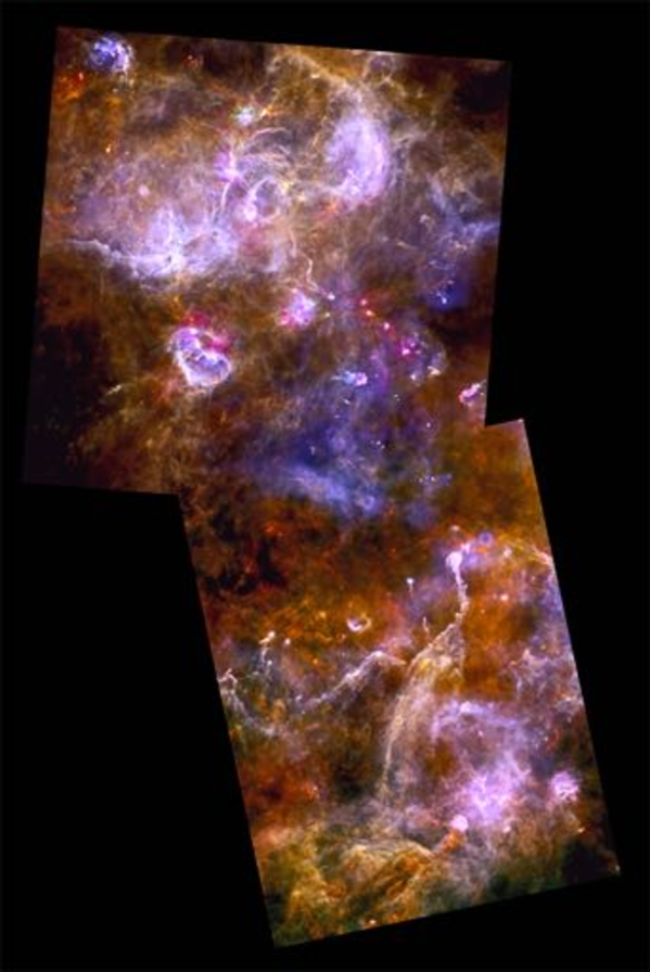
Figure 1: Three-colour image (blue=70 $\mu$m, green=160 $\mu$m, red=500 $\mu$m, all maps are absolutely calibrated) of the Cygnus X complex (credit: ESA/PACS/SPIRE) oriented in RA/Dec, i.e., north to the top, east to the left. The Cyg OB2 association is located slightly above the center of the figure. The image covers a range of RA(2000)$\sim$20^h30^m to 20^h45^m and Dec(2000)$\sim$38^∘ and 43^∘. Blue colours indicate gas heated by high-mass stars of the cluster and white colours indicate smaller H II  regions that locally heat the gas and create bubble-like features. Colder extended emission mainly arising from the molecular cloud is shown in red. Numerous pillars and globules, in particular in the southern part of Cygnus X, point towards Cyg OB2.

1 Introduction

In the environment of high-mass stars, a rich diversity of large and small dusty gas condensations are produced under the influence of ionizing radiation. These structures have mainly been detected through optical observations (see, e.g., Herbig herbig1974 (1974), Schneps et al. schneps1980 (1980), and White et al. white1997 (1997) for an overview). Column-like features were named ‘elephant-trunks’, and more isolated globule-shaped objects were named ‘teardrop’ or ‘cometary’ globules. In particular Hubble and Spitzer revealed manifold examples and the detailed structure of pillars in Galactic H II  regions, like the famous Pillars of Creation in M16 or the giant dust pillars in Carina. Pillars have a column shape, are attached to their native molecular cloud, and cover scales from $\sim$0.5 pc up to a few pc in length. Globules (on similar size scales) are isolated and have a characteristic head-tail structure. Low-mass star formation can take place in pillars (Hester et al. hester1996 (1996), White et al. white1999 (1999)), and globules (e.g., Sugitani et al. sugitani2002 (2002)), but there are only a few examples of high-mass stars in globules. Intermediate-mass early B-stars have been found in a globule in Cygnus (Schneider et al. 2012a , Djupvik et al., in prep.), which is part of this study.

On smaller size scales ($<$0.5 pc), there is a whole collection of different expressions for observed features: small globules (‘EGGs’, evaporating gaseous globules) are interpreted as fragments of a cloud (e.g., Smith et al. smith2003 (2003)) which possibly form stars (McCaughrean & Andersen mccaughran2002 (2002)), while proplyds (O’Dell et al. odell1993 (1993)) are evaporating circumstellar disks. After the discovery of proplyds in the Orion Nebula (e.g., Laques & Vidal laques1979 (1979)) they were searched for in the vicinity of other OB associations. Wright et al. (wright2012 (2012)) found proplyd-like objects in the immediate environment of the Cyg OB2 association but doubted that these are all disk-features. Another group of tiny ($<$0.05 pc) isolated condensations were detected by Gahm et al. (gahm2007 (2007)) in various Galactic H II  regions who named them globulettes.

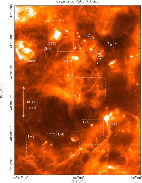
Figure 2: Herschel 70 $\mu$m PACS image (0 to 1000 MJy/sr) of the central region around Cyg OB2 (the most massive stars of the cluster are indicated by gray stars). The cross indicates the position of star Cyg OB2 #8 at RA(2000)=20^h33^m16^s and Dec(2000)=41^∘18^′45^′′, frequently used to define the center of Cyg OB2 (e.g., Wright et al. wright2015 (2015)). The H II  regions DR15, 18, 20, and 22 are labelled and the regions shown and discussed in more detail are outlined with dashed lines and numbered.

With Herschel far-infrared (FIR) imaging of high-mass star-forming regions within the HOBYS key program (Motte et al. motte2010 (2010)), it is now possible to detect these features in the FIR (provided that they are not too small) and also to determine systematically their physical properties such as size, mass, and temperature. At the same time, Herschel observations can provide a census of pre- and protostellar sources, and thus link the properties of pillars and globules to star formation within them. So far, Herschel observations have shown that the majority of low-mass stars form within filaments (e.g., André et al. andre2010 (2010), 2014), and OB clusters where filaments merge (e.g., Schneider et al. 2012b , Hennemann et al. hennemann2012 (2012)). It is not clear whether star formation in pillars, globules, proplyds etc. follows the same path. It is possible that dense filaments and accretion flows are shaped by UV radiation into the form of pillars, as was recently shown in numerical simulations with stellar feedback processes (Dale et al. dale2014 (2014)). These pillar-like features can then fragment into smaller units that evolve under the influence of radiation into globules, EGGs, condensations, proplyds, etc., depending on the intial pre-existing density structure, and finally form stars. The more classical view is that large-scale compression of an expanding H II region on a molecular cloud surface creates pillars that also evolve into globules, EGGs, condensations etc. Various studies (e.g., Lefloch & Lazareff lefloch1994 (1994), Williams et al. williams2001 (2001), Miao et al. miao2006 (2006), miao2009 (2009)) have shown that instabilities in the H II  region/molecular cloud interface create bright-rimmed clouds and pillars that can detach to form isolated globules. The importance of the turbulent gas structure was recognized by Gritschneder et al. (2009, 2010). Tremblin et al. (2012a,b) have shown that the turbulent density structure of molecular clouds can lead to local curvatures of the dense shell formed by the ionization compression, which may develop into pillars that can subsequently detach from the cloud. When the turbulent ram pressure of the molecular gas is larger than the ionized-gas pressure, globules can form.

In any case, both star-formation schemes outlined above produce isolated stars and the difference between them lies mainly in its primoridal phase. It is thus very difficult, perhaps impossible, to find observational which would allow us to discriminate between the two scenarios described.

Several HOBYS studies have already observed the H II  region/molecular cloud interface, including pillars, globules, and H II  bubbles, and how these are impacted by OB-clusters through heating (e.g., Schneider et al. schneider2010 (2010), Hill et al. hill2012 (2012), Anderson et al. anderson2012 (2012), and Didelon et al. didelon2015 (2015)), external compression (Zavagno et al. zavagno2010 (2010), Hill et al. hill2011 (2011), Minier et al. minier2013 (2013), Tremblin et al. tremblin2014 (2014)), and ionization (Deharveng et al. deharveng2012 (2012), Tremblin et al. tremblin2013 (2013)). In this paper, we focus on investigating the immediate environment of the Cyg OB2 association in the so-called Cygnus X region (see, e.g., Reipurth & Schneider reipurth2008 (2008) for an overview). Cygnus X is a large $\sim$10 degree wide radio emission feature (Piddington & Minnett piddington1952 (1952)) composed of numerous individual H II regions. A major problem is the uncertainty in distances because we look down a spiral arm, with the resulting confusion of regions as near as a few hundred parsec with others at 1-2 kpc and even well beyond. Kinematical distances in this region are very unreliable for distances up to $\sim$4 kpc because of the near-zero radial velocity gradient. For the objects studied in this paper, however, we do not expect a significant confusion because all spatially resolved objects clearly point towards Cyg OB2 and are thus shaped by the radiation of the stars.

Using the observational Herschel FIR-data (Sec. 2) and the Herschel derived column density, temperature, and FUV-field maps (Sec. 3 and 4), we classify the various features seen in the data (Sec. 5), calculate their lifetimes, and discuss their possible evolution (Sec. 6). A comparison of the pre- and protostellar sources found within various structures will be made in a subsequent paper.

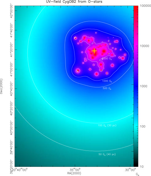
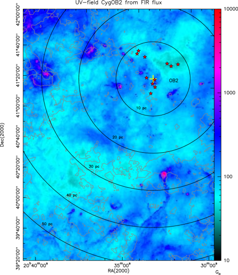
Figure 3: Left: UV-field in units of Habing (G₀) determined from a census of all O-stars given in Wright et al. (2015). Right: UV-field in units of Habing (G₀) for the central region around Cyg OB2 (limits as in Fig. 2) determined from the Herschel 70 $\mu$m and 160 $\mu$m fluxes. This image shows the impinging radiation. The most luminous O-stars of Cyg OB2 (Wright et al. 2015) are indicated as red stars and the yellow cross indicates the approximate center of the association. Concentric circles indicate the projected distance to this center in the plane of the sky, assuming a distance of 1.4 kpc to Cyg OB2. Gray contours (2 K kms^-1 to 22 K kms^-1 in steps of 2 K kms^-1) display line integrated (-10 to 20 km s^-1) ¹³CO 1$\to$0 emission at a resolution of 45^′′ (Schneider et al. schneider2011 (2011)).

2 Observations, dust column density and dust temperature maps

Two fields covering the Cygnus X region were observed with the Herschel satellite (Pilbratt et al. pilbratt2010 (2010)) in parallel mode. We present Herschel imaging observations at 70 $\mu$m and 160 $\mu$m from PACS (Photoconductor Array Camera and Spectrometer) (Poglitch et al. poglitsch2010 (2010)), and at 250 $\mu$m, 350 $\mu$m, and 500 $\mu$m from SPIRE (Spectral and Photometric Imaging Receiver) (Griffin et al. griffin2010 (2010)). Cygnus X South was observed on May 24, 2010 (obsIDs 1342196917 and 1342196918 for the nominal and orthogonal directions, respectively) and Cygnus X North on December 18, 2010 (obsIDs 13422211307 and 1342211308). This paper uses the observations of a part of both regions. The DR21 filament in Cygnus X North has already been presented in Hennemann et al. (hennemann2012 (2012), Herschel imaging) and White et al. (white2010 (2010), Herschel spectroscopy). For this paper, we employed a more recent HIPE (Herschel Interactice Processing Environment) version (10.0.2751) for the PACS and SPIRE data reduction in which we used modified pipeline scripts. Data collected during the turnaround of the satellite were included to insure a larger area was covered by the observations. The resulting Level1 contexts for each scan direction were combined using the ‘naive’ map maker in the destriper module. The conversion of the maps into surface brightness (from Jy/beam into MJy/sr) was made using the beam-areas obtained from measurements of Neptune (March 2013, see SPIRE handbook). The map offsets of the Level2 data were then determined using Planck and IRAS observations (Bernard et al. bernard2010 (2010)). The zero levels for the SPIRE 250 $\mu$m, 350 $\mu$m, and 500 $\mu$m data were also determined using the zeroPointCorrection task in HIPE and found to be consistent with offsets provided by J.-P. Bernard. PACS data were reduced up to Level1 using HIPE 10.0.2751 and then v. 20 of the Scanamorphos software package which performs baseline and drift removal before regridding (Roussel roussel2013 (2013)). See Hennemann et al. (hennemann2012 (2012)), Hill et al. (hill2011 (2011)) and Könyves et al. (vera2015 (2015)) for further details. The angular resolutions at 70 $\mu$m, 160 $\mu$m, 250 $\mu$m, 350 $\mu$m, and 500 $\mu$m, are $\sim$6^′′, $\sim$12^′′, $\sim$18^′′, $\sim$25^′′, and $\sim$36^′′, respectively.

Figure 1 shows a three-colour image of the whole Cygnus X region observed as part of the HOBYS program. The picture reveals impressively the way in which bright star-forming regions, emitting mainly at 70 $\mu$m and 160 $\mu$m (blue/green), are nestled in the larger cloud which is pervaded by a web of filaments. Colder gas is well traced by dust emission at 500 $\mu$m (red). At the very center, the diffuse blue emission of PACS at 70 $\mu$m indicates heating by the Cyg OB2 association (see Fig. 2 to locate the highest-mass stars). The H II  regions of Cygnus X (DR18, 20, and 22 in the northern region and DR15 in the southern region) stand out as bright emission regions in the three-colour image. The majority of pillars and globules in the figure, however, point towards the center of Cyg OB2, the most important source of UV-illumination (see Sec. 3). A zoom into the vicinity of Cyg OB2 is shown by a PACS image at 70 $\mu$m (Fig. 2); individual maps at 70 $\mu$m to 500 $\mu$m of these cutouts are shown in appendix A. In sections 5 and 6, we focus on the regions indicated in this plot and discuss the properties of the observed features.

Column density and dust temperature maps at an angular resolution of 36^′′ (all maps were smoothed to this lowest resolution of the 500 $\mu$m map) were made with a pixel-by-pixel SED fit from 160 $\mu$m to 500 $\mu$m, as described in, for example, Hill et al. (hill2011 (2011)). For the SED fit, we used a specific dust opacity per unit mass (dust and gas) approximated by the power law $\kappa_{\lambda}\,=\,0.1\,(\lambda/300\,{\rm\mu m})^{\beta}$ cm²g^-1 with $\beta$=2 (Roy et al. roy2014 (2014)), and left the dust temperature and column density as free parameters. We checked the SED fit of each pixel and determined from the fitted surface density the H₂ column density. The fit assumes a constant temperature for each pixel along the line of sight, an assumption that is not fullfilled in regions with strong temperature gradients. A detailed study of the dust properties in Orion A (Roy et al. roy2013 (2013)), however, showed that the single temperature model provides a reasonable fit, but that the dust opacity varies with column density by up to a factor of two. We thus estimate that the final uncertainties of the column density map are between 20% and 30%.

3 The FUV-field in Cygnus X

Cyg OB2 is one of the largest and most massive OB associations in the Galaxy with a mass of around 3$\times$10⁴ M_⊙ (Drew et al. drew2008 (2008)) at a distance of only 1.4 kpc (Rygl et al. rygl2012 (2012) from parallax observations). It is the richest aggregate in the Cygnus X region (e.g., Hanson hanson2003 (2003), Comerón & Pasquali comeron2012 (2012)), though the whole Cygnus X region contains several OB-associations, and is clearly the most important source of FUV-impact for the features we study here. A recent inventory of the central massive stars in Cyg OB2 compiles 52 O-stars and 3 Wolf-Rayet stars (Wright et al. wright2015 (2015)). They are the most important sources of feedback (radiation, winds) though the whole Cyg OB2 association is more extended (Comerón et al. comeron2008 (2008), Comerón & Pasquali comeron2012 (2012)). We evaluate the FUV-field expressed as a Habing field, produced by the 52 O-stars listed in Wright et al. (wright2015 (2015)). The ionising fluxes (Wright et al., priv. comm.) were calculated taking into account not just their spectral types, but also their exact luminosities, and binary companions. The most recent stellar atmosphere models were used, including the revised effective temperature scale in Martins et al. (martins2005 (2005)), and the luminosity shift that this leads to. We assume a simple 1/r² decrease of the flux and project all stars in the plane of the sky, ignoring possible attenuation by diffuse gas and blocking by molecular clumps. Additional sources of illumination, for example the more widespread O- and B-star population of Cyg OB2, are also not considered in this method. The resulting FUV-field is shown in Fig. 3 (left panel). Obviously, the field is strongest in the immediate environment of the stars, that is, the central 10 pc circle, reaching values of up to a few 10⁵ G₀ and drops to $\sim$50 G₀ in 40 pc distance.

In a second approach, we estimate the FUV-field from the total FIR intensity ($I_{FIR}$), assuming that the radiation from the massive stars heating the dust is re-radiated mainly at FIR wavelengths. With Herschel, we evaluate the FUV-field by adding the intensities at 70 $\mu$m and 160 $\mu$m (at an angular resolution of 12^′′) to I_FIR [10^-17 erg cm^-2 s^-1 sr^-1] (see Kramer et al. kramer2008 (2008), Roccatagliata et al. rocca2013 (2013) for the methodology):

$$F_{fuv}[G_{0}]\,\,=\,\,(4\,\pi I_{FIR}\,1000)/1.6$$ (1)

Note that the use of 160 $\mu$m emission as a tracer of the FUV-field can be disputable in regions dominated by cooler gas (which is not the case for Cygnus X) because flux at this wavelength can also come from cold thermal dust emission from the molecular cloud (the wavelength range 160 $\mu$m to 500 $\mu$m is used for the SED fit to determine the column density). For Cygnus X, the 160 $\mu$m emission contributed approximately 20% to the total UV-field, displayed in Fig. 3 (right), that ranges between a few hundred G₀ to more than 10⁴ G₀.

This method emphasizes the PDR surfaces that stand out prominently. These are illuminated by a UV-field of at least a few hundred G₀. Internal H II  regions can also contribute to the local FUV-field as in the case of the bright globule (g1) in Cygnus X (see below) that contains early B-stars. Here, the average UV-field across the globule head is 550 G₀ (see Table 1), but increases up to 7500 G₀ in a 12^′′ beam at the position of the B-star. Note, however, that the UV-field can only be calculated on the surfaces of molecular condensations (clumps, filaments, pillars, globules, etc.). In the ionized phase, the UV-field is, of course, present but can not be evaluated with this method. Instead, the field is estimated as outlined above, that is, from the photon flux of the stars (Fig. 3, right). The maps are thus not comparable but complementary, and a combination of both maps probably represents the overall FUV-field in Cygnus X best.

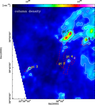
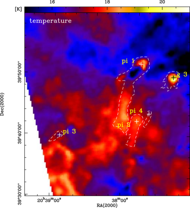
Figure 4: Region 1-1: column density (left) and dust temperature (right). Pillars are indicated by ‘pi’, globules by ‘g’, proplyds/proplyd-like by ‘pr’, condensations by ‘c’, and EGGs by ‘e’. The red dashed (white dashed in the right panel) contours outline the source shape based on the 70 $\mu$m map (derived from the 400 MJy/sr threshold). The column density contours correspond to the levels 1.5 and 2.0 10²² cm^-2.

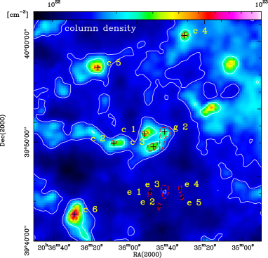
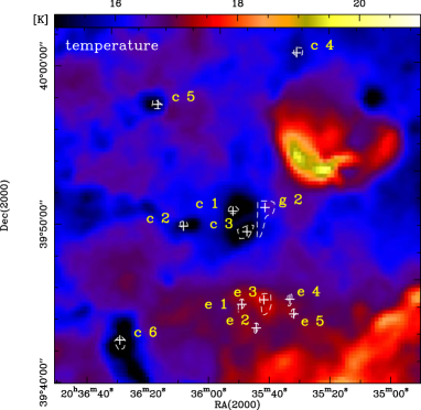
Figure 5: Region 1-2: as in Fig. 4. The column density contours correspond to the levels 1.5 and 2.3 10²² cm^-2.

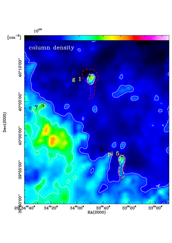
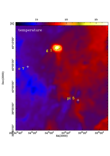
Figure 6: Region 1-3: as in Fig. 4. The column density contours correspond to the levels 1.5 and 2.3 10²² cm^-2.

4 Identification of objects

From the five Herschel wavelength bands, the 70 $\mu$m map (Fig. 2 and Appendix A) is the best suited to trace UV-illuminated features because the emission at 70 $\mu$m arises from warm dust and has the highest angular resolution (6^′′). The maps at shorter wavelengths (70 $\mu$m, 160 $\mu$m, and 250 $\mu$m) all start at 0 MJy/sr and show that with increasing wavelength, the amount of emission from colder dust increases and is visible as a diffuse background.

The 70 $\mu$m maps are dominated by emission from UV-heated dust, and so pillars, globules, and other features clearly stand out from a lower background, as is indicated by the contour at 400 MJy/sr (i.e., the sharp transition from red to green in the map). We thus used this contour to trace UV-illuminated features in the 70 $\mu$m maps and not the maps at longer wavelengths that are dominated by cold dust, mixed with mostly molecular gas. For display reasons, we set the lower limits to 150 MJy/sr and 70 MJy/sr for the 350 $\mu$m and 500 $\mu$m maps, respectively. The 500 $\mu$m maps thus show only the densest parts of the objects, that is, the heads of pillars or globules which are also traced in the column density maps. It is only with the temperature maps, that it is possible to distinguish whether the gas is warm or cold.

For display reasons, we divided the map shown in Fig. 2 into subregions covering many observed features. The resulting maps reveal many objects with different shapes and sizes in the vicinity of the Cyg OB2 cluster. As explained above, we take the contour level 400 MJy/sr (shown in the individual 70 $\mu$m maps of each subregion; see Appendix A) as a threshold to define the borders of all objects. This contour typically corresponds to a column density of 1–2$\sim$10²² cm^-2. We note, however, that the shape of the objects defined in the 70 $\mu$m maps do not always correspond one-to-one to the column density contour. For example, clumps within molecular clouds are prominent column density peaks but do not show up in the 70 $\mu$m map. We classified elongated, column-like structures that are still attached to the molecular cloud as pillars, isolated head-tail features as globules when they are large (typically $>$1^′) and prominent and as EGGs when they are small ($<$1^′) and faint. Centrally condensed objects without tails were called condensations. The term proplyd-like was used for the sources given in Wright et al. (wright2012 (2012)) as well as to some new ones, which probably fit into this scheme, detected in the Herschel images. All other features in the map that we did not classify have a more or less arbitrary shape and are most often bright edges of H II  regions. Our classification is complete, within the observed area, though we do not cover the whole Cygnus X region. Our main objective, however, is to derive typical values and discuss differences between the features representing different object classes in the various subregions.

The contours and labels of the objects identified in this way are shown in the column density and temperature maps of each subregion (see Figs. 4 to 10). Obviously, for some sources, the shape outlined by the 70 $\mu$m contour does not fully correspond to its shape in the column density or temperature map. For example, Pillar 1 in region 1-1 (Fig. 4) consists of a dense head with two peaks in column density of which one is cold ($\sim$14 K) and the other warm ($\sim$19 K), while the base of the pillar does not show up in the column density map. With this caveat in mind, we then determine the physical properties (column density, temperature, density, mass, length and width or radius, etc.) of the objects (Table 1 lists these quantities). In the following sections, we qualitatively describe the maps and objects and quantitatively discuss their various properties.

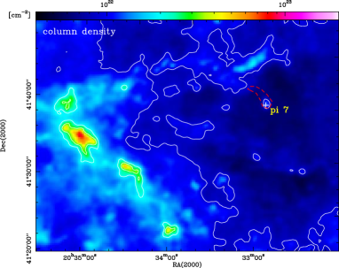
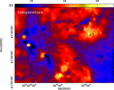
Figure 7: Region 3-2: as in Fig. 4. The column density contours correspond to the levels 1.0 and 1.7 10²² cm^-2.

Source	$\langle N(H_{2})\rangle$	$M$	$\langle n(H_{2})\rangle$	$\langle$T$\rangle$	Tmin	Tmax	$r$	$l\times w$	$\Sigma$	$\langle$flux$\rangle$
	[1021 cm-2]	[M⊙]	[103 cm-3]	[K]	[K]	[K]	[pc]	[pc$\times$pc]	[M⊙/pc2]	[Go]
	(1)	(2)	(3)	(4)	(5)	(6)	(7)	(8)	(9)	(10)
Pillars
1	21.0	1680	2.9	17.3	14.8	18.7	1.17	2.86 $\times$ 0.46	390	198
2	11.5	282	3.1	17.7	17.4	18.2	0.65	1.22 $\times$ 0.31	213	147
3	16.1	83	8.8	17.1	16.7	17.3	0.30	0.61 $\times$ 0.17	298	177
4	11.5	50	6.9	17.3	16.8	17.4	0.27	0.63 $\times$ 0.13	213	122
5	17.2	156	7.1	17.1	16.2	17.4	0.39	0.87 $\times$ 0.18	319	175
6	21.0	1403	3.2	18.0	17.3	20.2	1.07	2.38 $\times$ 0.43	390	295
7	7.9	86	3.0	19.1	18.1	20.1	0.43	0.88 $\times$ 0.24	147	191
mean	15.2$\pm$1.9	534$\pm$263	5.0$\pm$0.9	17.7$\pm$0.3	16.8$\pm$0.4	18.5$\pm$0.5	0.61$\pm$0.14		281$\pm$35	186$\pm$21
Globules
1	14.2	238	4.3	19.7	17.2	26.3	0.54		263	549
2	22.1	108	23.8	16.1	15.7	16.5	0.29		410	156
3	30.6	180	15.8	17.5	15.6	20.2	0.31		568	294
4	15.0	1356	2.0	19.7	18.6	23.7	1.24		279	428
mean	20.5$\pm$3.8	470$\pm$296	12$\pm$5	18.3$\pm$0.9	16.8$\pm$0.7	21.7$\pm$2.1	0.60$\pm$0.22		380$\pm$71	357$\pm$85
EGGs
1	12.9	10.8	18.6	17.1			0.11		239	137
2	11.7	5.9	22.8	17.0			0.08		217	113
3	13.5	38.6	10.1	17.3			0.22		251	153
4	13.5	4.5	34.4	16.9			0.06		251	137
5	12.8	6.4	25.0	17.1			0.08		238	127
mean	12.9$\pm$0.3	13$\pm$6	22$\pm$4	17.1$\pm$0.1			0.11$\pm$0.03		239$\pm$6	133$\pm$7
Proplyd-like
1	10.9	11.0	13.5	17.1			0.12	0.12 $\times$ 0.08	202	160
2	10.5	5.3	20.4	17.8			0.08	0.31 $\times$ 0.11	194	211
3	16.2	48.8	11.7	17.8			0.22	0.55 $\times$ 0.29	300	394
4	13.1	24.2	12.3	17.6			0.17	0.49 $\times$ 0.16	243	315
5	17.4	69.9	10.9	17.2			0.26	0.36 $\times$ 0.20	322	340
5a	13.8	37.0	10.6	17.2			0.21		256	192
5b	12.7	23.5	12.0	17.1			0.17		236	157
5c	12.7	17.0	14.1	17.0			0.15		235	171
5d	12.3	12.4	16.0	17.2			0.12		229	179
6	21.1	84.9	13.2	16.9			0.26	0.37 $\times$ 0.13	392	296
7	12.8	42.8	8.8	18.3			0.24	0.37 $\times$ 0.11	237	349
8	13.7	50.5	9.0	17.2			0.25	0.21 $\times$ 0.07	254	314
9	10.5	3.5	26.8	17.4			0.06	0.09 $\times$ 0.06	195	138
10	14.6	26.9	13.7	17.7			0.17	0.40 $\times$ 0.13	270	255
11	26.0	34.9	28.9	17.7			0.15		483	394
12	10.2	8.5	14.7	17.3			0.11		189	128
13	11.8	11.9	15.4	17.4			0.12		219	144
mean	14.1$\pm$1.0	31$\pm$6	15$\pm$1	17.4$\pm$0.09			0.17$\pm$0.02		262$\pm$19	243$\pm$23
Condensations
1	32.6	21.9	53.5	14.4			0.10		605	110
2	26.3	8.8	67.0	15.1			0.06		488	123
3	29.8	49.8	29.4	15.3			0.16		552	122
4	32.4	21.7	53.1	15.5			0.10		601	168
5	42.4	21.3	82.7	15.1			0.08		787	156
6	59.3	69.5	70.9	15.1			0.14		1100	272
7	25.0	30.0	30.0	15.3			0.14		465	131
mean	35.4$\pm$4.5	35$\pm$5	55$\pm$8	15.1$\pm$0.1			0.11$\pm$0.01		657$\pm$84	155$\pm$21

Table 1: Physical properties of pillars, globules, EGGS, proplyd-like, and condensations. The last line of each section gives the average (mean) values for each class of sources in bold.

5 Results

5.1 Description of maps

Regions 1-1, 1-2, and 1-3 (Figs. 4, 5, 6) contain five pillars and two globules and some examples of EGGs (five in total gathered in a ‘swarm’, named e1 to e5), best visible in the 70 $\mu$m Herschel map in the Appendix. They have the same orientation toward north as globule g2 suggesting that they are being influenced by Cyg OB2. The condensations (c1 to c3) in subregion 1-2 are also faint but are more spherical and show up mainly at 500 $\mu$m.

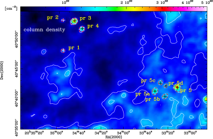
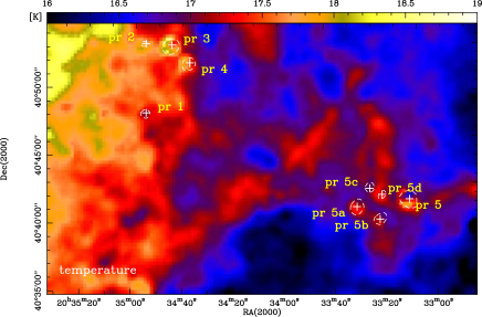
Figure 8: Region 2-1: as in Fig. 4. The column density contours correspond to the levels 1.0 and 1.2 10²² cm^-2.

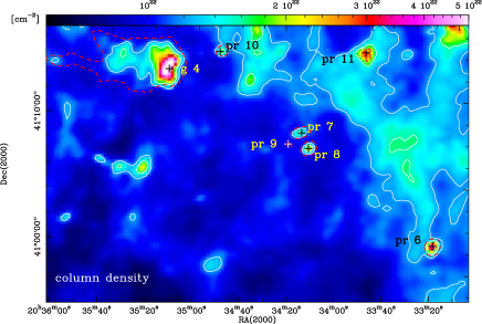
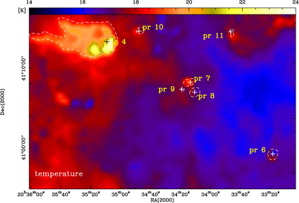
Figure 9: Region 2-2: as in Fig. 4. The column density contours correspond to the levels 1.2 and 1.6 10²² cm^-2.

Regions 2-1 and 2-2 (Figs. 7, 8) contain the ten Cyg OB2 proplyd-like objects reported by Wright et al. (wright2012 (2012)) that were detected in H$\alpha$ and Spitzer images. Two sources look spherical (pr1, pr8) in the Herschel images, even in the highest angular resolution 70 $\mu$m map, and can thus be partly unresolved, while the others have more complex head/tail shapes with bright ionization fronts that are oriented towards the center of Cyg OB2. However, all proplyd-like objects show an elongated structure pointing toward the center of Cyg OB2 in high resolution optical and near-IR images (Wright et al. wright2012 (2012)). Close to proplyd #5 (Wright et al. 2012), we detected some additional faint features that we name pr5a-d. The size scale of all these objects is typically around 0.1 pc, in agreement with what Wright et al. found. These authors are not certain about the nature of these features, suggesting that they are photo-evaporating protostars and naming them proplyd-like objects. Guarcello et al. (guarcello2013 (2013)) classified some of them as embedded stars with disks, and a recent spectroscopic study (Guarcello et al. guarcello2014 (2014)) showed that at least #5 and #7 are actively accreting protostars and that the disk of #7 is photoevaporating. Globule g4 coincides with the H II  region DR18, which hosts a strong IR-source (IRAS20343+4129, MSX6G080.3624+00.4213) at near-, mid-, and far-IR wavelengths. Comerón & Torra (comeron1999 (1999)) observed DR18 at IR and optical wavelengths and found an arc-shaped nebula, externally illuminated by a nearby B0.5V star. The globular shape is most likely caused by the object’s proximity to the Cyg OB2 cluster (see Fig. 2), though this source is not a typical example of a globule (like g1) because it is significantly more massive and extended.

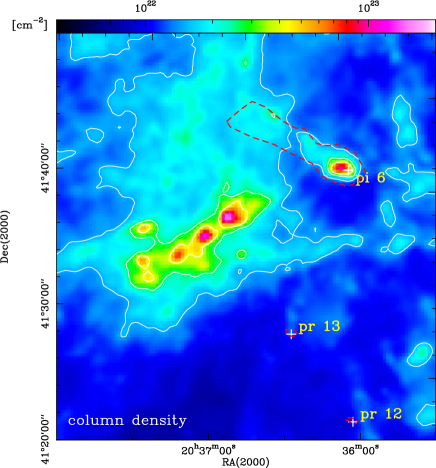
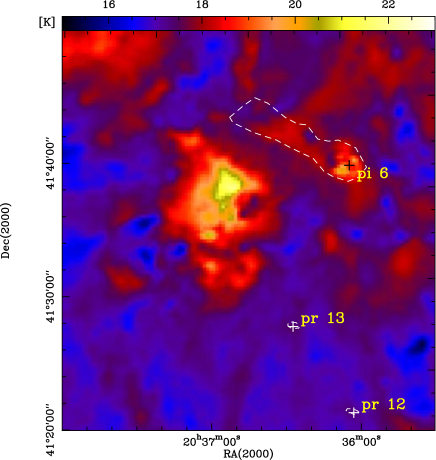
Figure 10: Region 3-1: as in Fig. 4. The column density contours correspond to the levels 1.5 and 4.0 10²² cm^-2.

Region 3-1 (Fig. 9) corresponds to the star-forming region DR20 (e.g., Odenwald et al. odenwald1990 (1990)) and includes one of the largest and most prominent pillars (pi6) in the Cyg OB2 environment. The pillar clearly points towards the center of OB2.
Region 3-2 (Fig. 10) contains another pillar (pi7) and three cold, irregularly shaped gas clumps. These clumps are probably not influenced by the close-by Cyg OB2 cluster because they have no preferred direction, in contrast to pi7 which points clearly towards the cluster center. Although projection effects can not be excluded, it is more likely that the clumps are massive structures still embedded in a more extended molecular cloud, and which are probably forming small clusters because we observe internal heating (see temperature map).

5.2 Physical properties

Table 1 gives an overview of the column density $N$(H₂), mass $M$, density $n$, temperature $T$, equivalent radius $r$, length $l$ and width $w$ for the elongated features, surface density $\Sigma$, and UV-flux F_fuv (derived from the Herschel data), we determined for each object from the Herschel observations. The length and width of the pillars were directly measured on the 70 $\mu$m map. The column density maps were used to calculate average column density, density, and mass within the areas defined by the 70 $\mu$m contour at 400 MJy/sr that we used to identify different features (see Sec. 4). Mass was determined following Eq. (2), using the column density $N$(H₂) in cm^-2, distance $d$ in parsec, and area $A$ in square degrees (see, e.g., Schneider et al. schneider1998 (1998))

$$M = 6.6\,\times\,10^{-24}\,N(H_{2})\,d^{2}\,A\,\,\,.$$ (2)

We estimate that the column density, mass, and density values are correct to within a factor of $\sim$2. The uncertainties mainly arise from the assumed dust opacity, and the possible variation in temperature along the line-of-sight not accounted for in the SED fitting. We consider the error on the distance to be low because the distance of Cyg OB2 has been very accurately determined through parallax (Rygl et al. rygl2012 (2012)). Since all objects we discuss here are directly affected by this cluster they must be at more or less the same distance. The minimum, maximum and average temperatures given in the Table were derived from the temperature maps. Since proplyd-like objects, EGGs, and condensations were barely resolved, minimum and maximum values were omitted. We did not include any irregular features in the Table because they do not form an individual class of objects, but are mostly H II  regions. The last line in each source category lists the average (mean) value. The main results extracted from the table are:

Size and density
EGGs, proplyd-like objects, and condensations are small (typically 0.1 pc to 0.25 pc). Their average densities are 2$\times$10⁴ cm^-3, 1.5$\times$10⁴ cm^-3, and 5.5$\times$10⁴ cm^-3, respectively. Comparing them to general molecular cloud features, condensations correspond to the dense cores typically found in submm-continuum imaging of high-mass star-forming regions (e.g., Motte et al. motte2007 (2007) for the Cygnus X region), but they are significantly larger and more massive than the dense cores found with Herschel in the nearby clouds of the Gould Belt (e.g., Könyves et al. vera2015 (2015)). The proplyd-like objects are much larger than the ones found in Orion A ($\sim$ a factor of 10, O’Dell et al. 1993), and also larger than those detected in the Carina nebula ($\sim$a factor of 2, Smith et al. smith2003 (2003)). Pillars and globules show a density gradient from high values $n>$10⁴ cm^-3 for the head, and $n<$10⁴ cm^-3 for the tail. The length of pillars varies between 0.6 pc and 3 pc.

Temperature
The temperature range of all objects is between 14 K and 26 K (average temperatures). The lowest temperatures are found for condensations ($\langle$T$\rangle\sim$ 15 K), and highest for globules ($\langle$T$\rangle\sim$18 K). All other objects typically have a temperature around 17 K. Pillars and globules show a temperature gradient from their warm UV-heated (external and possibly internal) head to a colder tail.

Mass
The highest mass objects (typically a few hundred M_⊙) are found amongst pillars and globules, mainly due to their large extents (e.g., equivalent radii larger than 0.5 pc) since their average densities ($\sim$5000 cm^-3) are low compared to the other features. We note, however, that the mass range can be quite varied, for example $\sim$50 M_⊙ for pi4 but $\sim$1700 M_⊙ for pi1. Their physical properties thus correspond to those typically derived for clumps inside molecular clouds (e.g., Schneider et al. schneider2006 (2006), Lo et al. lo2009 (2009)). Condensations and proplyd-like objects have masses of typically several tens of M_⊙ and EGGs have masses lower than 10 M_⊙. All objects are thus potential star-forming sites with large enough gas reservoirs to be so.

Surface density
Surface densities are highest for condensations and globules, i.e., $\sim$660 M_⊙/pc² and $\sim$380 M_⊙/pc², respectively. All other objects have $\langle\Sigma\rangle$ around 240–280 M_⊙/pc².

UV-flux
The UV-flux does not reflect an internal property of the detected features, it depends on its location and if it is only externally illuminated or contains an internal source. Obviously, high implied UV fluxes are found for all objects (mainly the proplyd-like objects), close to the central Cyg OB2 cluster. Two objects, globules g1 and g4, presumably have internal heating sources which explains their rather high implied average UV fluxes (549 G_∘ and 428 G_∘), respectively.

Source	$d_{OB}$	tphoto	texpos	ttotal	tff
	[pc]	[$10^{6}$ yr]	[$10^{6}$ yr]	[$10^{6}$ yr]	[$10^{6}$ yr]
	(1)	(2)	(3)	(4)	(5)
Pillars    $\langle n(H_{2})\rangle$=5$\times$103 cm-3, $\langle r\rangle$ = 0.61 pc
1	43.4	8.38	0.92	9.30	0.14
2	46.2	3.77	0.64	4.41	0.15
3	50.4	3.76	0.23	3.99	0.25
4	44.8	2.30	0.78	3.08	0.22
5	30.8	2.84	2.15	4.99	0.23
6	19.6	3.63	3.24	6.87	0.15
7	10.5	0.47	4.13	4.60	0.15
Globules    $\langle n(H_{2})\rangle$=12$\times$103 cm-3, $\langle r\rangle$ = 0.60 pc
1	26.6	2.35	2.56	4.91	0.16
2	36.4	5.10	1.60	6.70	0.41
3	42.0	6.19	1.05	7.24	0.34
4	11.5	1.66	4.03	5.69	0.12
Condensations    $\langle n(H_{2})\rangle$=55$\times$103 cm-3, $\langle r\rangle$ = 0.11 pc
1	37.8	3.58	1.46	5.04	0.62
2	37.8	2.54	1.46	4.00	0.69
3	37.8	4.00	1.46	5.46	0.46
4	32.2	3.02	2.01	5.03	0.62
5	33.8	3.92	1.86	5.78	0.77
6	39.7	7.71	1.28	8.99	0.71
7	29.4	2.44	2.29	4.73	0.46
EGGs    $\langle n(H_{2})\rangle$=22$\times$103 cm-3, $\langle r\rangle$ = 0.11 pc
1	37.8	1.48	1.47	2.95	0.37
2	38.1	1.22	1.44	2.66	0.40
3	38.6	2.04	1.39	3.43	0.27
4	37.1	1.28	1.54	2.82	0.50
5	37.8	1.32	1.47	2.79	0.42
Proplyd-like    $\langle n(H_{2})\rangle$=15$\times$103 cm-3, $\langle r\rangle$ = 0.17 pc
1	14.0	0.47	3.79	4.26	0.31
2	13.0	0.37	3.88	4.25	0.38
3	11.5	0.76	4.03	4.79	0.29
4	12.0	0.57	3.98	4.55	0.30
5	13.0	0.99	3.88	4.87	0.28
5a	13.2	0.72	3.86	4.58	0.28
5b	13.4	0.62	3.85	4.47	0.29
5c	13.0	0.56	3.88	4.44	0.32
5d	12.7	0.49	3.91	4.40	0.34
6	5.9	0.55	4.58	5.13	0.31
7	6.4	0.34	4.52	4.86	0.25
8	6.1	0.36	4.56	4.92	0.25
9	6.9	0.18	4.48	4.66	0.44
10	9.3	0.49	4.24	4.73	0.31
11	37.8	1.47	1.46	2.93	0.45
12	37.8	0.61	1.46	2.07	0.32
13	32.2	0.11	2.01	2.12	0.33

Table 2: Photoevaporation-, total-, and free-fall lifetimes of observed objects.

6 Analysis and discussion

The original ‘radiative driven implosion’ scenario (Bertoldi bertoldi1989 (1989), Lefloch & Lazareff lefloch1994 (1994), Miao et al. miao2009 (2009)) for the formation of pillars and globules involves UV-radiation illuminating a pre-existing clumpy molecular cloud and photoevaporating the lower density gas, leaving only the densest cores, which may collapse to form stars. Though recent hydrodynamic simulations including radiation (Gritschneder et al. gritschneder2009 (2009), 2010; Tremblin et al. 2012a , 2012b ) successfully model pillars and globules emphasizing the importance of turbulence, we will focus here on studying the lifetime of UV-illuminated features using the more classical approach.

6.1 Lifetimes

The model for photoevaporation of dense clumps we use here is based on that of Johnstone et al. johnstone1998 (1998). It calculates the mass loss rate $\dot{M}$ considering the external photon flux $\phi_{49}$, the number of ionizing photons from O-stars per second (in units of 10⁴⁹), that impinges on a clump with radius $r_{14}$ (in units of 10¹⁴ cm) at the distance to the central source $d_{17}$ (in units of 10¹⁷ cm):

$$\dot{M} = 9.5\times 10^{-9}\,\phi_{49}^{1/2}\,r_{14}^{3/2}\,d_{17}^{-1}\,\,[M_{\odot}/yr].$$ (3)

For the photon flux, we adopted as a lower limit the total flux from the most luminous O-stars clearly identified as members of Cyg OB2 in Hanson (hanson2003 (2003)) and Wright et al. (wright2015 (2015)), and ignored possible extinction. The total photon flux of 10^50.3 s^-1 was determined by their spectral type using the published values given in Sternberg et al. sternberg2003 (2003). Assuming a constant density but a variable radius, Eq. (3) can be solved analytically and we obtain for the time (t_photo) that it takes to completely photoevaporate the object

$$t_{photo} = 2.1\times 10^{20}\,\phi_{49}^{-1/2}\,(2\pi\,m_{H}/3)^{1/2}\,n_{3}^{1/2}\,d_{17}\,M^{1/2}\,\,[10^{6}yr],$$ (4)

with the number density $n_{3}$ in [10³ cm^-3] and the mass $M$ [M_⊙] from Table 1, and the mass of hydrogen $m_{H}$ [g]. In this simple approach, we neglected external compression which would increase t_photo because it reduces the size (i.e., radius) of the object which in turn lowers the mass loss rate. We note also that the values for the distances are only approximations because there is no clearly defined center of the Cyg OB2 association, and there are line-of-sight effects. The time of exposure to UV radiation for the object is estimated by t_expos = d_front/$v_{exp}$ km/s with the expansion velocity of $v_{exp}$ of the H II  region. In this paper we use a value of 10 km s^-1 for our calculations which is a typical value of expanding H II  regions (e.g., Williams et al. williams2001 (2001)).

This value is approximately in accord with that determined by comparing the relative velocity of the average radial stellar velocity of Cyg OB2 of -28 km s^-1 (Simbad data base) and the molecular cloud, that is –2 to -11 km s^-1 (Schneider et al. schneider2006 (2006)). Another way to approximate $v_{exp}$ is to use $v_{exp}\,=R_{b}/t_{OB2}$ with the extent of the bubble created by the H II  region $(R_{b}$ ), and the age of the Cyg OB2 association ($t_{OB2}$ ). The average radius of the bubble is $\sim$40 pc, derived from, for example, MSX-images (Schneider et al. schneider2006 (2006)) or the Canadian Galactic Plane Survey at 1.4 GHz (Reipurth & Schneider reipurth2008 (2008)). The cluster age is under discussion, with values ranging from 3–4 Myr (e.g., Comerón & Pasquali comeron2012 (2012)) and 5–7 Myr (e.g., Drew et al. drew2008 (2008), Wright et al. wright2015 (2015)). We thus determine an upper limit of $\sim$17 km s^-1 for $v_{exp}$ and a lower limit of $\sim$7 km s^-1. Considering the spread in values from the different methods, we take 10 km s^-1 as a conservative value and estimate that the lifetime calculations are correct within a factor of 1.5–2.

The photoevaportation lifetimes can be compared to the free-fall time for isothermal, gravitational collapse, as

$$t_{ff} = \sqrt{(}3/(2\,\pi\,G\,\rho),$$ (5)

in which $G$ is the gravitational constant and $\rho=n\,m_{H}$ the average volume density of the structure studied.

The calculated lifetime values are listed in Table 2. The most massive and extended objects – the pillars and globules – survive photoevaporation the longest, up to 8$\times$10⁶ yr. There is one exception, pi7, which has t_photo of only 5$\times$10⁵ yr. Condensations also have a relatively long photoevaporation lifetime ($\sim$2 to 8$\times$10⁶ yr). EGGs have shorter t_photo of 1–2$\times$10⁶ yr. For proplyd-like objects the photoevaporation lifetime is in the order of only a few 10⁵ yr. This timescale is consistent with what was estimated for the circumstellar disks in Orion (Johnstone et al. johnstone1998 (1998)) though it is not clear if all objects are indeed photoevaporating disks. The majority of the proplyd-like objects ($\sim$70%) actually already have stars within them, as evidenced by optical (Guarcello et al. guarcello2012 (2012)) and near-IR (Wright et al. wright2012 (2012)) point sources detected within them and the spectroscopy of two of their central stars (Guarcello et al. guarcello2014 (2014)), see also Sec. 5. Interestingly, Gahm et al. (gahm2007 (2007)) found lifetimes of about 4$\times$10⁶ yr for the globulettes in the Rosette Nebula, and IC1805, which have sizes smaller than 0.05 pc and average densities of 3–100$\times$10³ cm^-3. These longer photo evaporation times are likely due to much weaker FUV-field in these regions (both have far fewer O stars than Cyg OB2). Given our angular resolution, our census is not sensitive to these objects.

The ratio $t_{photo}/t_{expos}$ is an indicator of the evolutionary state of the structure. Pillars, globules, and condensations have an average ratio of $\sim$5, $\sim$2, and $\sim$3, respectively, suggesting that they are mostly in an early state of their evolution. EGGs typically have a ratio of one, which may imply that they are already half way through of being dissociated. Finally, proplyd-like objects have very small ratios of $\sim$0.05 and could be close to disappearing.

Taking objects’ current densities (Table 1), we estimate free-fall lifetimes typically of a few 10⁵ yr. Since $t_{ff}$ is proportional to $1/\sqrt{(}n)$, the densest objects - condensations - have the shortest collapse times, around 6$\times$10⁵ yr. The condensations, but also pillars, EGGs, and globules, are all potentially star-forming with $t_{ff}<t_{photo}$ and $t_{ff}\ll t_{total}$. Only proplyd-like objects have comparable lifetimes for photoevaporation and gravitational collapse. However, most of them, at least the original 10 from Wright et al. wright2012 (2012), have central stars observed in the optical or near-IR bands. We suspect that the large envelopes surrounding these stars will be eroded and destroyed within a short period of time which might influence how much more mass these stars can accrete, thus determining their final stellar masses.

6.2 An evolutionary sequence ?

Many detached structures (globules, proplyds, etc.) are observed in the Cygnus X region. The presence of such structures is also a signature found by Tremblin et al. (2012b ), when the initial turbulence in the molecular cloud dominates over the compression of the ionized gas. Hence, the turbulent pressure is likely to be as important in Cygnus X as the ionized gas pressure. Interestingly, Gritschneder et al. (gritschneder2009 (2009)) found dense pillar heads in their simulations and less material at the bases, which is a morphology seen for all pillars in Cygnus X. This behavior is also observed in the controlled simulations of Tremblin et al. (2012a , Fig. 5) and indicates that the structures are relatively old (see below), with pillars stretched until their heads are completely separated from the rest of the cloud.

The controlled runs in Tremblin et al. (2012a) represent a scenario of the interaction between an ionization front and a medium of constant density with a modulated interface geometry or a flat interface with density enhancements. They show that pillars with a large width/height ratio (w/h) will take a very long time (t) to grow. The narrowest pillar with an initial w/h= 0.5 (see Fig. 6 of Tremblin et al. (2012a) reached a length of 1.5 pc with w/h = 0.16 in 5$\times$10⁵ yr. In Cygnus X, the ratio R = w/h (Table 1) is on average 0.22, varying between 0.16 and 0.28, and the length of the pillars is between 0.6 pc and 3 pc with an average of 1.35 pc. If these values are compared to the ones shown in Tremblin et al. (2012a), see also Kinnear et al. (kinnear2014 (2014), kinnear2015 (2015)), the pillars observed in Cygnus X are likely to be quite well evolved. Only the curve with the smallest w/h ratio with large pillar sizes ($>$1 pc) is comparable to our observed values and hence indicates an evolutionary state of t$>$5$\times$10⁵ yr. This lower limit of t is consistent with the exposure time t_expos we calculated in Sec. 7.1 which ranges between 2$\times$10⁵ yr and 4$\times$10⁶ yr.

Putting together the physical properties determined from the Herschel observations (Sec. 5.2), the lifetime calculations (Sec. 6.1), and the results from comparison with simulations (see above), we propose a tentative evolutionary scheme for the observed features.

Pillars and globules are the most massive objects we see and they correspond in their physical properties (average size, density, and mass of $\sim$1 pc, 5–10 10³ cm^-3, and $\sim$500 M_⊙, respectively) to typical molecular cloud clumps. Condensations, and to a lesser extent EGGs, are likely molecular cloud dense cores with typical size and density of 0.1 pc and 2–6 10⁴ cm^-3, respectively. In this scheme, proplyd-like objects correspond to less dense (10³ cm^-3) cores. The main difference between these objects is that clumps and cores form as a part of a molecular cloud and are embedded in the clouds (e.g., cores within a filament), whereas globules, EGGs, condensations, and proplyd-like objects are isolated features. The resemblence of their physical properties, however, may suggest a filamentary origin as a possible scenario (see Introduction).

The remaining molecular envelopes of proplyd-like objects are less massive than those in the EGGs, probably because some of the mass has gone into the forming stars. Pillars form a special category because they are still attached to the cloud. This fact points towards a scenario in which pillars can be the eroded leftovers of a pre-existing clump or filament (Dale et al. dale2015 (2015)). Tremblin et al. (2012a,b) show that pillars can form either in a density- or surface-modulated region.

We find that pillars have the longest timescales for photoevaporation, mainly because they are massive and large, and have the smallest times of UV-exposure. We speculate that a pillar evolves into a globule and then on into a condensation. The major difference between globule and condensation is that the latter has no head-tail structure and is a factor of four denser and smaller. Larger globules might form multiple stars (see the example of globule g1 where several B-stars were found), possibly leading to multiple proplyd-like objects grouped together. This would also explain why the proplyd-like objects are grouped together a few at a time in little clumps. A condensation may be an evolved globule in which most of the lower density gas has photoevaporated away, leaving only a dense (5.5$\times$10⁴ cm^-3) and cold (T$\sim$15 K) core. We further speculate that EGGs and proplyd-like objects could be also leftovers of initially larger globules. As their name already indicates, EGGs, that is evaporating gaseous globules, have globular shapes. They are, however, less dense (2$\times$10⁴ cm^-3) and warm (T$\sim$17 K) and thus prone to disappear fast, in contrast to condensations that are potential sites of star/cluster formation. Proplyd-like objects may share the same fate as EGGs but they are on average more massive and extended and so likely to survive the photoevaporating impact of Cyg OB2 for longer. Given that some of them show signatures of star-formation activity, they could be the leftovers of condensations. If proplyd-like objects follow EGGs and if the latter have time to form stars, then it is not unreasonable to think that the former may have formed stars but still be surrounded by a portion of an envelope that is still finishing evaporating.

7 Summary

We used Herschel FIR imaging observations of the Cyg OB2 region, performed within the HOBYS keyprogram, to detect and characterize features that are formed in the interface region between H II  region and molecular cloud. Using a 400 MJy/sr flux threshold in the 70 $\mu$m map, we define pillars, globules, evaporating gaseous globules (EGGs), proplyd-like objects, and condensations. From SED fits to the 160–500 $\mu$m Herschel wavelengths, we determine column density and temperature maps, and derive masses, volume densities, and surface densities for these structures. From the 70 $\mu$m and 160 $\mu$m flux maps, we estimate an average FUV-field of typically a few hundred Habing on the photon dominated surfaces. We find that the initial morphological classification indeed corresponds to distinct objects with different physical properties.

$\bullet$ Pillars are the largest structures (equivalent mean average radius $\langle r\rangle\sim$0.6 pc). They have an average density of $\langle n\rangle\sim$5$\times$10³ cm^-3, and an average temperature $\langle T\rangle$ of 18 K. They often show temperature gradients along their longer axis. Their masses range between 50 M_⊙ and 1680 M_⊙, with an average mass $\langle M\rangle\sim$500 M_⊙.
$\bullet$ Globules are also large ($\langle r\rangle\sim$0.6 pc) but they have a more defined head-tail structure with a denser ‘head’ than pillars with $\langle n\rangle\sim$1.2$\times$10⁴ cm^-3. Their average mass and temperature are $\sim$500 M_⊙ and $\sim$18 K, respectively, similar to pillars.
$\bullet$ EGGs and proplyd-like objects are smaller ($r\sim$0.1 and 0.2 pc) and less massive ($\sim$10 M_⊙ and $\sim$30 M_⊙, respectively), but they have a high average density of 2.2$\times$10⁴ cm^-3 and 1.5$\times$10⁴ cm^-3, respectively. They both have an average temperature of 17 K.
$\bullet$ Condensations are small ($\sim$0.1 pc), have an average mass of 35 M_⊙, and are the densest structures we found in our sample with $\langle n\rangle\sim$5.5$\times$10⁴ cm^-3.

In summary, pillars and globules are irradiated structures which correspond to a subset of what is described as ‘clumps’ in molecular clouds while irradiated condensations correspond to a subset of massive dense molecular cloud ‘cores’. All pillars, globules and proplyd-like objects show a clear orientation toward the center of the Cyg OB2 association. They are thus directly influenced by the radiation of the stars and we used a census of them to estimate the lifetimes of all observed features using a model for photoevaporating dense clumps (Johnstone et al. johnstone1998 (1998)). Pillars and globules have the longest estimated photoevaporation lifetimes, a few million years, while all other features most likely survive less than a million years. These lifetimes are consistent with what was found in simulations of turbulent, UV-illuminated clouds (Tremblin et al. 2012a,b). We propose a tentative evolutionary scheme in which pillars can evolve into globules, which in turn then evolve into EGGs, condensations and proplyd-like objects.

Appendix A Herschel images at 70 to 500 $\mu$m of all regions

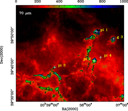
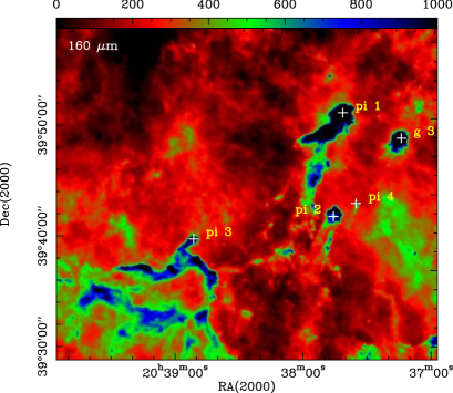
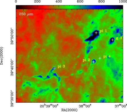
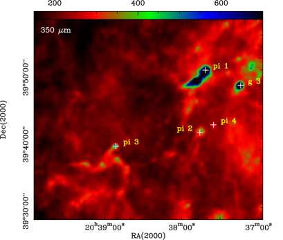
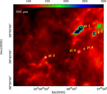
Figure 11: PACS (70 and 160 $\mu$m) and SPIRE (250, 350, 500 $\mu$m) images of region 1-1. All maps are in units of MJy/sr and the features classified as pillars (‘pi’), globules (‘g’), condensations (‘c’) and EGGS (‘e’) are indicated by yellow crosses in the plots. The black contour in the 70 $\mu$m map outlines the 400 MJy/sr level that was used to approximately define the shapes of the various features.

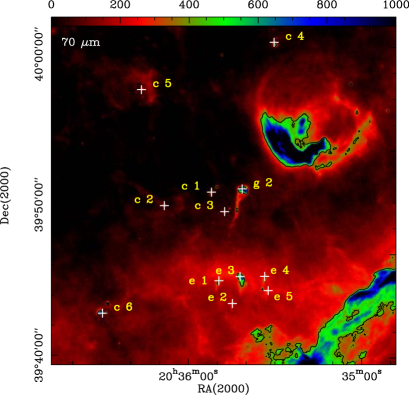
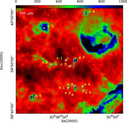
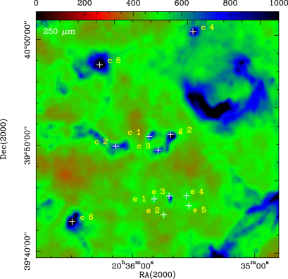
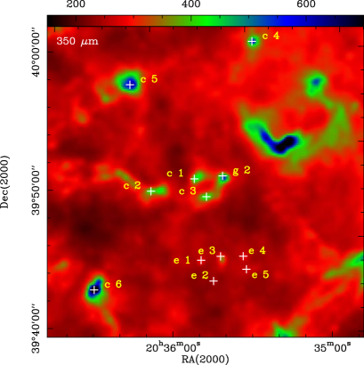
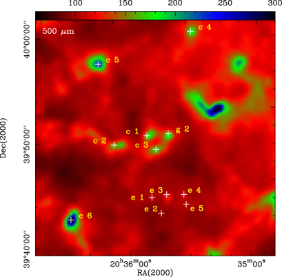
Figure 12: PACS (70 and 160 $\mu$m) and SPIRE (250, 350, 500 $\mu$m) images of region 1-2.

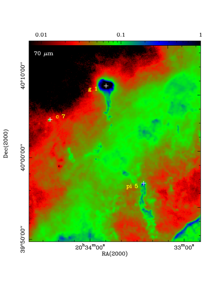
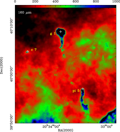
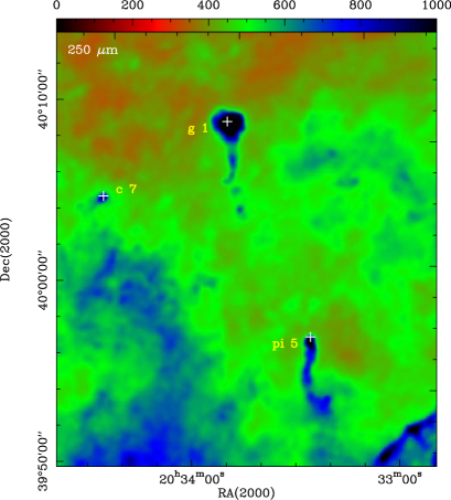
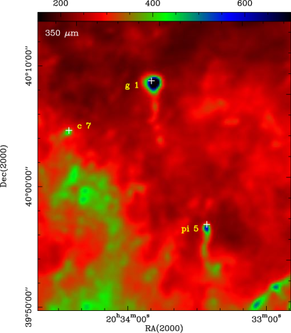
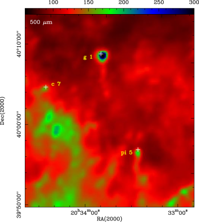
Figure 13: PACS (70 and 160 $\mu$m) and SPIRE (250, 350, 500 $\mu$m) images of region 1-3.

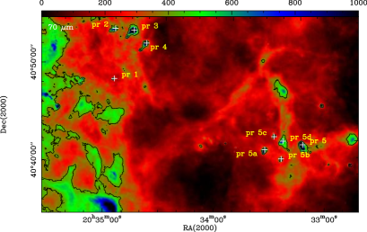
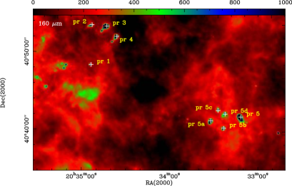
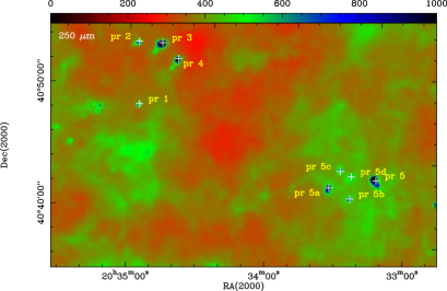
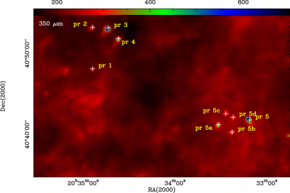
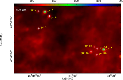
Figure 14: PACS (70 and 160 $\mu$m) and SPIRE (250, 350, 500 $\mu$m) images of region 2-1.

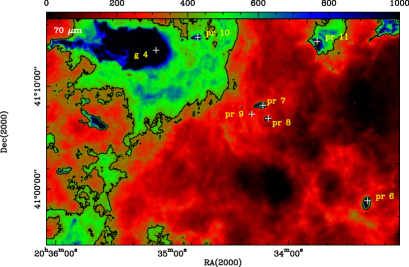
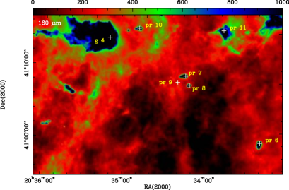
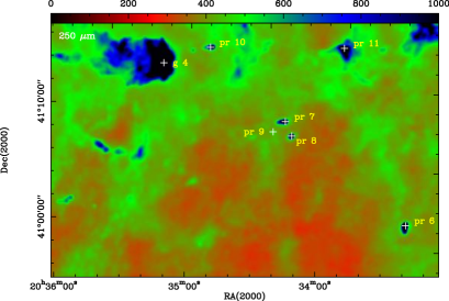
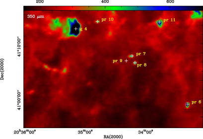
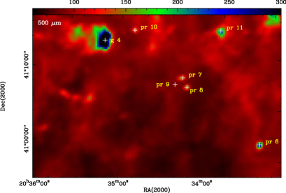
Figure 15: PACS (70 and 160 $\mu$m) and SPIRE (250, 350, 500 $\mu$m) images of region 2-2.

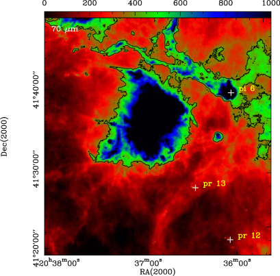
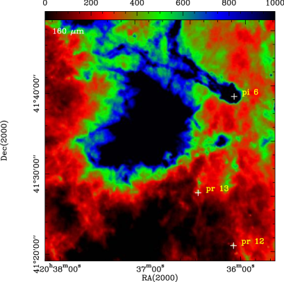
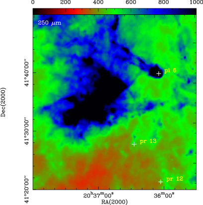
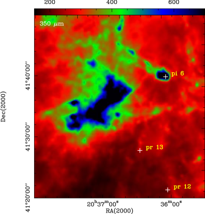
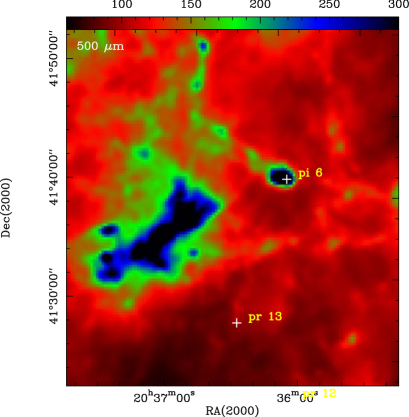
Figure 16: PACS (70 and 160 $\mu$m) and SPIRE (250, 350, 500 $\mu$m) images of region 3-1.

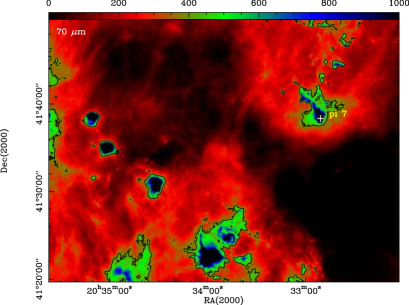
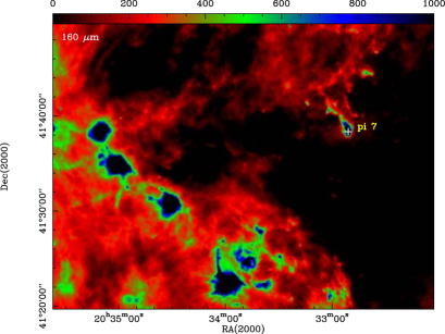
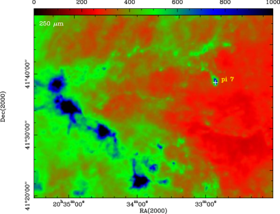
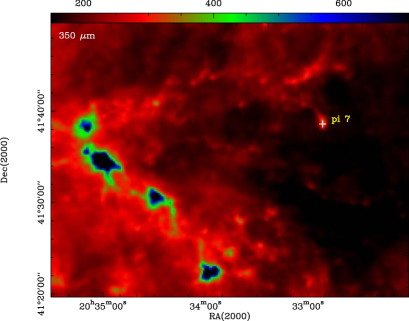
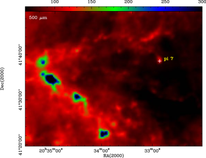
Figure 17: PACS (70 and 160 $\mu$m) and SPIRE (250, 350, 500 $\mu$m) images of region 3-2.