A traditional tree-style tableau for LTL:
LONG VERSION

Abstract

Propositional linear time temporal logic (LTL) is the standard temporal logic for computing applications and many reasoning techniques and tools have been developed for it. Tableaux for deciding satisfiability have existed since the 1980s. However, the tableaux for this logic do not look like traditional tree-shaped tableau systems and their processing is often quite complicated. We present a new simple traditional-style tree-shaped tableau for LTL and prove that it is sound and complete. As well as being simple to understand, to introduce to students and to use manually, it also seems simple to implement and promises to be competitive in its automation. It is particularly suitable for parallel implementations.

Note: the latest version of this report can be found via http://www.csse.uwa.edu.au/~mark/research/Online/ltlsattab.html.

1 Introduction

Propositional linear time temporal logic, LTL, is important for hardware and software verification[RV07]. LTL satisfiability checking (LTLSAT) is receiving renewed interest with advances computing power, several industry ready tools, some new theoretical techniques, studies of the relative merits of different approaches, implementation competitions, and benchmarking: [GKS10, SD11, RV07]. Common techniques include automata-based approaches [VW94, RV11] and resolution [LH10] as well as tableaux [Gou89, Wol85, KMMP93, Sch98b]. Each type of approach has its own advantages and disadvantages and each can be competitive at the industrial scale (albeit within the limits of what may be achieved with PSPACE complexity). The state of the art in tableau reasoners for LTL satisfiability testing is the technique from [Sch98b] which is used in portfolio reasoners such as [SD11].

Many LTL tableau approaches produce a very untraditional-looking graph, as opposed to a tree, and need the whole graph to be present before a second phase of discarding takes place. Within the stable of tableau-based approaches to LTLSAT, the system of [Sch98b] stands out in in being tree-shaped (not a more general graph), and in being one-pass, not relying on a two-phase building and pruning process. It also stands out in speed [GKS10]. However, there are still elements of communication between separate branches and a slightly complicated annotation of nodes with depth measures that needs to be managed as it feeds in to the tableau rules. So it is not in the traditional style of classical tableaux [BA12].

This paper presents a new simpler tableau for LTL. It builds on ideas from [SC85] and is influenced by LTL tableaux by [Wol85] and [Sch98b]. It also uses some ideas from a CTL* tableau approach in [Rey11] where uselessly long branches are curtailed. The general shape of the tableau and its construction rules are mostly unsurprising but the two novel PRUNE rules are perhaps a surprisingly simple way to curtail repetitive branch extension and may be applicable in other contexts.

The tableau search allows completely independent searching down separate branches and so lends itself to parallel computing. In fact this approach is “embarrassingly parallel” [Fos95]. Thus there is also potential for quantum implementations. Furthermore, only formula set labels need to be recorded down a branch, and checked back up the one branch, and so there is great potential for very fast implementations.

The soundness, completeness and termination of the tableau search is proved. The proofs are mostly straightforward. However, the completeness proof with the PRUNE rules has some interesting reasoning.

We provide a simple demonstration prototype reasoning tool to allow readers to explore the tableau search process. The tool is not optimised for speed in any way but we report on a small range of experiments on standard benchmarks which demonstrate that the new tableau will be competitive with the current state of the art [Sch98b].

In this paper we give some context in Section 2, before we briefly confirm our standard version of the well-known syntax and semantics for LTL in Section 3, describe our tableau approach is general terms section 4, present the rules section 5, make some comments and provide some motivation for our approach section 6, prove soundness in section 7, prove completeness in section 8, and briefly discuss complexity and implementation issues section 9, and detailed comparisons with the Schwendimann approach in Section 10, before a conclusion section 11.

The latest version of this long report can be found at http://www.csse.uwa.edu.au/~mark/research/Online/ltlsattab.html with links to a Java implementation of the tool and full details of experiments.

2 Context and Short Summary of Other Approaches

LTL is an important logic and there has been sustained development of techniques and tools for working with it over more than half a century. Many similar ideas appear as parts of different theoretical tools and it is hard for a researcher to be across all the threads. Thus it is worth putting the ideas here in some sort of context.

2.1 Satisfiability checking versus Model Checking

We will define structures and formulas more carefully in the next section but a structure is essentially a way of definitively and unambiguously describing an infinite sequence of states and an LTL formula may or may not apply to the sequence: the sequence may or may not be a model of the formula. See section 3 or [Pnu77] for details.

We are addressing a computational task called satisfiability checking. That is, given an LTL formula, decide whether or not there exists any structure at all which is a model of that formula. Input is the LTL formula, output is yes or no. The procedure or algorithm must terminate with the correct answer.

This problem is PSPACE complete in the size of formula [SC85].

There is a related but separate task called model checking. Model checking is the task of working out whether a given structure is a model or not of a given formula. Input is the LTL formula and a description of a system, output is yes or no, whether or not there is a behaviour generated by the system which is a model of the formula (or some variant on that). Model checking may seem to be more computationally demanding in that there is a formula and system to process. On the other hand, as described in [RV07] and outlined below, it is possible to use model checking algorithms to do satisfiability checking efficiently (in PSPACE). Model-checking itself, with a given formula on a given structure, is also PSPACE-complete [SC85], but in [LP85] we can find an algorithm that is exponential in the size of the formula and linear in the size of the model.

2.2 What is a tableau approach as compared to an automata-based approach or a reduction to model-checking

The thorough experimental comparison in [SD11] finds that across a wide range of carefully chosen benchmarks, none of the usual three approaches to LTL satisfiability testing dominates. Here we briefly introduce tableaux and distinguish the automata-based model-checking approach. Resolution is a very different technique and we refer the reader elsewhere, for example to [LH10, FDP01, HK03].

Tableau approaches trace their origins to the semantic tableaux, or truth trees, for classical logics as developed by Beth [Bet55] and Smullyan [Smu68]. The traditional tree style remains for many modal logics [Gir00] but, as we will outline below, this is not so for the LTL logic.

The tableau itself is (typically) a set of nodes, labelled by single formulas or sets of formulas, with a successor relation between nodes. The tree tableau has a root and the successor relation gives each node $0$, $1$ or $2$ children. The tableau is typically depicted with the root at the top and the children below their parent: thus giving an upside tree-shape.

Building a tableau constitutes a decision procedure for the logic when it is governed by rules for labelling children nodes, for counting a node as the leaf of a successful branch and for counting a node as the leaf of a failed branch. Finding one successful branch typically means that the original formula is satisfiable while finding all branches failing means it is not satisfiable. There are efficiently implemented tableau-based LTL satisfiability reasoning tools, which are easily available, such as pltl [Gor10] and LWB [LWB10]. We describe the approach and its variations in more detail in the next subsection.

The other main approach to LTL satisfiability checking is based on a reduction of the task to a model-checking question, which itself is often implemented via automata-based techniques. The traditional automata approach to model checking seen, for example in [VW94], is to compose the model with an automaton that recognizes the negation of the property of interest and check for emptiness of the composed structure.

Recently there has been some serious development of satisfiability checking on top of automata-based model-checking that ends up having some tableau-like aspects. The automata approach via model-checking as described in [RV07] shows that if you can do model checking you can do satisfiability checking. One can construct an automaton which will represent a universal system allowing all possible traces from the propositions. A given formula is satisfiable iff the universal system contains a model of the formula. By not actually building the universal system entirely the overall task can be accomplished in PSPACE in the size of formula. Some fast and effective approaches to satisfiability checking can then be developed by reasoning about the model checking using symbolic (bounded) SAT or BDD-based reasoners such as CadenceSMV and NuSMV [RV07]. Alternatively, explicit automata-based model-checkers such as SPIN [Hol97] could be used for the model checking but [RV07] shows these to not be competitive.

An important part of the symbolic approach is the construction of a symbolic automaton from the formula and this involves a tableau-like construction with sets of subformulas determining states. The symbolic automaton or tableau presented as part of the model-checking procedure in [CGH97] has been commonly used but this has been extended in [RV11] to a portfolio of translators. Also an LTL to tableau tool used in [RV11] is available via the first author’s website. We discuss these sorts of tableaux again briefly below.

The model-checking approach to LTL satisfiability checking is further developed in [LZP⁺13] where a novel, on-the-fly process combines the automata-construction and emptiness check. The tool out-performs previously existing tools for LTLSAT which use model-checking. Comprehensive experimental comparisons with approaches to LTLSAT beyond automata-theoretic model-checking based ones is left as future work.

2.3 Different shapes of tableaux and different ways to the search through the tableau

In some modal logics, and in temporal logics in particular, variations on the traditional tableau idea have been prevalent and the pure tree-shape is left behind as a more complicated graph of nodes is constructed. As we will see, this may happen in these variant tableaux, when the successor relation is allowed to have up-links from descendants to ancestors, cross-links from nodes to nodes on other branches, or where there is just an arbitrary directed graph of nodes.

Such a graph-shaped approach results if, for example, we give a declarative definition of a node and the successor relation determined by the labels on the node at each end. Typically, the node is identified with its label. Certain sets of formulas are allowed to exist as nodes and we have at most one node with a given label. Examples of this sort include the tableaux in [Gou84] and (the symbolic automaton of ) [CGH97].

Alternatively, the tableau may have a traditional form that is essentially tree-shped with a root and branches of nodes descending and branching out below that. Usually a limited form of up-link is allowed back from a node (leaf or otherwise) to one of its ancestors. There may be tableaux which contain several different nodes with the same label. Examples, include [Sch98a] and the new one. The new style tableau even allows multiple nodes down the same branch with the same labels while this is not permitted in [Sch98a].

The tableau construction may be incremental, where only reachable states are constructed, versus declarative, when we just define what labels are present in the tableau and which pairs of labels are joined by a directed edge.

A tableau is said to be one-pass if the construction process only build legitimate nodes as it proceeds. On the other hand, it is multi-pass if there is an initial construction phase followed by a culling phase in which some of the nodes (or labels) which were constructed are removed as not being legitimate.

A construction of a tableau, or a search through a tableau, will often proceed in a depth-first manner starting at a chosen node and then moving successively to successors. An alternative is via some sort of parallel implementation in which branches are explored concurrently. Search algorithms may make use of heuristics in guessing a good branch to proceed on. Undertaking a depth-first search in a graph-shaped label-determined tableau may seem to be similar to building a tree-shaped tableau but it is likely that the algorithm will behave differently when it visits a label that has been seen before down an earlier branch. In a tree-shaped tableau this may not need to be recorded.

Which is faster? Trees [Sch98a] may have 2EXPTIME worst case complexity. Graphs re-use labels and make many possible branches at one time: in general EXPTIME. However, [GKS10] demonstrated that the tree-shaped approach of [Sch98a] (consistently and sometimes drastically) outperformed the graph-shaped approach of [Wol85].

2.4 The Wolper and Schwendiman Tableau

Wolper’s [Wol83, Wol85] was the first LTL tableau. It is a multi-pass, graph-shaped tableau. The nodes are labelled with sets of formulas (from the closure set) with a minimal amount of extra notation attached to record which formulas already have been decomposed. One builds the graph starting at $\{\phi\}$ and using the standard sorts of decomposition rules and the transition rule. The tableau may start off looking like a tree but there must not be repeated labels so edges generally end up heading upwards and/or crossing branches. After the construction phase there is iterated elimination of nodes according to rules about successors and eventualities. (This approach was later extended to cover the inclusion of past-time operators in [LP00]).

There was a similar but slightly quicker proposal for a multi-pass, graph-shaped tableau for LTL in [Gou84]. The similar tableau in [KMMP93] is incremental but multi-pass as it builds a graph from initial states, then looks for strongly connected components (to satisfy eventualities). Other graph-like tableaux include those in [SGL97, MP95].

A graph-shaped tableau for LTL also forms part of the model-checking approach suggested in [CGH97]. Here the need to check fulfilment of eventualities is handed over to some CTL fairness constraint checking on a structure formed from the product of the tableau and the model to be checked. The symbolic model checker SMV is used to check the property subject to those fairness constraints. In [RV11], the ‘symbolic automaton’ approach based on the tableau from [CGH97] was adapted to tackle LTL satisfiability checking. Figure 1 shows a typical graph-style tableau from [CGH97].

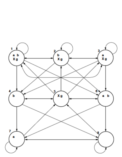
Figure 1: A graph-shaped tableau for $g=aUb$ from [CGH97]

Schwendimann’s tableau [Sch98a] is close to being purely tree-shaped (not a more general graph). It is also one-pass, not relying on a two-phase building and pruning process. However, there are still elements of communication between separate branches and a slightly complicated annotation of nodes with depth measures that needs to be managed as it feeds in to the tableau rules. In general, to decide on success or not for a tableau we need to work back up the tree towards the root, combining information from both branches if there are children. Thus, after some construction downwards, there is an iterative process moving from children to parents which may need to wait for both children to return their data. This can be done by tackling one branch at a time or in theory, in parallel. The data passed up consists in an index number and a set of formulas (unfulfilled eventualities). We describe this approach in more detail in Section 10. Figure 2 shows a typical tree-style tableau from [Sch98a].

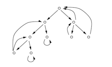
Figure 2: A tree-shaped tableau from [Sch98]

2.5 Implementations

The main available tools for LTL satisfiability checking are listed and described in [SD11]. These included pltl which (along with another tableau option) implements Schwendiammn’s approach.

We should also mention [LZP⁺13] here. The tool uses a novel, on-the-fly approach to LTLSAT via model-checking and out performs previously existing tools for LTLSAT which use the model-checking approach. There is an open source LTL to tableau translator available from Rozier’s website used for the [RV11] approach. Also, a more limited implementation was released open-source following the publication of [CGH97]: it is called ltl2smv and distributed with the NuSMV model checker.

2.6 Benchmarking

There is a brief comparison of the tableau approaches of Schwendimann and Wolper in [GKS10] and in [RV11] there is a comparison symbolic model-checking approaches.

However, the most thorough benchmarking exercise is as follows. Most known implemented tools for deciding satisfiability in LTL are compared in [SD11]. The best tools from three classes are chosen and compared: automata-based reduction to model-checking, tableau and resolution. A large range of benchmark patterns are collected or newly proposed. They find that no solver, no one of the three approaches, dominates the others. The tableau tool “pltl” based on Schwendimann’s approach is the best of the tableaux and the best overall on various classes of pattern. A portfolio solver is suggested and also evaluated.

The benchmark formulas, rendered in a selection of different formats, is available from Schuppan’s webpage.

2.7 So what is novel here?

The two PRUNE rules are novel. They force construction of branches to be terminated in certain circumstances. They depend only on the labels at the node and the labels of its ancestors. In general they may allow a label to be repeated some number of times before the termination condition is met.

The overall tableau shape is novel. Although tableaux are traditionally tree-shaped, no other tableau system for LTL builds graphs that are tree shaped. Most tableaux for LTL are more complicated graphs. The Schwendimann approach is close to being tree-shaped but there are still up-links from non-leaves.

The labels on the tableau are just sets of formulas from the closure set of the original formula (that is, subformulas and a few others). Other approaches (such as Schwendimann’s) require other annotations on nodes.

Overall tableau: one that is in completely traditional style (labels are sets of formulas), tree shaped tableau construction, no extraneous recording of calculated values, just looking at the labels.

Completely parallel development of branches. No communication between different branches. This promises interesting and useful parallel implementations.

The reasoning speed seems to be (capable of being) uniquely fast on some important benchmarks.

3 Syntax and Semantics

We assume a countable set $AP$ of propositional atoms, or atomic propositions.

A (transition) structure is a triple $(S,R,g)$ with $S$ a finite set of states, $R\subseteq S\times S$ a binary relation called the transition relation and labelling $g$ tells us which atoms are true at each state: for each $s\in S$, $g(s)\subseteq AP$. Furthermore, $R$ is assumed to be total: every state has at least one successor $\forall x\in S.\exists y\in S\mbox{ s.t.}(x,y)\in R$

Given a structure $(S,R,g)$ an $\omega$-sequence of states $\langle s_{0},s_{1},s_{2},...\rangle$ from $S$ is a fullpath (through $(S,R,g)$) iff for each $i$, $(s_{i},s_{i+1})\in R$. If $\sigma=\langle s_{0},s_{1},s_{2},...\rangle$ is a fullpath then we write $\sigma_{i}=s_{i}$, $\sigma_{\geq j}=\langle s_{j},s_{j+1},s_{j+2},...\rangle$ (also a fullpath).

The (well formed) formulas of LTL include the atoms and if $\alpha$ and $\beta$ are formulas then so are $\neg\alpha$, $\alpha\wedge\beta$, $X\alpha$, and $\alpha U\beta$.

We will also include some formulas built using other connectives that are often presented as abbreviations instead. However, before detailing them we present the semantic clauses.

Semantics defines truth of formulas on a fullpath through a structure. Write $M,\sigma\models\alpha$ iff the formula $\alpha$ is true of the fullpath $\sigma$ in the structure $M=(S,R,g)$ defined recursively by:
$M,\sigma\models p$ iff $p\in g(\sigma_{0})$, for $p\in{AP}$; $M,\sigma\models\neg\alpha$ iff $M,\sigma\not\models\alpha$; $M,\sigma\models\alpha\wedge\beta$ iff $M,\sigma\models\alpha$ and $M,\sigma\models\beta$; $M,\sigma\models X\alpha$ iff $M,\sigma_{\geq 1}\models\alpha$; and $M,\sigma\models\alpha U\beta$ iff there is some $i\geq 0$ s.t. $M,\sigma_{\geq i}\models\beta$ and for each $j$, if $0\leq j<i$ then $M,\sigma_{\geq j}\models\alpha$.

Standard Abbreviations in LTL include the classical $\top\equiv p\vee\neg p$, $\bot\equiv\neg\top$, $\alpha\vee\beta\equiv\neg(\neg\alpha\wedge\neg\beta)$, $\alpha\rightarrow\beta\equiv\neg\alpha\vee\beta$, $\alpha\leftrightarrow\beta\equiv(\alpha\rightarrow\beta)\wedge(\beta\rightarrow\alpha)$. We also have the temporal: $F\alpha\equiv(\top U\alpha)$, $G\alpha\equiv\neg F(\neg\alpha)$ read as eventually and always respectively. In reasoning with LTL, it is simpler to remove these abbreviations from input formulas and then deal with a relatively small set tableau rules for the disabbreviated language. However, experience with tableaux and typical real life LTL examples gives a strong indication that automated reasoning is quicker if these abbreviations are included as first-class language constructs in their own rights. Thus, inputs are accepted in the larger language including these symbols, they are not disabbreviated and there are enough tableau rules to process the bigger set of formulas directly. In this paper we present a tableau system with the larger set of rules.

A formula $\alpha$ is satisfiable iff there is some structure $(S,R,g)$ with some fullpath $\sigma$ through it such that $(S,R,g),\sigma\models\alpha$. A formula is valid iff for all structures $(S,R,g)$ for all fullpaths $\sigma$ through $(S,R,g)$ we have $(S,R,g),\sigma\models\alpha$. A formula is valid iff its negation is not satisfiable.

For example, $\top$, $p$, $Fp$, $p\wedge Xp\wedge F\neg p$, $Gp$ are each satisfiable. However, $\bot$, $p\wedge\neg p$, $Fp\wedge G\neg p$, $p\wedge G(p\rightarrow Xp)\wedge F\neg p$ are each not satisfiable.

We will fix a particular formula, $\phi$ say, and describe how a tableau for $\phi$ is built and how that decides the satisfiability or otherwise, of $\phi$. We will use other formula names such as $\alpha$, $\beta$, e.t.c., to indicate arbitrary formulas which are used in labels in the tableau for $\phi$.

4 General Idea of the Tableau

The tableau for $\phi$ is a tree of nodes (going down the page from a root) each labelled by a set of formulas. To lighten the notation, when we present a tableau in a diagram we will omit the braces $\{\}$ around the sets which form labels. The root is labelled $\{\phi\}$.

Each node has 0, 1 or 2 children. A node is called a leaf if it has 0 children. A leaf may be crossed ($\times$), indicating a failed branch, or ticked ($\surd$), indicating a successful branch. Otherwise, a leaf indicates an unfinished branch and unfinished tableau.

The whole tableau is successful if there is a ticked branch. This indicates a “yes” answer to the satisfiability of $\phi$. It is failed if all branches are crossed: indicating “no”. Otherwise it is unfinished. Note that you can stop the algorithm, and report success if you tick a branch even if other branches have not reached a tick or cross yet.

A small set of tableau rules (see below) determine whether a node has one or two children or whether to cross or tick it. This depends on the label of the parent, and also, for some rules, on labels on ancestor nodes, higher up the branch towards the root. The rule also determines the labels on the children.

The parent-child relation is indicated by a vertical arrow in diagrams (if needed). However, to indicate use of one particular rule (coming up below) called the TRANSITION rule we will use a vertical arrow ($\downarrow=$) with two strikes across it, or just an equals sign.

A node label may be the empty set, although it then can be immediately ticked by rule EMPTY below.

A formula which is an atomic proposition, a negated atomic proposition or of the form $X\alpha$ or $\neg X\alpha$ is called elementary. If a node label is non-empty and there are no direct contradictions, that is no $\alpha$ and $\neg\alpha$ amongst the formulas in the label, and every formula it contains is elementary then we call the label (or the node) poised.

Most of the rules consume formulas. That is, the parent may have a label $\Gamma=\Delta\mathbin{\mathaccent 0{\cdot}\cup}\{\alpha\}$, where $\mathbin{\mathaccent 0{\cdot}\cup}$ is disjoint union, and a child may have a label $\Delta\cup\{\gamma\}$ so that $\alpha$ has been removed, or consumed.

See the $\neg p\wedge X\neg p\wedge(qUp)$ example given in Figure 3 of a simple but succesful tableau.

Figure 3: $\neg p\wedge X\neg p\wedge(qUp)$

As usual a tableau node $x$ is an ancestor of a node $y$ precisely when $x=y$ or $x$ is a parent of $y$ or a parent of a parent, etc. Then $y$ is a descendent of $x$ and we write $x\leq y$. Node $x$ is a proper ancestor of $y$, written $x<y$, iff it is an ancestor and $x\neq y$. Similarly proper descendent. When we say that a node $y$ is between node $x$ and its descendent $z$, $x\leq y\leq z$, then we mean that $x$ is an ancestor of $y$ and $y$ is an ancestor of $z$.

A formula of the form $X(\alpha U\beta)$ or $XF\beta$ appearing in a poised label of a node $m$, say, also plays an important role. We will call such a formula an $X$-eventuality because $\alpha U\beta$ or $F\beta$ is often called an eventuality, and its truth depends on $\beta$ being eventually true in the future (if not present). If the formula $\beta$ appears in the label of a proper descendent node $n$ of $m$ then we say that the $X$-eventuality at $m$ has been fulfilled by $n$ by $\beta$ being satisfied there.

5 Rules:

There are twenty-five rules altogether. We would only need ten for the minimal LTL-language, but recall that we are treating the usual abbreviations as first-class symbols, so they each need a pair of rules.

Most of the rules are what we call static rules. They tell us about formulas that may be true at a single state in a model. They determine the number, $0$, $1$ or $2$, of child nodes and the labels on those nodes from the label on the current parent node without reference to any other labels. These rules are unsurprising to anyone familiar with any of the previous LTL tableau approaches.

To save repetition of wording we use an abbreviated notation for presenting each rule: the rule $A/B$ relates the parent label $A$ to the child labels $B$. The parent label is a set of formulas. The child labels are given as either a $\surd$ representing the leaf of a successful branch, a $\times$ representing the leaf of a failed branch, a single set being the label on the single child or a pair of sets separated by a vertical bar $|$ being the respective labels on a pair of child nodes.

Thus, for example, the $U$-rule, means that if node is labelled $\{\alpha U\beta\}\mathbin{\mathaccent 0{\cdot}\cup}\Delta$, if we choose to use the $U$-rule and if we choose to decompose $\alpha U\beta$ using the rule then the node will have two children labelled $\Delta\cup\{\beta\}$ and $\Delta\cup\{\alpha,X(\alpha U\beta)\}$ respectively.

Often, several different rules may be applicable to a node with a certain label. If another applicable rule is chosen, or another formula is chosen to be decomposed by the same rule, then the child labels may be different. We discuss this non-determinism later.

These are the positive static rules:
EMPTY-rule: $\{\}\;/\;\surd$. $\top$-rule: $\{\top\}\mathbin{\mathaccent 0{\cdot}\cup}\Delta\;/\;\Delta$. $\bot$-rule: $\{\bot\}\mathbin{\mathaccent 0{\cdot}\cup}\Delta\;/\;\times$. $\wedge$-rule: $\{\alpha\wedge\beta\}\mathbin{\mathaccent 0{\cdot}\cup}\Delta\;/\;(\Delta\cup\{\alpha,\beta\})$. $\vee$-rule: $\{\alpha\vee\beta\}\mathbin{\mathaccent 0{\cdot}\cup}\Delta\;/\;(\Delta\cup\{\alpha\}\;|\;\Delta\cup\{\beta\})$. $\rightarrow$-rule: $\{\alpha\rightarrow\beta\}\mathbin{\mathaccent 0{\cdot}\cup}\Delta\;/\;(\Delta\cup\{\neg\alpha\}\;|\;\Delta\cup\{\beta\})$. $\leftrightarrow$-rule: $\{\alpha\leftrightarrow\beta\}\mathbin{\mathaccent 0{\cdot}\cup}\Delta\;/\;((\Delta\cup\{\alpha,\beta\}\;|\;\Delta\cup\{\neg\alpha,\neg\beta\}))$. $U$-rule: $\{\alpha U\beta\}\mathbin{\mathaccent 0{\cdot}\cup}\Delta\;/\;(\Delta\cup\{\beta\}\;|\;\Delta\cup\{\alpha,X(\alpha U\beta)\})$. $F$-rule: $\{F\alpha\}\mathbin{\mathaccent 0{\cdot}\cup}\Delta\;/\;(\Delta\cup\{\alpha\}\;|\;\Delta\cup\{XF\alpha\})$. $G$-rule: $\{G\alpha\}\mathbin{\mathaccent 0{\cdot}\cup}\Delta\;/\;\Delta\cup\{\alpha,XG\alpha\}$.

There are also static rules for negations:
CONTRADICTION-rule: $\{\alpha,\neg\alpha\}\mathbin{\mathaccent 0{\cdot}\cup}\Delta\;/\;\times$. $\neg\neg$-rule: $\{\neg\neg\alpha\}\mathbin{\mathaccent 0{\cdot}\cup}\Delta\;/\;\Delta\cup\{\alpha\}$. $\neg\bot$-rule: $\{\neg\bot\}\mathbin{\mathaccent 0{\cdot}\cup}\Delta\;/\;\Delta$. $\neg\top$-rule: $\{\neg\top\}\mathbin{\mathaccent 0{\cdot}\cup}\Delta\;/\;\times$. $\neg\wedge$-rule: $\{\neg(\alpha\wedge\beta)\}\mathbin{\mathaccent 0{\cdot}\cup}\Delta\;/\;(\Delta\cup\{\neg\alpha\}\;|\;\Delta\cup\{\neg\beta\})$. $\neg\vee$-rule: $\{\neg(\alpha\vee\beta)\}\mathbin{\mathaccent 0{\cdot}\cup}\Delta\;/\;(\Delta\cup\{\neg\alpha,\neg\beta\})$. $\neg\rightarrow$-rule: $\{\neg(\alpha\rightarrow\beta)\}\mathbin{\mathaccent 0{\cdot}\cup}\Delta\;/\;(\Delta\cup\{\alpha,\neg\beta\})$. $\neg\leftrightarrow$-rule: $\{\neg(\alpha\leftrightarrow\beta)\}\mathbin{\mathaccent 0{\cdot}\cup}\Delta\;/\;((\Delta\cup\{\alpha,\neg\beta\}\;|\;\Delta\cup\{\neg\alpha,\beta\}))$. $\neg U$-rule: $\{\neg(\alpha U\beta)\}\mathbin{\mathaccent 0{\cdot}\cup}\Delta\;/\;(\Delta\cup\{\neg\alpha,\neg\beta\}\;|\;\Delta\cup\{\neg\beta,X\neg(\alpha U\beta)\})$. $\neg G$-rule: $\{\neg G\alpha\}\mathbin{\mathaccent 0{\cdot}\cup}\Delta\;/\;(\Delta\cup\{\neg\alpha\}\;|\;\Delta\cup\{X\neg G\alpha\})$. $\neg F$-rule: $\{\neg F\alpha\}\mathbin{\mathaccent 0{\cdot}\cup}\Delta\;/\;\Delta\cup\{\neg\alpha,X\neg F\alpha\}$.

The remaining four non-static rules are only applicable when a label is poised (which implies that none of the static rules will be applicable to it). In presenting them we use the convention that a node $u$ has label $\Gamma_{u}$. The rules are to be considered in the following order.

[LOOP]: If a node $v$ with poised label $\Gamma_{v}$ has a proper ancestor (i.e. not itself) $u$ with poised label $\Gamma_{u}$ such that $\Gamma_{u}\supseteq\Gamma_{v}$, and for each $X$-eventuality $X(\alpha U\beta)$ or $XF\beta$ in $\Gamma_{u}$ we have a node $w$ such that $u<w\leq v$ and $\beta\in\Gamma_{w}$ then $v$ can be a ticked leaf.

[PRUNE]: Suppose that $u<v<w$ and each of $u$, $v$ and $w$ have the same poised label $\Gamma$. Suppose also that for each $X$-eventuality $X(\alpha U\beta)$ or $XF\beta$ in $\Gamma$, if there is $x$ with $\beta\in\Gamma_{x}$ and $v<x\leq w$ then there is $y$ such that $\beta\in\Gamma_{y}$ and $u<y\leq v$. Then $w$ can be a crossed leaf.

[PRUNE₀]: Suppose that $u<v$ share the same poised label $\Gamma$. Suppose also that $\Gamma$ contains at least one $X$-eventuality but there is no $X$-eventuality $X(\alpha U\beta)$ or $XF\beta$ in $\Gamma$, with a node $x$ such that is $\beta\in\Gamma_{x}$ and $u<x\leq v$. Then $v$ can be a crossed leaf.

[TRANSITION]: If none of the other rules above do apply to it then a node labelled by poised $\Gamma$ say, can have one child whose label is: $\Delta=\{\alpha|X\alpha\in\Gamma\}\cup\{\neg\alpha|\neg X\alpha\in\Gamma\}$.

6 Comments and Motivation

A traditional classical logic style tableau starts with the formula in question and breaks it down into simpler formulas as we move down the page. The simpler formulas being satisfied should ensure that the more complicated parent label is satisfied. Alternatives are presented as branches. See the example given in Figure 4.

Figure 4: Classical disjunction

Figure 5: Until also gives us choices

We follow this style of tableau as is evident by the classical look of the tableau rules involving classical connectives. The $U$ and $\neg U$ rules are also in this vein, noting that temporal formulas such as $U$ also gives us choices: Figure 5.

Eventually, we break down a formula into elementary ones. The atoms and their negations can be satisfied immediately provided there are no contradictions, but to reason about the $X$ formulas we need to move forwards in time. How do we do this? See Figure 6.

Figure 6: But what to do when we want to move forwards in time?

Figure 7: Introduce a new type of TRANSITION

The answer is that we introduce a new type of TRANSITION step: see Figure 7. Reasoning switches to the next time point and we carry over only information nested below $X$ and $\neg X$.

With just these rules we can now do the whole $\neg p\wedge X\neg p\wedge(qUp)$ example. See Figure 3.

This example is rather simple, though, and we need additional rules to deal with infinite behaviour. Consider the example $Gp$ which, in the absence of additional rules, gives rise to a very repetitive infinite tableau. Figure 8.

Figure 8: $Gp$ gives rise to a very repetitive infinite tableau without the LOOP rule, but succeeds quickly with it

Figure 9: $G(p\wedge q)\wedge F\neg p$ crossed by PRUNE

Notice that the infinite fullpath that it suggests is a model for $Gp$ as would be a fullpath just consisting of the one state with a self-loop (a transition from itself to itself).

This suggests that we should allow the tableau branch construction to halt if a state is repeated. However the example $G(p\wedge q)\wedge F\neg p$ shows that we can not just accept infinite loops as demonstrating satisfiability: the tableau for this unsatisfiable formula would have an infinite branch if we did not use the PRUNE rule to cross it (Figure 9). Note that the more specialised PRUNE₀ rule can be used to cross the branch one TRANSITION earlier.

Notice that the infinite fullpath that the tableau suggests is this time not a model for $G(p\wedge q)\wedge F\neg p$. Constant repeating of $p,q$ being made true does not satisfy the conjunct $F\neg p$. We have postponed the eventuality forever and this is not acceptable.

If $\alpha U\beta$ appears in the tableau label of a node $u$ then we want $\beta$ to appear in the label of some later (or equal node) $v$. In that case we say that the eventuality is satisfied by $v$.

Eventualities are eventually satisfied in any (actual) model of a formula: by the semantics of $U$.

Thus we introduce the LOOP rule with an extra condition. If a label is repeated along a branch and all eventualities are satisfied in between then we can build a model by looping states. In fact, the ancestor can have a superset and it will work (see the soundness proof below).

Examples like $G(p\wedge q)\wedge F\neg p$ (in Figure 9) and $p\wedge G(p\rightarrow Xp)\wedge F\neg p$ which have branches that go on forever without satisfying eventualities, still present a problem for us. We need to stop and fail branches so that we can answer “no” correctly and terminate and so that we do not get distracted when another branch may be successful. In fact, no infinite branches should be allowed.

The final rule that we consider, and the most novel, is based on observing that these infinite branches are just getting repetitive without making a model. The repetition is clear because there are only a finite set of formulas which can ever appear in labels for a given initial formula $\phi$. The closure set for a formula $\phi$ is as follows:

$$\{\psi,\neg\psi|\psi\leq\phi\}\cup\{X(\alpha U\beta),\neg X(\alpha U\beta)|\alpha U\beta\leq\phi\}$$

Here we use $\psi\leq\phi$ to mean that $\psi$ is a subformula of $\phi$. The size of closure set is $\leq 4n$ where $n$ is the length of the initial formula. Only formulas from this finite set will appear in labels. So there are only $\leq 2^{4n}$ possible labels.

A similar observation in the case of the branching time temporal logic CTL* suggested the idea of useless intervals on branches in the tableau in [Rey11]. It is also related to the proof of the small model theorem for LTL in [SC85].

The PRUNE rule is as follows. If a node at the end of a branch (of a partially complete tableau) has a label which has appeared already twice above, and between the second and third appearance there are no new eventualities satisfied then that whole interval of states has been useless. The PRUNE₀ rule applies similar reasoning to an initial repeat in which no eventualities are fulfilled.

It should be mentioned that the tableau building process we describe above is non-deterministic in several respects and so really not a proper description of an algorithm. However, we will see in the correctness proof below that the further details of which formula to consider at each step in building the tableau are unimportant.

Finally a suggestion for a nice example to try. Try $p\wedge G(p\leftrightarrow X\neg p)\wedge G(q\rightarrow\neg p)\wedge G(r\rightarrow\neg p)\wedge G(q\rightarrow\neg r)\wedge GFq\wedge GFr$.

7 Proof of Correctness: Soundness:

Justification will consist of three parts: each established whether or not the optional rules are used.

Proof of soundness. If a formula has a successful tableau then it has a model.

Proof of completeness: If a formula has a model then building a tableau will be successful.

Proof of termination. Show that the tableau building algorithm will always terminate.

First, a sketch of the Proof of Termination. Any reasonable tableau search algorithm will always terminate because there can be no infinitely long branches. We know this because the LOOP and PRUNE rule will tick or cross any that go on too long. Thus there will either be at least one tick or all crosses. Termination is also why we require that static rules consume formulas in between TRANSITION rules.

Now soundness. We use a successful tableau to make a model of the formula, thus showing that it is satisfiable. In fact we just use a successful branch. Each TRANSITION as we go down the branch tells us that we are moving from one state to the next. Within a particular state we can make all the formulas listed true there (as evaluated along the rest of the fullpath). Atomic propositions listed tell us that they are true at that state. An induction deals with most of the rest of the formulas. Eventualities either get satisfied and disappear in a terminating branch or have to be satisfied if the branch is ticked by the LOOP rule.

Suppose that $T$ is a successful tableau for $\phi$. Say that the branch $b=\langle x_{0},x_{1},x_{2},...,x_{n}\rangle$ of nodes of $T$ ends in a tick. Denote by $\Gamma(u)$, the tableau label on a node $u$. We build $(S,R,g)$ from $b$ and its tableau labels.

In fact, there are only a few $x_{i}$ that really matter: each time when we are about to use TRANSITION and when we are about to use EMPTY or LOOP to finish (at $x_{n}$). Let $j_{0},j_{1},j_{2},...,j_{k-1}$ be the indices of nodes from $b$ at which the TRANSITION rule is used. That is, the TRANSITION rule is used to get from $x_{j_{i}}$ to $x_{j_{i}+1}$. See Figure 10.

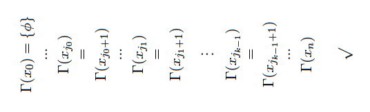
Figure 10: TRANSITIONS in $b$: view sideways

If $b$ ends in a tick from EMPTY then let $S=\{0,1,2,...,k\}$: so it contains $k+1$ states. It is convenient to consider that $j_{k}=n$ in the EMPTY case and put $\Gamma(x_{j_{k}})=\{\}$. The states will correspond to $x_{j_{0}},x_{j_{1}},...,x_{j_{k-1}},x_{j_{k}}$.

See Figure 11.

Figure 11: $b$ ends in a tick from EMPTY

If $b$ ends in a tick from LOOP then let $S=\{0,1,2,...,k-1\}$: so it contains $k$ states. These will correspond to $x_{j_{0}},x_{j_{1}},...,x_{j_{k-1}}$.

See Figure 12.

Figure 12: $b$ ends in a tick from LOOP

Let $R$ contain each $(i,i+1)$ for $i<k-1$. We will also add extra pairs to $R$ to make a fullpath.

If $b$ ends in a tick from EMPTY then just put $(k-1,k)$ and a self-loop $(k,k)$ in $R$ as well. See Figure 13.

Figure 13: $b$ ends in a tick from EMPTY

If $b$ ends in a tick from LOOP then just put $(k-1,l)$ in $R$ as well where $l$ is as follows. Say that $x_{m}$ is the state that “matches” $x_{n}$. So look at the application of the LOOP rule that ended $b$ in a tick. There is a proper ancestor $x_{m}$ of $x_{n}$ in the tableau with $\Gamma(x_{m})\supseteq\Gamma(x_{n})$ and all eventualities in $\Gamma(x_{m})$ are cured between $x_{m}$ and $x_{n}$. The rule requires $x_{m}$ to be poised so it is just before a TRANSITION rule. So say that $m=j_{l}$. Put $(k-1,l)\in R$. See Figure 14.

Figure 14: $m=j_{l}$

A model with a line and one loop back is sometimes called a lasso [SC85].

Now let us define the labelling $g$ of states by atoms in $(S,R,g)$. Let $g(i)=\{p\in AP|p\in\Gamma(x_{j_{i}})\}$.

Finally our proposed model of $\phi$ is along the only fullpath $\sigma$ of $(S,R,g)$ that starts at $0$. That is, if $b$ ends in a tick from EMPTY then $\sigma=\langle 0,1,2,...,k-1,k,k,k,k,...\rangle$ while if $b$ ends in a tick from LOOP then $\sigma=\langle 0,1,2,...,k-2,k-1,l,l+1,l+2,...,k-2,k-1,l,l+1,...\rangle$.

Let $N$ be the length of the first (non-repeating) part of the model: in the EMPTY case $N=k-1$ and in the LOOP case $N=l$. Let $M$ be the length of the repeating part: in the EMPTY case $M=1$ and in the LOOP case $N=k-l$. So in either case the model has $N+M$ states $\{0,1,...,N+M-1\}$ with state $N$ coming (again) after state $N+M-1$ etc. In particular, $\sigma_{i}=i$ for $i<N$ and $\sigma_{i}=(i-N)\bmod M+N$ otherwise.

Now we are going to define a set $\Delta_{i}$ of formulas for each $i=0,1,2,....$, that we will want to be satisfied at $\sigma_{i}$. They collect formulas in labels in between TRANSITIONS, and loop on forever. Thus $\Delta_{0}$ is to be a set of formulas that we want to be true at the first state of the model and $\Delta_{N}$ those true when the model starts to repeat. In the very special case of $N=0$, when $0$ is the first repeating state, let $\Delta_{0}=\bigcup_{s\leq j_{0}}\Gamma(x_{s})\cup\bigcup_{j_{k-1}<s\leq n}\Gamma(x_{s})$. If $N>0$ then let the collection for the first repeating state be $\Delta_{N}=\bigcup_{j_{N-1}<s\leq j_{N}}\Gamma(x_{s})\cup\bigcup_{j_{k-1}<s\leq n}\Gamma(x_{s})$. So in either case, $\Delta_{N}$ has formulas from two separate sections of the tableau.

If $N>0$, for $i=0$, put $\Delta_{0}=\bigcup_{s\leq j_{0}}\Gamma(x_{s})$. For each $i=1,2,...,N+M-1$, except $i=N$, let $\Delta_{i}=\bigcup_{j_{i-1}<s\leq j_{j}}\Gamma(x_{s})$, all the formulas that appear between the $(i-1)th$ and $i$th consecutive uses of the TRANSITION rule.

Finally, for all $i\geq N+M$, put $\Delta_{i}=\Delta_{i-M}=\Delta_{(i-N)\bmod M+N}$.

LEMMA 1

If $X\alpha\in\Delta_{i}$ for some $i$, then $\alpha\in\Delta_{i+1}$. Also, if $\neg X\alpha\in\Delta_{i}$ for some $i$, then $\neg\alpha\in\Delta_{i+1}$.

PROOF: Just consider the $X\alpha$ case: the $\neg X\alpha$ case is similar.

Choose some $i$ such that $X\alpha\in\Delta_{i}$. As the $\Delta_{i}$s repeat, we may as well assume $0\leq i\leq N+M-1$. There are three main cases: $i=N$, $i=N+M-1$ or otherwise.

Consider the $i\neq N$ and $i\neq N+M-1$ case first. Thus $X\alpha$ appears in some $\Gamma(x_{s})$ for $j_{i-1}<s\leq j_{i}$. Because no static rules remove them, any formula of the form $X\alpha$ will survive in the tableau labels until the poised label $\Gamma(x_{j_{i}})$ just before a TRANSITION rule is used. After the TRANSITION rule we will have $\alpha\in\Gamma(x_{j_{i}+1})$ and $\alpha$ will be collected in $\Delta_{i+1}$, the next state label collection.

However, in the other case when $i=N+M-1$, we have $X\alpha$ surviving to be in the poised label $\Gamma(x_{j_{N+M-1}})$. In that case, $\alpha$ will be in $\Gamma(x_{j_{N+M-1}+1})$ and collected in $\Delta_{N}$. But, when $i=N+M-1$ then $i+1=N+M$ and so $\Delta_{i+1}=\Delta_{N+M}=\Delta_{N}\ni\alpha$ as required.

Finally, in the case when $i=N$, we may have $X\alpha$ in some $\Gamma(x_{s})$ for $j_{N-1}<s\leq j_{N}$ or in some $\Gamma(x_{s})$ for $j_{k-1}<s\leq j_{n}$. In the first subcase, it survives until $\Gamma(x_{N})$ and the reasoning proceeds as above. In the second subcase, $X\alpha\in\Gamma(x_{s})$ for some $s$ with $j_{k-1}<s\leq j_{n}$. Thus it survives to be in $\Gamma(x_{j_{n}})$ when we are about to use the LOOP rule. However, it will then also be in $\Gamma(x_{j_{l}})\supseteq\Gamma(x_{n})$. After the TRANSITION rule at $x_{j_{l}}=x_{j_{N}}$, $\alpha$ will be in $\Gamma(x_{j_{N}+1})$ and will be collected in $\Delta_{N+1}$ as required. $\square$

LEMMA 2

Suppose $\alpha U\beta\in\Delta_{i}$. Then there is some $d\geq i$ such that $\beta\in\Delta_{d}$ and for all $f$, if $i\leq f<d$ then $\{\alpha,\alpha U\beta,X(\alpha U\beta)\}\subseteq\Delta_{f}$.

PROOF: For all $i$, whenever $\alpha U\beta\in\Delta_{i}$ then either $\beta$ will also be there or both $\alpha$ and $X(\alpha U\beta)$ will be. To see this, consider which static rules can be used to remove $\alpha U\beta$. Only the $U-$ and $F$-rule can do this.

By Lemma 1, if $X(\alpha U\beta)\in\Delta_{i}$ then $\alpha U\beta\in\Delta_{i+1}$. Thus, by a simple induction, $\alpha U\beta$, and so also the other two formulas, will be in all $\Delta_{f}$ for $f\geq i$ unless $f\geq d\geq i$ with $\beta\in\Delta_{d}$.

It remains to show that $\beta$ does appear in some $\Delta_{d}$.

If the branch ended with EMPTY, then we know this must happen as the $\Gamma(x_{n})$ is empty and so does not contain $X(\alpha U\beta)$. So suppose that the branch ended with a LOOP up to tableau node $x_{j_{l}}$ but that $\alpha U\beta\in\Delta_{f}$ for all $f\geq i$.

For some $f>i$, we have $(f-N)\bmod M=0$, so we know $\alpha U\beta\in\Delta_{f}=\Gamma(x_{j_{l}})$. Thus $\alpha U\beta$ is one of the eventualities in $\Gamma(x_{j_{l}})$ that have to be satisfied between $x_{j_{l}}$ and $x_{n}$.

Say that $\beta\in\Gamma(x_{h})$ and it will also be in the next pre-TRANSITION label $x_{j_{q}}$ after $x_{h}$. So eventually we find a $d\geq i$ such that $(d-N)\bmod M+N=q$ and $\beta\in\Delta_{d}$ as required. $\square$

LEMMA 3

Suppose $\neg(\alpha U\beta)\in\Delta_{i}$. Then either 1) or 2) hold. 1) There is some $d\geq i$ such that $\neg\alpha,\neg\beta\in\Delta_{d}$ and for all $f$, if $i\leq f<d$ then $\{\neg\beta,\neg(\alpha U\beta),X\neg(\alpha U\beta)\}\subseteq\Delta_{f}$. 2) For all $d\geq i$, $\{\neg\beta,\neg(\alpha U\beta),X\neg(\alpha U\beta)\}\subseteq\Delta_{d}$.

PROOF: This is similar to Lemma 2. $\square$

Now we need to show that $(S,R,g),\sigma\models\phi$. To do so we prove a stronger result: a truth lemma.

LEMMA 4 (truth lemma)

for all $\alpha$, for all $i\geq 0$, if $\alpha\in\Delta_{i}$ then $(S,R,g),\sigma_{\geq i}\models\alpha$.

PROOF: This is proved by induction on the construction of $\alpha$. However, we do cases for $\alpha$ and $\neg\alpha$ together and prove that for all $\alpha$, for all $i\geq 0$: if $\alpha\in\Delta_{i}$ then $(S,R,g),\sigma_{\geq i}\models\alpha$; and if $\neg\alpha\in\Delta_{i}$ then $(S,R,g),\sigma_{\geq i}\models\neg\alpha$.

The case by case reasoning is straightforward given the preceeding lemmas. See the long version for details.

Case $p$: Fix $i\geq 0$. If $i<N$ let $i^{\prime}=i$ and otherwise let $i^{\prime}=(i-N)\bmod M+N$. Thus $\sigma_{i}=i^{\prime}$. If $p\in\Delta_{i}=\Gamma(x_{j_{i^{\prime}}})$ then, by definition of $g$, $p\in g(i^{\prime})$. So $p\in g(\sigma_{i})$ and $(S,R,g),\sigma_{\geq i}\models p$ as required. If $\neg p\in\Delta_{i}$ then (by rule CONTRADICTION) we did not put $p$ in $g(i^{\prime})$ and thus $(S,R,g),\sigma_{\geq i}\models\neg p$. This follows as no static rules remove atoms or negated atoms from labels.

Case $\neg\neg\alpha$: Fix $i\geq 0$. If $\neg\neg\alpha\in\Delta_{i}$ then $(S,R,g),\sigma_{\geq i}\models\neg\neg\alpha$ because $\alpha$ will also have been put in $\Delta_{i}$ (by the $\neg\neg$-rule) and so by induction $(S,R,g),\sigma_{\geq i}\models\alpha$. Note that the $\bot$-rule also removes a double negation from a label set but it immediately crosses the branch so it is not relevant here. $\neg\neg\neg\alpha$ is similar.

Case $\alpha\wedge\beta$: Fix $i\geq 0$. Suppose $\alpha\wedge\beta\in\Delta_{i}$. We know this formula is removed before the next TRANSITION (or the end of the branch if that is sooner). There are two ways for such a conjunction to be removed: the $\wedge$-rule, or if the optional $\leftrightarrow$-rule is able to applied and is used. In the first case $(S,R,g),\sigma_{\geq i}\models\alpha\wedge\beta$ because $\alpha$ and $\beta$ will also have been put in $\Delta_{i}$ (by the $\wedge$-rule) and so by induction $(S,R,g),\sigma_{\geq i}\models\alpha$ and $(S,R,g),\sigma_{\geq i}\models\beta$.

Suppose instead that $\alpha=\alpha_{1}\rightarrow\beta_{1}$ and $\beta=\beta_{1}\rightarrow\alpha_{1}$ and the $\leftrightarrow$-rule is used to remove $\alpha\wedge\beta$. Then on branch $b$ either $\alpha_{1}$ and $\beta_{1}$ are included and so in $\Delta_{i}$ as well, or their negations are. In the first case, by induction we have $(S,R,g),\sigma_{\geq i}\models\alpha_{1}$ and $(S,R,g),\sigma_{\geq i}\models\beta_{1}$, and so we also have $(S,R,g),\sigma_{\geq i}\models\alpha_{1}\rightarrow\beta_{1}$ and $(S,R,g),\sigma_{\geq i}\models\beta_{1}\rightarrow\alpha_{1}$ as required. The second negated case is similar.

Suppose $\neg(\alpha\wedge\beta)\in\Delta_{i}$. Again we know this formula is removed and we see that there are four rules that could cause that to happen: $\neg\wedge$-rule, $\top$-rule, $\vee$-rule and $\rightarrow$-rule.

If $\neg(\alpha\wedge\beta)\in\Delta_{i}$ is removed by $\neg\wedge$-rule then $(S,R,g),\sigma_{\geq i}\models\neg(\alpha\wedge\beta)$ because we will have put $\neg\alpha\in\Delta_{i}$ or $\neg\beta\in\Delta_{i}$ (or one or both of them are already there) and so by induction $(S,R,g),\sigma_{\geq i}\models\neg\alpha$ or $(S,R,g),\sigma_{\geq i}\models\neg\beta$.

$\top$-rule: If $\top=\neg(\neg p\wedge\neg\neg p)\in\Delta_{i}$ is removed by $\top$-rule then $(S,R,g),\sigma_{\geq i}\models\neg(\neg p\wedge\neg\neg p)$ anyway so we are done.

$\vee$-rule: If $\alpha\vee\beta=\neg(\neg\alpha\wedge\neg\beta)\in\Delta_{i}$ is removed by $\vee$-rule then $(S,R,g),\sigma_{\geq i}\models\neg(\neg\alpha\wedge\neg\beta)$ because we will have put $\alpha\in\Delta_{i}$ or $\beta\in\Delta_{i}$ (or one or both of them are already there) and so by induction $(S,R,g),\sigma_{\geq i}\models\alpha$ or $(S,R,g),\sigma_{\geq i}\models\beta$.

$\rightarrow$-rule: If $\alpha\rightarrow\beta=\neg(\neg\neg\alpha\wedge\neg\beta)\in\Delta_{i}$ is removed by $\rightarrow$-rule then $(S,R,g),\sigma_{\geq i}\models\neg(\neg\neg\alpha\wedge\neg\beta)$ because we will have put $\neg\alpha\in\Delta_{i}$ or $\beta\in\Delta_{i}$ (or one or both of them are already there) and so by induction $(S,R,g),\sigma_{\geq i}\models\neg\alpha$ or $(S,R,g),\sigma_{\geq i}\models\beta$.

Case $\alpha U\beta$: If $\alpha U\beta\in\Delta_{i}$ then by the $U$-rule, or the optional $F$-rule, we will have either put both $\alpha\in\Delta_{i}$ and $X(\alpha U\beta)\in\Delta_{i}$ or we will have $\beta\in\Delta_{i}$.

Consider the second case. $(S,R,g),\sigma_{\geq i}\models\beta$ so $(S,R,g),\sigma_{\geq i}\models\alpha U\beta$ and we are done.

Now consider the first case: $\alpha U\beta\in\Delta_{i}$ as well as $\alpha\in\Delta_{i}$ and $X(\alpha U\beta)\in\Delta_{i}$. By Lemma 2, this keeps being true for later $i^{\prime}\geq i$ until $\beta\in\Delta_{i^{\prime}}$. By induction, for each $i^{\prime}\geq i$ until then, $(S,R,g),\sigma_{\geq{i^{\prime}}}\models\alpha$. Clearly if we get to a $l>i$ with $\beta\in\Delta_{l}$ then $(S,R,g),\sigma_{\geq{l}}\models\beta$ and $(S,R,g),\sigma_{\geq{i}}\models\alpha U\beta$ as required.

If $\neg(\alpha U\beta)\in\Delta_{i}$ then $\neg U$-rule and $G$-rule mean that $\neg\beta,\neg\alpha\in\Delta_{i}$ or $\neg\beta,X\neg(\alpha U\beta)\in\Delta_{i}$.

In the first case, $(S,R,g),\sigma_{\geq i}\models\neg\alpha$ and $(S,R,g),\sigma_{\geq i}\models\neg\beta$ so $(S,R,g),\sigma_{\geq i}\models\neg(\alpha U\beta)$ as required.

In the second case we can use Lemma 3 which uses an induction to show that $\neg\beta$, $\neg(\alpha U\beta)$, $X\neg(\alpha U\beta)$ keep appearing in the $\Delta_{i^{\prime}}$ labels forever or until $\neg\alpha$ also appears.

In either case $(S,R,g),\sigma_{\geq i}\models\neg(\alpha U\beta)$ as required.

Case $X\alpha$: If $X\alpha\in\Delta_{i}$ then, by Lemma 1 $\alpha\in\Delta_{i+1}$ so by induction $(S,R,g),\sigma_{\geq i+1}\models\alpha$ and $(S,R,g),\sigma_{\geq i}\models X\alpha$ as required.

$\neg X\alpha$ is similar. If $\neg X\alpha\in\Delta_{i}$ then, by Lemma 1, $\neg\alpha\in\Delta_{i+1}$ so by induction (because we did $\neg\alpha$ first) $(S,R,g),\sigma_{\geq i+1}\models\neg\alpha$ and $(S,R,g),\sigma_{\geq i}\models\neg X\alpha$ as required.

And thus ends the soundness proof. $\square$

If we have a successful tableau then the formula is satisfiable.

Notice that the PRUNE rules play no part in the soundness proof. A ticked branch encodes a model even if a PRUNE rule is not applied when it could be.

8 Proof of Completeness:

We have to show that if a formula has a model then it has a successful tableau. This time we will use the model to find the tableau. The basic idea is to use a model (of the satisfiable formula) to show that in any tableau there will be a branch (i.e. a leaf) with a tick.

A weaker result is to show that there is some tableau with a leaf with a tick. Such a weaker result may actually be ok to establish correctness and complexity of the tableau technique. However, it raises questions about whether a “no” answer from a tableau is correct and it does not give clear guidance for the implementer. We show the stronger result: it does not matter which order static rules are applied.

LEMMA 5 (Completeness)

Suppose that $\phi$ is a satisfiable formula of LTL. Then any finished tableau for $\phi$ will be successful.

PROOF: Suppose that $\phi$ is a satisfiable formula of LTL. It will have a model. Choose one, say $(S,R,g),\sigma\models\phi$. In what follows we (use standard practice when the model is fixed and) write $\sigma_{\geq i}\models\alpha$ when we mean $(S,R,g),\sigma_{\geq i}\models\alpha$.

Also, build a completed tableau $T$ for $\phi$ in any manner as long as the rules are followed. Let $\Gamma(x)$ be the formula set label on the node $x$ in $T$. We will show that $T$ has a ticked leaf.

To do this we will construct a sequence $x_{0},x_{1},x_{2},....$ of nodes, with $x_{0}$ being the root. This sequence may terminate at a tick (and then we have succeeded) or it may hypothetically go on forever (and more on that later). In general, the sequence will head downwards from a parent to a child node but occasionally it may jump back up to an ancestor.

As we go we will make sure that each node $x_{i}$ is associated with an index $J(i)$ along the fullpath $\sigma$ and we guarantee the following invariant $INV(x_{i},J(i))$ for each $i\geq 0$. The relationship $INV(x,j)$ is that for each $\alpha\in\Gamma(x)$, $\sigma_{\geq j}\models\alpha$.

Start by putting $J(0)=0$ when $x_{0}$ is the tableau root node. Note that the only formula in $\Gamma(x_{0})$ is $\phi$ and that $\sigma_{\geq 0}\models\phi$. Thus $INV(x_{0},J(0))$ holds at the start.

Now suppose that we have identified the $x$ sequence up until $x_{i}$. Consider the rule that is used in $T$ to extend a tableau branch from $x_{i}$ to some children. Note that we can also ignore the cases in which the rule is EMPTY or LOOP because they would immediately give us the ticked branch that is sought.

It is useful to define the sequence advancement procedure in the cases apart from the PRUNE rules separately. Thus we now describe a procedure, call it $A$, that is given a node $x$ and index $j$ satisfying $INV(x,j)$ and, in case that the node $x$ has children via any rule except PRUNE, the procedure $A$ will give us a child node $x^{\prime}$ and index $j^{\prime}$ which is either $j$ or $j+1$, such that $INV(x^{\prime},j^{\prime})$ holds. The idea will be to use procedure $A$ on $x_{i}$ and $J(i)$ to get $x_{i+1}$ and $J(i+1)$ in case the PRUNE rule is not used at node $x_{i}$. We return to deal with advancing from $x_{i}$ in case that a PRUNE rule is used later. So now we describe procedure $A$ with $INV(x,j)$ assumed.

[EMPTY] If $\Gamma(x)=\{\}$ then we are done. $T$ is a successful tableau as required.

[CONTRADICTION] Consider if it is possible for us to reach a leaf at $x$ with a cross because of a contradiction. So there is some $\alpha$ with $\alpha$ and $\neg\alpha$ in $\Gamma(x)$. But this can not happen as then $\sigma_{\geq j}\models\alpha$ and $\sigma_{\geq j}\models\neg\alpha$.

[$\neg\neg$-rule] So $\neg\neg\alpha$ is in $\Gamma(x)$ and there is one child, which we will make $x^{\prime}$ and we will put $j^{\prime}=j$. Because $\sigma_{\geq j}\models\neg\neg\alpha$ we also have $\sigma_{\geq j^{\prime}}\models\alpha$. Also for every other $\beta\in\Gamma(x^{\prime})\subseteq\Gamma(x)\cup\{\alpha\}$, we still have $\sigma_{\geq j^{\prime}}\models\beta$. So we have the invariant holding.

[$\wedge$-rule] So $\alpha\wedge\beta$ is in $\Gamma(x)$ and there is one child, which we will make $x^{\prime}$ and we will put $j^{\prime}=j$. Because $\sigma_{\geq j}\models\alpha\wedge\beta$ we also have $\sigma_{\geq j^{\prime}}\models\alpha$ and $\sigma_{\geq j^{\prime}}\models\beta$. Also for every other $\gamma\in\Gamma(x^{\prime})\subseteq\Gamma(x_{i})\cup\{\alpha,\beta\}$, we still have $\sigma_{\geq j^{\prime}}\models\gamma$. So we have the invariant holding.

[$\neg\wedge$-rule] So $\neg(\alpha\wedge\beta)$ is in $\Gamma(x)$ and there are two children. One $y$ is labelled $(\Gamma(x)\setminus\{\neg(\alpha\wedge\beta)\})\cup\{\neg\alpha\}$ and the other, $z$, is labelled $(\Gamma(x)\setminus\{\neg(\alpha\wedge\beta)\})\cup\{\neg\beta\}$. We know $\sigma_{\geq j}\models\neg(\alpha\wedge\beta)$. Thus, $\sigma_{\geq j}\not\models\alpha\wedge\beta$ and it is not the case that both $\sigma_{\geq j}\models\alpha$ and $\sigma_{\geq j}\models\beta$. So either $\sigma_{\geq j}\models\neg\alpha$ or $\sigma_{\geq j}\models\neg\beta$.

If the former, i.e. that $\sigma_{\geq j}\models\neg\alpha$ we will make $x^{\prime}=y$ and otherwise we will make $x^{\prime}=z$. In either case put $j^{\prime}=j$. Let us check the invariant. Consider the first case. The other is exactly analogous.

We already know that we have $\sigma_{\geq j^{\prime}}\models\neg\alpha$. Also for every other $\gamma\in\Gamma(x^{\prime})=\Gamma(y)\subseteq\Gamma(x)\cup\{\neg\alpha\}$, we still have $\sigma_{\geq j^{\prime}}\models\gamma$. So we have the invariant holding.

[$U$-rule] So $\Gamma(x)=\Delta\mathbin{\mathaccent 0{\cdot}\cup}\{\alpha U\beta\}$ and there are two children. One $y$ is labelled $\Gamma(y)=\Delta\cup\{\beta\}$ and the other, $z$, is labelled $\Gamma(z)=\Delta\cup\{\alpha,X(\alpha U\beta)\}$. We know $\sigma_{\geq j}\models\alpha U\beta$. Thus, there is some $k\geq j$ such that $\sigma_{\geq k}\models\beta$ and for all $l$, if $j\leq l<k$ then $\sigma_{\geq l}\models\alpha$. If $\sigma_{\geq j}\models\beta$ then we can choose $k=j$ (even if other choices as possible) and otherwise choose any such $k>j$. Again there are two cases, either $k=j$ or $k>j$.

In the first case, when $\sigma_{\geq j}\models\beta$, we put $x^{\prime}=y$ and otherwise we will make $x^{\prime}=z$. In either case put $j^{\prime}=j$.

Let us check the invariant. Consider the first case. We have $\sigma_{\geq j^{\prime}}\models\beta$.

In the second case, we know that we have $\sigma_{\geq j^{\prime}}\models\alpha$ and $\sigma_{\geq j^{\prime}+1}\models\alpha U\beta$. Thus $\sigma_{\geq j^{\prime}}\models X(\alpha U\beta)$.

Also, in either case, for every other $\gamma\in\Gamma(x^{\prime})$ we still have $\sigma_{\geq j^{\prime}}\models\gamma$. So we have the invariant holding.

[$\neg U$-rule] So $\Gamma(x)=\Delta\mathbin{\mathaccent 0{\cdot}\cup}\{\neg(\alpha U\beta)\}$ and there are two children. One $y$ is labelled $\Delta\cup\{\neg\alpha,\neg\beta\}$ and the other, $z$, is labelled $\Delta\cup\{\neg\beta,X\neg(\alpha U\beta)\}$. We know $\sigma_{\geq j}\models\neg(\alpha U\beta)$. So for sure $\sigma_{\geq j}\models\neg\beta$.

Furthermore, possibly $\sigma_{\geq j}\models\neg\alpha$ as well, but otherwise if $\sigma_{\geq j}\models\alpha$ then we can show that we can not have $\sigma_{\geq j+1}\models\alpha U\beta$. Suppose for contradiction that $\sigma_{\geq j}\models\alpha$ and $\sigma_{\geq j+1}\models\alpha U\beta$. Then there is some $k\geq j$ such that $\sigma_{\geq k}\models\beta$ and for all $l$, if $j\leq l<k$ then $\sigma_{\geq l}\models\alpha$. Thus $\sigma_{\geq j}\models\alpha U\beta$. Contradiction.

So we can conclude that there are two cases when the $\neg U$-rule is used. CASE 1: $\sigma_{\geq j}\models\neg\beta$ and $\sigma_{\geq j}\models\neg\alpha$. CASE 2: $\sigma_{\geq j}\models\neg\beta$ and $\sigma_{\geq j+1}\models\neg(\alpha U\beta)$.

In the first case, when $\sigma_{\geq j}\models\neg\beta$, we put $x^{\prime}=y$ and otherwise we will make $x^{\prime}=z$. In either case put $j^{\prime}=j$.

Let us check the invariant. In both cases we know that we have $\sigma_{\geq j^{\prime}}\models\neg\beta$. Now consider the first case. We also have $\sigma_{\geq j}\models\neg\alpha$. In the second case, we know that we have $\sigma_{\geq j+1}\models\neg(\alpha U\beta)$. Thus $\sigma_{\geq j^{\prime}}\models X\neg(\alpha U\beta)$. Also, in either case, for every other $\gamma\in\Gamma(x^{\prime})$ we still have $\sigma_{\geq j^{\prime}}\models\gamma$. So we have the invariant holding.

[OTHER STATIC RULES]: similar.

[TRANSITION] So $\Gamma(x)$ is poised and there is one child, which we will make $x^{\prime}$ and we will put $j^{\prime}=j+1$.

Consider a formula $\gamma\in\Gamma(x^{\prime})=\{\alpha|X\alpha\in\Gamma(x)\}\cup\{\neg\alpha|\neg X\alpha\in\Gamma(x)\}$.

CASE 1: Say that $X\gamma\in\Gamma(x)$. Thus, by the invariant, $\sigma_{\geq j}\models X\gamma$. Hence, $\sigma_{\geq j+1}\models\gamma$. But this is just $\sigma_{\geq j^{\prime}}\models\gamma$ as required.

CASE 2: Say that $\gamma=\neg\delta$ and $\neg X\delta\in\Gamma(x)$. Thus, by the invariant, $\sigma_{\geq j}\models\neg X\delta$. Hence, $\sigma_{\geq j+1}\not\models\delta$. But this is just $\sigma_{\geq j(i+1)}\models\gamma$ as required.

So we have the invariant holding.

[LOOP] If, in $T$, the node $x_{i}$ is a leaf just getting a tick via the LOOP rule then we are done. $T$ is a successful tableau as required.

So that ends the description of procedure $A$ that is given a node $x$ and index $j$ satisfying $INV(x,j)$ and, in case that the node $x$ has children via any rule except PRUNE or PRUNE₀, the procedure $A$ will give us a child node $x^{\prime}$ and index $j^{\prime}$, which is either $j$ or $j+1$, such that $INV(x^{\prime},j^{\prime})$ holds. We use procedure $A$ to construct a sequence $x_{0},x_{1},x_{2},....$ of nodes, with $x_{0}$ being the root. and guarantee the invariant $INV(x_{i},J(i))$ for each $i\geq 0$.

The idea will be to use procedure $A$ on $x_{i}$ and $J(i)$ to get $x_{i+1}$ and $J(i+1)$ in case the PRUNE rule is not used at node $x_{i}$. Start by putting $J(0)=0$ when $x_{0}$ is the tableau root node. We have seen that $INV(x_{0},J(0))$ holds at the start.

[PRUNE ] Now, we complete the description of the construction of the $x_{i}$ sequence by explaining what to do in case $x_{i}$ is a node on which PRUNE is used. Suppose that $x_{i}$ is a node which gets a cross in $T$ via the PRUNE rule. So there is a sequence $u=x_{h},x_{h+1},...,x_{h+a}=v,x_{h+a+1},...,x_{h+a+b}=x_{i}=w$ such that $\Gamma(u)=\Gamma(v)=\Gamma(w)$ and no extra eventualities of $\Gamma(u)$ are satisfied between $v$ and $w$ that were not already satisfied between $u$ and $v$.

What we do now is to undertake a sort of backtracking exercise in our proof. We choose some such $u$, $v$ and $w$, there may be more than one triple, and proceed with the construction as if $x_{i}$ was $v$ instead of $w$. That is we use the procedure $A$ on $v$ with $J(i)$ to get from $v$ to one $x_{i+1}$ of its children and define $J(i+1)$. Procedure $A$ above can be applied because $\Gamma(v)=\Gamma(x_{i})$ and so the invariant holds for $v$ with $J(i)$ as well as for $x_{i}$ with $J(i)$.

Thus we keep going with the new $x_{i+1}$ child of $v$, and $J(i)$.

If the variant PRUNE₀ rule is used on $x_{i}$ then the action is similar but simpler. So there is a sequence $u=x_{h},x_{h+1},...,x_{h+a}=x_{i}=v$ such that $\Gamma(u)=\Gamma(v)$ and no eventualities of $\Gamma(u)$ are satisfied between $u$ and $v$ but there is at least one eventuality in $\Gamma(u)$.

What we do now is to choose some such $u$, and $v$, and proceed with the construction as if $x_{i}$ was $u$ instead of $v$. That is we use the procedure $A$ on $u$ with $J(i)$ to get from $u$ to one $x_{i+1}$ of its children and define $J(i+1)$. Procedure $A$ above can be applied because $\Gamma(u)=\Gamma(x_{i})$ and so the invariant holds for $u$ with $J(i)$ as well as for $x_{i}$ with $J(i)$. Thus we keep going with the new $x_{i+1}$ child of $u$, and $J(i)$.

Now let us consider whether the above construction goes on for ever. Clearly it may end finitely with us finding a ticked leaf and succeeding. However, at least in theory, it may seem possible that the construction keeps going forever even though the tableau will be finite. The rest of the proof is to show that this actually can not happen. The construction can not go on forever. It must stop and the only way that we have shown that that can happen is by finding a tick.

Suppose for contradiction that the construction does go on forever. Thus, because there are only a finite number of nodes in the tableau, we must meet the PRUNE (or PRUNE₀) rule and jump back up the tableau infinitely often.

When we do find an application of the PRUNE rule with triple $(u,v,w)$ of nodes from $T$ call that a jump triple. Similarly, when we find an application of the PRUNE₀ rule with pair $(u,v)$ of nodes from $T$ call that a jump pair. Let jump tuples be either jump pairs or jump triples.

There are only a finite number of jump tuples so there must be some that cause us to jump infinitely often. Call these recurring jump tuples.

Say that $(u_{0},v_{0},w_{0})$ or $(u_{0},v_{0})$ is one such. We can choose $u_{0}$ so that for no other recurring jump triple $(u_{1},v_{1},w_{1})$ or pair $(u_{1},v_{1})$ do we have $u_{1}$ being a proper ancestor of $u_{0}$.

As we proceed through the construction of $x_{0},x_{1},..$ and see a jump every so often, eventually all the jump tuples who only cause a jump a finite number of times stop causing jumps. After that time, $(u_{0},v_{0},w_{0})$ or $(u_{0},v_{0})$ will still cause a jump every so often.

Thus after that time $u_{0}$ will never appear again as the $x_{i}$ that we choose and all the $x_{i}$s that we choose will be descendants of $u_{0}$. This is because we will never jump up to $u_{0}$ or above it (closer to the root). Say that $x_{N}$ is the very last $x_{i}$ that is equal to $u_{0}$.

Now consider any $X(\alpha U\beta)$ that appears in $\Gamma(u_{0})$. (There must be at least one eventuality in $\Gamma(u_{0})$ as it is used to apply rule PRUNE or PRUNE₀).

A simple induction shows that $\alpha U\beta$ or $X(\alpha U\beta)$ will appear in every $\Gamma(x_{i})$ from $i=N$ up until at least when $\beta$ appears in some $\Gamma(x_{i})$ after that (if that ever happens). This is because if $\alpha U\beta$ is in $\Gamma(x_{i})$ and $\beta$ is not there and does not get put there then $X(\alpha U\beta)$ will also be put in before the next temporal TRANSITION rule. Each temporal TRANSITION rule will thus put $\alpha U\beta$ into the new label. Finally, in case the $x_{i}$ sequence meets a PRUNE jump $(u,v,w)$ then the new $x_{i+1}$ will be a child of $v$ which is a descendent of $u$ which is a descendent of $u_{0}$ so will also contain $\alpha U\beta$ or $X(\alpha U\beta)$. Similarly with PRUNE₀ jumps.

Now $J(i)$ just increases by $0$ or $1$ with each increment of $i$, We also know that $\sigma_{\geq J(i)}\models\alpha U\beta$ from $i=N$ onwards until (and if) $\beta$ gets put in $\Gamma(x_{i})$. Since $\sigma$ is a fullpath we will eventually get to some $i$ with $\sigma_{\geq J(i)}\models\beta$. In that case our construction makes us put $\beta$ in the label. Thus we do eventually get to some $i\geq N$ with $\beta\in\Gamma(x_{i})$. Let $N_{\beta}$ be the first such $i\geq N$. Note that all the nodes between $u_{0}$ and $x_{N_{\beta}}$ in the tableau also appear as $x_{i}$ for $N<i<N_{\beta}$ so that they all have $\alpha U\beta$ and not $\beta$ in their labels $\Gamma(x_{i})$.

Now let us consider if we ever jump up above $x_{N_{\beta}}$ at any TRANSITION of our construction (after $i=N_{\beta}$). In that case there would be a PRUNE jump triple of tableau nodes $u$, $v$ and $w$ governing the first such jump or possibly a PRUNE₀ jump. Consider first a PRUNE jump. Since $u$ is not above $u_{0}$ and $v$ is above $x_{N_{\beta}}$, we must have $\Gamma(u)=\Gamma(v)$ with $X(\alpha U\beta)$ in them and $\beta$ not satisfied in between. But $w$ will be below $x_{N_{\beta}}$ at the first such jump, meaning that $\beta$ is satisfied between $v$ and $w$. That is a contradiction to the PRUNE rule being applicable to this triple.

Now consider a PRUNE₀ jump from $v$ below $x_{N_{\beta}}$ up to $u$ above it. Since $u$ is not above $u_{0}$ and $v$ is below $x_{N_{\beta}}$, we must have $\Gamma(u)=\Gamma(v)$ with $X(\alpha U\beta)$ in them and not satisfied in between. But $v$ will be below $x_{N_{\beta}}$ at the first such jump, meaning that $\beta$ is satisfied between $u$ and $v$. That is a contradiction to the PRUNE₀ rule being applicable to this triple.

Thus the $x_{i}$ sequence stays within descendants of $x_{N_{\beta}}$ forever after $N_{\beta}$.

The above reasoning applies to all eventualities in $\Gamma(u_{0})$. Thus, after they are each satisfied, the construction $x_{i}$ does not jump up above any of them. When the next supposed jump involving $u_{0}$ with some $v$ and (perhaps) $w$ happens after that it is clear that all of the eventualities in $\Gamma(u_{0})$ are satisfied above $v$.

This is a contradiction to such a jump ever happening. Thus we can conclude that there are not an infinite number of jumps after all. The construction must finish with a tick. This is the end of the completeness proof. $\square$

9 Complexity and Implementation

Deciding LTL satisfiability is in PSPACE [SC85]. (In fact our tableau approach can be used to show that via Savitch’s theorem by assuming guessing the right branch.)

The tableau search through the new tableau, even in a non-parallel implementation, should (theoretically) be able to be implemented to run faster than that through the state of the art tableau technique of [Sch98a]. This is because there is less information to keep track of and no backtracking from potentially successful branches when a repeated label is discovered.

A variety of implementations are currently underway at Udine, including some comparative experiments with other available LTLSAT checkers. Early results are very promising and publications on the results will be forthcoming. For now, as this paper is primarily about the theory behind the new rules, we have provided a demonstration Java implementation to allow readers to experiment with the way that the tableau works. The program allows comparison with a corresponding implementation of the Schwendimann tableau. The demonstration Java implementation is available at http://www.csse.uwa.edu.au/~mark/research/Online/ltlsattab.html. This allows users to understand the tableau building process in a step by step way. It is not designed as a fast implementation. However, it does report on ow many tableau construction steps were taken.

Detailed comparisons of the running times are available via the web page. In Figure 15, we give a small selection to give the idea of the experimental results. This is just on a quite long formula, “Rozier 9”, one very long formula “anzu amba amba 6” from the so-called Rozier counter example series of [SD11] and an interesting property “foo4” (described below). Shown is formula length, running time in seconds (on a standard laptop), number of tableau steps and the maximum depth of a branch in poised states. As claimed, on many examples the new tableau needs roughly the same number of steps and the same amount of time on each step. However, there are interesting formulas (such as the foo series) for which the new tableau makes a significant saving.

fmla		Reynolds			Schwendimann
	length	sec	steps	depth	sec	steps	depth
r9	277	109	240k	4609	112	242k	4609
as6	1864	0.001	54	2	0.001	55	2
foo4	84	7.25	7007k	9	15.9	16232k	3

Figure 15: Comparison of the two tableaux from the Java implementation

We use benchmark formulas from the various series described in [SD11]. The only new series we add is $\mbox{foo}_{n}$ as follows: for all $n\geq 2$,

$$\mbox{foo}_{n}=a\wedge G(a\leftrightarrow X\neg a)\wedge\bigwedge_{i=1}^{n}GFb_{i}\wedge\bigwedge_{i=1}^{n}G(b_{i}\rightarrow\neg a)\wedge\bigwedge_{i=1}^{n-1}\bigwedge_{j=i+1}^{n}G\neg(b_{i}\wedge b_{j})$$

Originally, the $\mbox{foo}_{n}$ series was invented by the author to obtain an idea experimentally how much longer it might take the new tableau compared to Schwendimann’s on testing examples but the experiments show the opposite outcome.

10 Comparisons with the Schwendimann Tableau

In this section we give a detailed comparison of the new tableau’s operation compared to that of the Schwendimann’s tableau.

10.1 Schwendimann’s Tableau

From [Sch98a].

The tableau is a labelled tree. Suppose we are to decide the satisfiability or not of $\phi$.

Labels are of the form $(\Gamma,S,R)$ where $\Gamma$ is a set of formulas (subformulas of $\phi$), $S=(Ev,Br)$ is a pair (described shortly) and $R$ is a pair of the form $(n,uev)$ where $n\in N$ and $uev\subseteq cl(\phi)$.

The $\Gamma$ part of a node label $(\Gamma,S,R)$ is a set of subformulas of $\phi$ serving a similar purpose to our node labels.

The second component $S=(Ev,Br)$ is a pair where $Ev$ is a set of formulas, and $Br$ is a list of pairs each of the form $(\Gamma_{i},E_{i})$. The set $Ev$ records the eventualities cured at the current state. The list $Br=\langle(\Gamma_{1},Ev_{1}),...,(\Gamma_{m},Ev_{m})\rangle$ is a record of useful information from the state ancestors of the current node along the current branch. Each $(\Gamma_{i},Ev_{i})$ records the poised label $\Gamma_{i}$ of the $i$th state down the branch and the set $Ev_{i}$ of eventualities fulfilled there.

The second component $S$ essentially contains information about the labels on the current branch of the tree and so is just a different way of managing the same sort of “historical” recording that we manage in our new tableau. We manage the historical records by having the branch ancestor labels directly available for checking.

The third component $(n,uev)$, a pair consisting of a number and a set of formulas, is specific to the Schwendimann tableau process and has no analogous component in our new tableau. The number $n$ records the highest index of ancestor state in the current branch that can be reached directly by an up-link from a descendent node of the current node. The set $uev$ contains the eventualities which are in the current node label but which are not cured by the time of the end of the branch below.

The elements of the third component are not known as the tableau is constructed until all descendants on all branches below the current node are expanded. Then the values can be filled in using some straightforward but slightly lengthy rules about how to compute them from children to parent nodes.

The rules for working out these components are slightly complicated in the case of disjunctive rules, including expansion of $U$ formulas. The third component helps assess when a branch and the whole tableau can be finished.

Apart from having to deal with the second and third components of the labels, the rules are largely similar to the rules for the new tableau. However, there are no prune rules. The Schwendimann tableau does not continue a branch if there is a node with the same label as one of its proper ancestors. The branch stops there.

The other main difference to note is that the Schwendimann tableau construction rules for disjunctive formulas do in general need to combine information from both children’s branches to compute the label on the parent.

10.2 Example

Consider the example

$$\theta=\mbox{foo}_{2}=a\wedge G(a\leftrightarrow X\neg a)\wedge GFb_{1}\wedge GFb_{2}\wedge G(b_{1}\rightarrow\neg a)\wedge G(b_{2}\rightarrow\neg a)\wedge G\neg(b_{1}\wedge b_{2}).$$

Technically Schwendimann tableau assumes all formulas (the input formula and its subformulas) are in negation normal form which involves some rewriting so that negations only appear before atomic propositions. However, we can make a minor modification and assume the static rules are the same as our new ones.

We start a tableau with the label $(\Gamma,S,R)$ with $\Gamma=\{\theta\}$, $S=(\{\},\langle\rangle)$ and $R=(n,uev)$ with both $n$ and $uev$ unknown as yet.

Tableau rules decompose $\theta$ and subsequent subformulas in a similar way to in our new tableau. Neither $S$ nor $R$ change while we do not apply a step rule (known as $X$ rule).

The conjunctions and $G$ rules are just as in our new tableau. Thus the tableau construction soon reaches a node with the label $(\Gamma,S,R)$ as follows: $S=(\{\},\langle\rangle)$, $R=(n,uev)$ with both $n$ and $uev$ unknown as yet and

$$\Gamma=\{a,a\leftrightarrow X\neg a,XG(a\leftrightarrow X\neg a),G(b_{1}\rightarrow\neg a),G(b_{2}\rightarrow\neg a),G\neg(b_{1}\wedge b_{2}),GFb_{1},GFb_{2}\}.$$

There are six choices causing branches within this state caused by the disjuncts and the $F\beta$ formulas. This could lead to 64 different branches before we complete the state but many of these choices lead immediately to contradictions. The details depend on the order of choice of decomposing formulas.

A typical expansion leads to a branch with a node labelled by the state $(\Gamma,S,R)$ as follows: $S=(\{\},\langle\rangle)$, $R=(n,uev)$ with both $n$ and $uev$ unknown as yet and

$$\begin{array}[]{ll}\Gamma_{0}=\{&a,X\neg a,XG(\neg a\leftrightarrow X\neg a),\neg b_{1},XG(b_{1}\rightarrow\neg a),\neg b_{2},\\ &XG(b_{2}\rightarrow\neg a),XG\neg(b_{1}\wedge b_{2}),XFb_{1},XGFb_{1},XFb_{2},XGFb_{2}\}.\end{array}$$

Notice that the first component of $S$ is still empty as, in this case, none of the eventualities, $Fb_{1}$ nor $Fb_{2}$, is fulfilled here.

The next rule to use in such a situation is the transition rule, which is very similar to that in our new tableau, except that the second component part of the label is updated as well. We find $S=(\{\},\langle(\{\},\Gamma_{0})\rangle)$, $R=(n,uev)$ with both $n$ and $uev$ unknown as yet and

$$\Gamma=\{\neg a,G(\neg a\leftrightarrow X\neg a),G(b_{1}\rightarrow\neg a),G(b_{2}\rightarrow\neg a),G\neg(b_{1}\wedge b_{2}),Fb_{1},GFb_{1},Fb_{2},GFb_{2}\}.$$

A further series of expansions and choices leads us to the following new state, $S=(\{b_{1}\},\langle(\{\},\Gamma_{0})\rangle)$, $R=(n,uev)$ with both $n$ and $uev$ unknown as yet and

$$\begin{array}[]{ll}\Gamma_{1}=\{&\neg a,Xa,XG(\neg a\leftrightarrow X\neg a),b_{1},XG(b_{1}\rightarrow\neg a),\neg b_{2},\\ &XG(b_{2}\rightarrow\neg a),XG\neg(b_{1}\wedge b_{2}),XGFb_{1},XFb_{2},XGFb_{2}\}.\end{array}$$

Applying the step rule here gives us the following: $S=(\{\},\langle(\{\},\Gamma_{0}),(\{b_{1}\},\Gamma_{1})\rangle)$, $R=(n,uev)$ with both $n$ and $uev$ unknown as yet and

$$\Gamma=\{a,G(\neg a\leftrightarrow X\neg a),G(b_{1}\rightarrow\neg a),G(b_{2}\rightarrow\neg a),G\neg(b_{1}\wedge b_{2}),Fb_{1},GFb_{1},Fb_{2},GFb_{2}\}.$$

When this is branch is expanded further then we find ourselves at $(\Gamma_{0},S,R)$ with $S=(\{\},\langle(\{\},\Gamma_{0}),(\{b_{1}\},\Gamma_{1})\rangle)$ and $R=(n,uev)$ with both $n$ and $uev$ unknown as yet. Notice the main first part of the label has ended up being $\Gamma_{0}$ again. Thus we have a situation for the LOOP rule.

The loop rule uses the facts that the state repeated has the index $1$ in the branch above and that the eventuality $Fb_{2}$ has not been fulfilled in this branch. Thus we can fill in $n=1$ and $uev=\{Fb_{2}\}$ at all the intervening pre-states which have been left unknown so far. These values do not as yet transfer up to the top state as yet as there are still other undeveloped branches from within that state.

The other two states that we find are a minor variation on $\Gamma_{1}$,

$$\begin{array}[]{ll}\Gamma_{2}=\{&\neg a,Xa,XG(\neg a\leftrightarrow X\neg a),b_{1},XG(b_{1}\rightarrow\neg a),\neg b_{2},\\ &XG(b_{2}\rightarrow\neg a),XG\neg(b_{1}\wedge b_{2}),XFb_{1},XGFb_{1},XFb_{2},XGFb_{2}\},\end{array}$$

and a mirror image of $\Gamma_{1}$ when $b_{2}$ is true instead of $b_{1}$:

$$\begin{array}[]{ll}\Gamma_{3}=\{&\neg a,Xa,XG(\neg a\leftrightarrow X\neg a),\neg b_{1},XG(b_{1}\rightarrow\neg a),b_{2},\\ &XG(b_{2}\rightarrow\neg a),XG\neg(b_{1}\wedge b_{2}),XFb_{1},XGFb_{1},XFb_{2},XGFb_{2}\}.\end{array}$$

Then all eventualities are fulfilled and the tableau succeeds after 3933 steps. The overall picture of states (poised labels) is as follows (with $1$ standing for $\Gamma_{1}$ etc).

10.3 Same Example in New Tableau

By comparison, the new tableau visits the same states but takes only 3087 steps to proceed as follows:

10.4 Comparisons

The new tableau can always decide on the basis of a single branch, working downwards. Schwendimann’s needs communication up and between branches, and will generally require full development of several branches.

The new tableau just needs to store formula labels down current branch. However, if doing depth-first search, also needs information about choices made to enable backtracking. Schwendimann’s tableau needs to pass extra sets of unfulfilled eventualities back up branches also keeping track of indices while backtracking. It also needs to store information about choices made to enable backtracking.

11 Conclusion

We have introduced novel tableau construction rules which support a new tree-shaped, one-pass tableau system for LTLSAT. It is traditional in style, simple in all aspects with no extra notations on nodes, neat to introduce to students, amenable to manual use and promises efficient and fast automation.

In searching or constructing the tableau one can explore down branches completely independently and further break up the search down individual branches into separate independent processes. Thus it is particularly suited to parallel implementations.

Experiments show that, even in a standard depth-first search implementation, it is also competitive with the current state of the art in tableau-based approaches to LTL satisfiability checking. This is good reason to believe that very efficient implementations can be achieved as the step by step construction task is particularly simple and requires on minimal storage and testing.

Because of the simplicity, it also seems to be a good base for more intelligent and sophisticated algorithms: including heuristics for choosing amongst branches and ways of managing sequences of label sets.

The idea of the PRUNE rules potentially have many other applications.

References

- [BA12] Mordechai Ben-Ari. Propositional logic: Formulas, models, tableaux. In Mathematical Logic for Computer Science, pages 7–47. Springer London, 2012.
- [Bet55] E. Beth. Semantic entailment and formal derivability. Mededelingen der Koninklijke Nederlandse Akad. van Wetensch, 18, 1955.
- [CGH97] E. M. Clarke, O. Grumberg, and K. Hamaguchi. Another look at ltl model checking. Formal Methods in System Design, 10(1):47–71, 1997.
- [FDP01] Michael Fisher, Clare Dixon, and Martin Peim. Clausal temporal resolution. ACM Transactions on Computational Logic (TOCL), 2(1):12–56, 2001.
- [Fos95] Ian Foster. Designing and Building Parallel Programs. Addison Wesley, 1995.
- [Gir00] Rod Girle. Modal Logics and Philosophy. Acumen, Teddington, UK, 2000.
- [GKS10] Valentin Goranko, Angelo Kyrilov, and Dmitry Shkatov. Tableau tool for testing satisfiability in ltl: Implementation and experimental analysis. Electronic Notes in Theoretical Computer Science, 262(0):113 – 125, 2010. Proceedings of the 6th Workshop on Methods for Modalities (M4M-6 2009).
- [Gor10] Raj Gore. pltl tableau implementation, 2010.
- [Gou84] G. D. Gough. Decision procedures for temporal logic. Master’s thesis, Department of Computer Science, University of Manchester, 1984.
- [Gou89] G. Gough. Decision procedures for temporal logics. Technical Report UMCS-89-10-1, Department of Computer Science, University of Manchester, 1989.
- [HK03] Ullrich Hustadt and Boris Konev. Trp++ 2.0: A temporal resolution prover. In Automated Deduction–CADE-19, pages 274–278. Springer Berlin Heidelberg, 2003.
- [Hol97] G.J. Holzmann. The model checker SPIN. IEEE Trans. on Software Engineering, Special issue on Formal Methods in Software Practice, 23(5):279–295, 1997.
- [KMMP93] Yonit Kesten, Zohar Manna, Hugh McGuire, and Amir Pnueli. A decision algorithm for full propositional temporal logic. In Costas Courcoubetis, editor, CAV, volume 697 of Lecture Notes in Computer Science, pages 97–109. Springer, 1993.
- [LH10] Michel Ludwig and Ullrich Hustadt. Implementing a fair monodic temporal logic prover. AI Commun., 23(2-3):69–96, 2010.
- [LP85] O. Lichtenstein and A. Pnueli. Checking that finite state concurrent programs satisfy their linear specification. In Proc. 12th ACM Symp. on Princ. Prog. Lang., 1985.
- [LP00] O. Lichtenstein and A. Pnueli. Propositional temporal logic: Decidability and completeness. IGPL, 8(1):55–85, 2000.
- [LWB10] LWB. Lwb tableau implementation, 2010.
- [LZP+13] J. Li, L. Zhang, G. Pu, M. Vardi, and J. He. Ltl satisfiability checking revisited. In TIME 13, 2013.
- [MP95] Zohar Manna and Amir Pnueli. Temporal verification of reactive systems: safety. Springer-Verlag New York, Inc., New York, NY, USA, 1995.
- [Pnu77] A. Pnueli. The temporal logic of programs. In Proceedings of the Eighteenth Symposium on Foundations of Computer Science, pages 46–57, 1977. Providence, RI.
- [Rey11] Mark Reynolds. A tableau-based decision procedure for CTL*. Journal of Formal Aspects of Computing, pages 1–41, August 2011.
- [RV07] Kristin Y. Rozier and Moshe Y. Vardi. Ltl satisfiability checking. In Dragan Bosnacki and Stefan Edelkamp, editors, SPIN, volume 4595 of Lecture Notes in Computer Science, pages 149–167. Springer, 2007.
- [RV11] K. Y. Rozier and M. Y. Vardi. A multi-encoding approach for ltl symbolic satisfiability checking. In 17th International Symposium on Formal Methods (FM2011), volume 6664 of LNCS, pages 417–431. Springer Verlag, 2011.
- [SC85] A. Sistla and E. Clarke. Complexity of propositional linear temporal logics. J. ACM, 32:733–749, 1985.
- [Sch98a] S. Schwendimann. A new one-pass tableau calculus for PLTL. In Harrie C. M. de Swart, editor, Proceedings of International Conference, TABLEAUX 1998, Oisterwijk, LNAI 1397, pages 277–291. Springer, 1998.
- [Sch98b] Stefan Schwendimann. Aspects of Computational Logic. PhD, Institut für Informatik und angewandte Mathematik, 1998.
- [SD11] Viktor Schuppan and Luthfi Darmawan. Evaluating LTL satisfiability solvers. In Tevfik Bultan and Pao-Ann Hsiung, editors, ATVA’11, volume 6996 of Lecture Notes in Computer Science, pages 397–413. Springer, 2011.
- [SGL97] P. Schmitt and J. Goubault-Larrecq. A tableau system for linear-time temporal logic. In TACAS 1997, pages 130–144, 1997.
- [Smu68] R. Smullyan. First-order Logic. Springer, 1968.
- [VW94] M. Vardi and P. Wolper. Reasoning about infinite computations. Information and Computation, 115:1–37, 1994.
- [Wol83] P. Wolper. Temporal logic can be more expressive. Information and computation, 56(1–2):72–99, 1983.
- [Wol85] P. Wolper. The tableau method for temporal logic: an overview. Logique et Analyse, 28:110–111, June–Sept 1985.