$\mathcal{PT}$-Symmetric Model of Immune Response

Abstract

The study of $\mathcal{PT}$-symmetric physical systems began in 1998 as a complex generalization of conventional quantum mechanics, but beginning in 2007 experiments began to be published in which the predicted $\mathcal{PT}$ phase transition was clearly observed in classical rather than in quantum-mechanical systems. This paper examines the $\mathcal{PT}$ phase transition in mathematical models of antigen-antibody systems. A surprising conclusion that can be drawn from these models is that a possible way to treat a serious disease in which the antigen concentration is growing out of bounds (and the host will die) is to inject a small dose of a second (different) antigen. In this case there are two possible favorable outcomes. In the unbroken-$\mathcal{PT}$-symmetric phase the disease becomes chronic and is no longer lethal while in the appropriate broken-$\mathcal{PT}$-symmetric phase the concentration of lethal antigen goes to zero and the disease is completely cured.

I Introduction

There have been many studies of dynamical predator-prey systems that simulate biological processes. Particularly interesting early work was done by Bell R1 , who showed that the immune response can be modeled quite effectively by such systems. In Bell’s work the time evolution of competing concentrations of one antigen and one antibody is studied.

The current paper shows what happens if we combine two antibody-antigen subsystems in a $\mathcal{PT}$-symmetric fashion to make an immune system in which there are two antibodies and two antigens. An unexpected conclusion is that even if one antigen is lethal (because the antigen concentration grows out of bounds), the introduction of a second antigen can stabilize the concentrations of both antigens, and thus save the life of the host. Introducing a second antigen may actually drive the concentration of the lethal antigen to zero.

We say that a classical dynamical system is $\mathcal{PT}$ symmetric if the equations describing the system remain invariant under combined space reflection $\mathcal{P}$ and time reversal $\mathcal{T}$ R2 . Classical $\mathcal{PT}$-symmetric systems have a typical generic structure; they consist of two coupled identical subsystems, one having gain and the other having loss. Such systems are $\mathcal{PT}$ symmetric because under space reflection the systems with loss and with gain are interchanged while under time reversal loss and gain are again interchanged.

Systems having $\mathcal{PT}$ symmetry typically exhibit two different characteristic behaviors. If the two subsystems are coupled sufficiently strongly, then the gain in one subsystem can be balanced by the loss in the other and thus the total system can be in equilibrium. In this case the system is said to be in an unbroken $\mathcal{PT}$-symmetric phase. (One visible indication that a linear system is in an unbroken phase is that it exhibits Rabi oscillations in which energy oscillates between the two subsystems.) However, if the subsystems are weakly coupled, the amplitude in the subsystem with gain grows while the amplitude in the subsystem with loss decays. Such a system is not in equilibrium and is said to be in a broken $\mathcal{PT}$-symmetric phase. Interestingly, if the subsystems are very strongly coupled, it may also be in a broken $\mathcal{PT}$-symmetric phase because one subsystem tends to drag the other subsystem.

A simple linear $\mathcal{PT}$-symmetric system that exhibits a $\mathcal{PT}$ phase transition from weak to moderate coupling and a second transition from moderate to strong coupling consists of a pair of coupled oscillators, one with damping and the other with antidamping. Such a system is described by the pair of linear differential equations

$$\ddot{x}+\dot{x}+\omega^{2}x=\epsilon xy,\qquad\ddot{y}-\dot{y}+\omega^{2}y=\epsilon xy.$$ (1)

This system is invariant under combined parity reflection $\mathcal{P}$, which interchanges $x$ and $y$, and time reversal $\mathcal{T}$, which replaces $t$ with $-t$. Theoretical and experimental studies of such a system may be found in Refs. R3 ; R4 . For an investigation of a $\mathcal{PT}$-symmetric system of many coupled oscillators see Ref. RA . Experimental studies of $\mathcal{PT}$-symmetric systems may be found in Refs. S1 ; S2 ; S3 ; S4 ; S5 ; S6 ; S7 ; S8 ; S9 ; S10 .

It is equally easy to find physical nonlinear $\mathcal{PT}$-symmetric physical systems. For example, consider a solution containing the oxidizing reagent potassium permanganate ${\rm KMnO}_{4}$ and a reducing agent such as oxalic acid ${\rm COOH}_{2}$. The reaction of these reagents is self-catalyzing because the presence of manganous ${\rm Mn}^{+2}$ ions increases the speed of the reaction. The chemical reaction in the presence of oxalic acid is

$${\rm MnO}_{4}^{-1}+{\rm Mn}^{+2}\longrightarrow 2{\rm Mn}^{+2}.$$

Thus, if $x(t)$ is the concentration of permanganate ions and $y(t)$ is the concentration of manganous ions, then the rate equation is

$$\dot{x}=-kxy,\qquad\dot{y}=kxy,$$ (2)

where $k$ is the rate constant. This system is $\mathcal{PT}$ invariant, where $\mathcal{P}$ exchanges $x$ and $y$ and $\mathcal{T}$ replaces $t$ with $-t$. For this system, the $\mathcal{PT}$ symmetry is always broken; the system is not in equilibrium.

The Volterra (predator-prey) equations are a slightly more complicated $\mathcal{PT}$-symmetric nonlinear system:

$$\dot{x}=ax-bxy,\qquad\dot{y}=-ay+bxy.$$ (3)

This system is oscillatory and thus we say that the $\mathcal{PT}$ symmetry is unbroken. These equations are discussed in Ref. R5 . A nonlinear $\mathcal{PT}$-symmetric system of equations that exhibits a phase transition between broken and unbroken regions may be found in Ref. R5.5 .

In analyzing elementary systems like that in (1), which are described by constant-coefficient differential equations, the usual procedure is to make the ansatz $x(t)=Ae^{i\nu t}$ and $y(t)=Be^{i\nu t}$. This reduces the system of differential equations to a polynomial equation for the frequency $\nu$. We then associate unbroken (or broken) phases with real (or complex) frequencies $\nu$. If $\nu$ is real, the solutions to both equations are oscillatory and remain bounded, and this indicates that the physical system is in dynamic equilibrium. However, if $\nu$ is complex, the solutions grow or decay exponentially with $t$, which indicates that the system is not in equilibrium.

For more complicated nonlinear $\mathcal{PT}$-symmetric dynamical systems, we still say that the system is in a phase of broken $\mathcal{PT}$ symmetry if the solutions grow or decay with time or approach a limit as $t\to\infty$ because the system is not in dynamic equilibrium. In contrast, if the variables oscillate and remain bounded as $t$ increases we say that the system is in a phase of unbroken $\mathcal{PT}$ symmetry. However, in this case the time dependence of the variables is unlikely to be periodic; such systems usually exhibit almost periodic or chaotic behavior.

To illustrate these possibilities we construct a more elaborate $\mathcal{PT}$-symmetric system of nonlinear equations by combining a two-dimensional dynamical subsystem whose trajectories are inspirals with another two-dimensional dynamical subsystem whose trajectories are outspirals. For example, consider the subsystem

$$\dot{x}_{1} = x_{1}-x_{1}y_{1}-cx_{1}^{2},$$

$$\dot{y}_{1} = -y_{1}+x_{1}y_{1}.$$ (4)

This system has two saddle points and one stable spiral point, as shown in Fig. 1 (left panel).

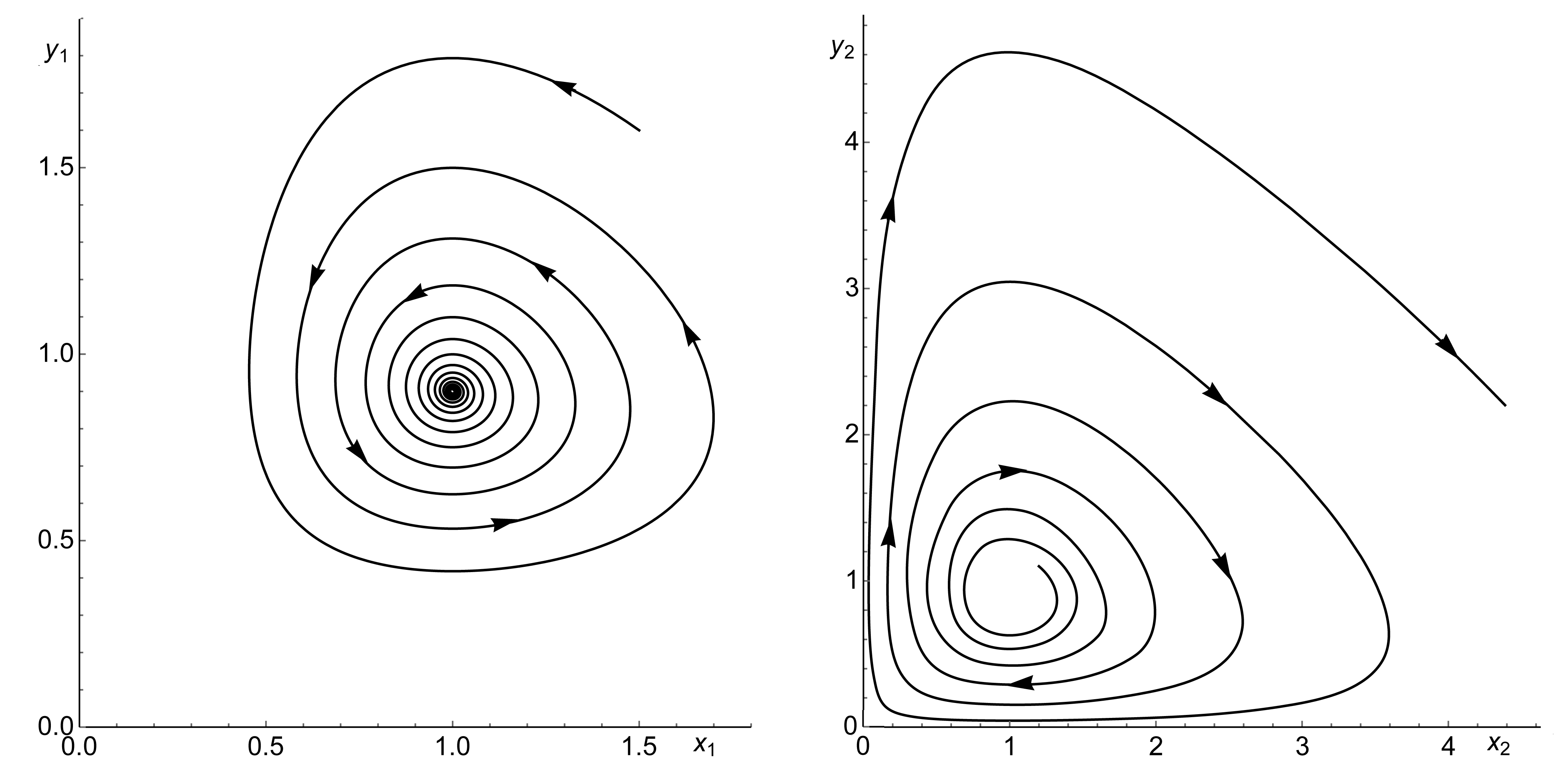
Figure 1: Left panel: An inspiral trajectory plotted in the $(x_{1},y_{1})$ plane for the dynamical subsystem (4) with $c=0.1$. The initial conditions are $x_{1}(0)=1.5,~{}y_{1}(0)=1.6$. Right panel: An outspiral trajectory for (5) in the $(x_{2},y_{2})$ plane with $c=0.1$. The initial conditions are $x_{2}(0)=1.2,~{}y_{2}(0)=1.1$. In the left panel $t$ ranges from $0$ to $100$ and in the right panel $t$ ranges from $0$ to $45$.

Next, we consider the $\mathcal{PT}$ reflection ($x_{1}\to x_{2}$, $y_{1}\to y_{2}$, $t\to-t$) of the subsystem in (4):

$$\dot{x}_{2} = -x_{2}+x_{2}y_{2}+cx_{2}^{2},$$

$$\dot{y}_{2} = y_{2}-x_{2}y_{2}.$$ (5)

The trajectories of this system are outspirals, as shown in Fig. 1 (right panel). The time evolution of the four dynamical variables in Fig. 1, $x_{1}(t)$ and $y_{1}(t)$, $x_{2}(t)$ and $y_{2}(t)$, is shown in Fig. 2.

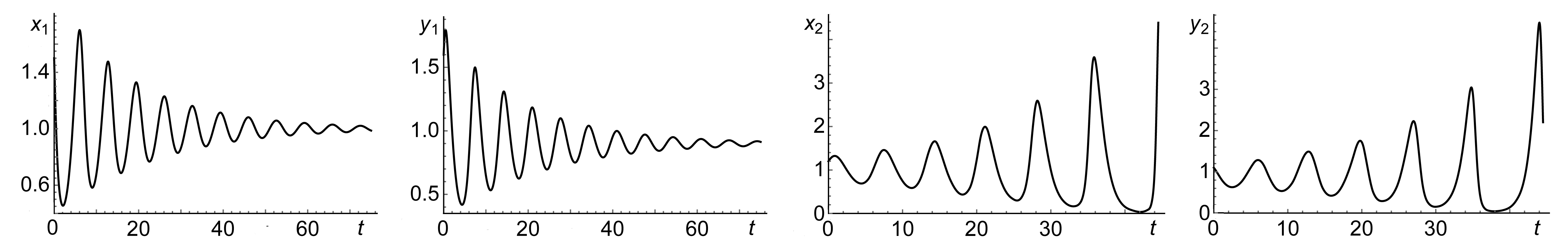
Figure 2: Inspiral and outspiral for the initial conditions in Fig. 1. The four variables $x_{1}(t)$, $y_{1}(t)$, $x_{2}(t)$, and $y_{2}(t)$ are plotted as functions of $t$.

Let us now couple the two subsystems in (4) and (5) in such a way that the $\mathcal{PT}$ symmetry is preserved. The resulting dynamical system obeys the nonlinear equations

$$\dot{x}_{1} = x_{1}-x_{1}y_{1}-cx_{1}^{2}+gx_{1}x_{2},$$

$$\dot{y}_{1} = -y_{1}+x_{1}y_{1}+fy_{1}y_{2},$$

$$\dot{x}_{2} = -x_{2}+x_{2}y_{2}+cx_{2}^{2}-gx_{1}x_{2},$$

$$\dot{y}_{2} = y_{2}-x_{2}y_{2}-fy_{1}y_{2}$$ (6)

in which $f$ and $g$ are the coupling parameters. This system has a wide range of possible behaviors. For example, for the parametric values $c=0.2$, $f=0.2$, and $g=0.5$ and the initial conditions $x_{1}(0)=y_{1}(0)=x_{2}(0)=y_{2}(0)=1.0$ we can see from Figs. 3 and 4 that the system is in a broken-$\mathcal{PT}$-symmetric phase.

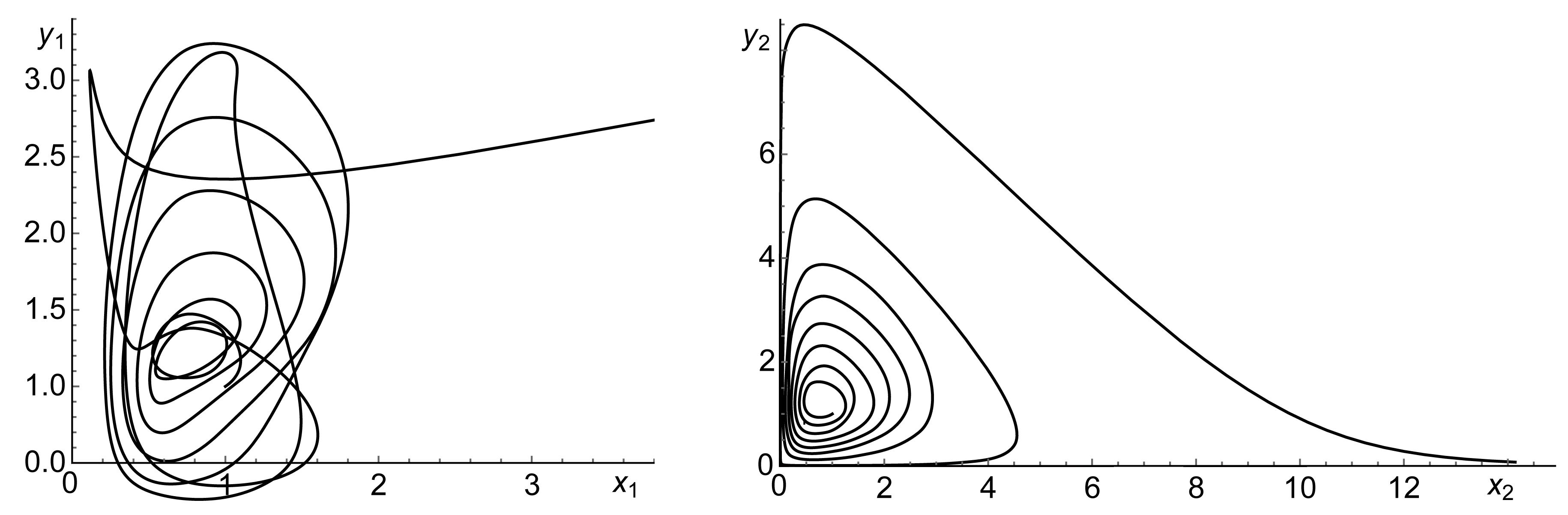
Figure 3: $\mathcal{PT}$-symmetric system (6) in a broken-$\mathcal{PT}$-symmetric phase, as indicated by the outspiral behavior in the $[x_{1}(t),y_{1}(t)]$ and $[x_{2}(t),y_{2}(t)]$ planes. The parametric values are $c=0.2$, $f=0.2$, and $g=0.5$ and the initial conditions are $x_{1}(0)=y_{1}(0)=x_{2}(0)=y_{2}(0)=1.0$. In these plots $t$ ranges from $0$ to $60$.

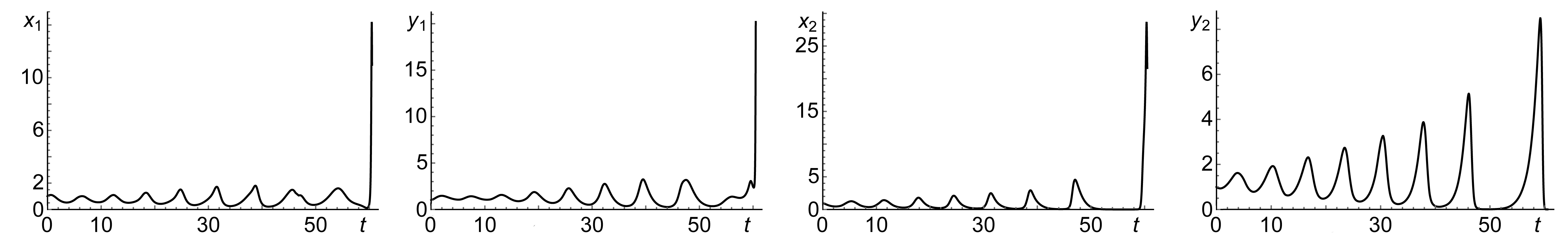
Figure 4: Time dependence of $x_{1}(t)$, $y_{1}(t)$, $x_{2}(t)$, $y_{2}(t)$ for the parametric values and initial conditions shown in Fig. 3.

When the coupling parameters are chosen so that the system (6) is in a phase of unbroken $\mathcal{PT}$ symmetry, the initial conditions determine whether the behavior is chaotic or almost periodic. For example, for the same parametric values $c=0.2$, $f=0.2$, and $g=0.3$ the system in (6) is in an unbroken-$\mathcal{PT}$-symmetric phase. Two qualitatively different behaviors of unbroken $\mathcal{PT}$ symmetry are illustrated in Figs. 5, 6, 7 and 8, 9, and 10. The first three figures display the system in two states of chaotic equilibrium and the next three show the system in two states of almost-periodic equilibrium. The Poincaré plots in Figs. 5 and 6 (left panels) and Figs. 8 and 9 (left panels) distinguish between chaotic and almost periodic behavior.

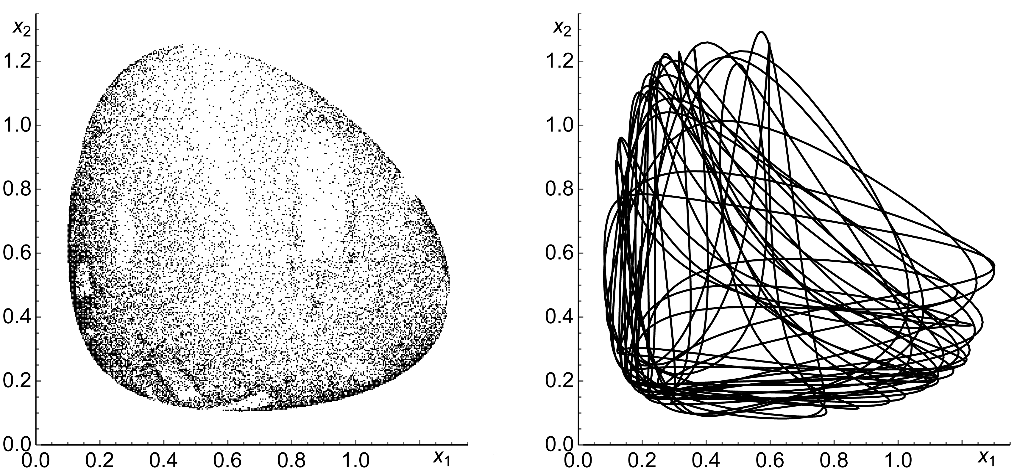
Figure 5: System (6) in a phase of chaotic unbroken $\mathcal{PT}$ symmetry. The parametric values are $c=0.2$, $f=0.5$, $g=0.3$ and the initial conditions are $x_{1}(0)=y_{1}(0)=x_{2}(0)=y_{2}(0)=0.5$. Left panel: Poincaré plot of $x_{1}$ versus $x_{2}$ when $y_{2}=0.75$. The two-dimensional scatter of dots indicates that the system is chaotic. In this plot $t$ ranges from $0$ to $100,000$. Right panel: A plot of $x_{1}(t)$ versus $x_{2}(t)$ for $t$ ranging from $0$ to $300$.

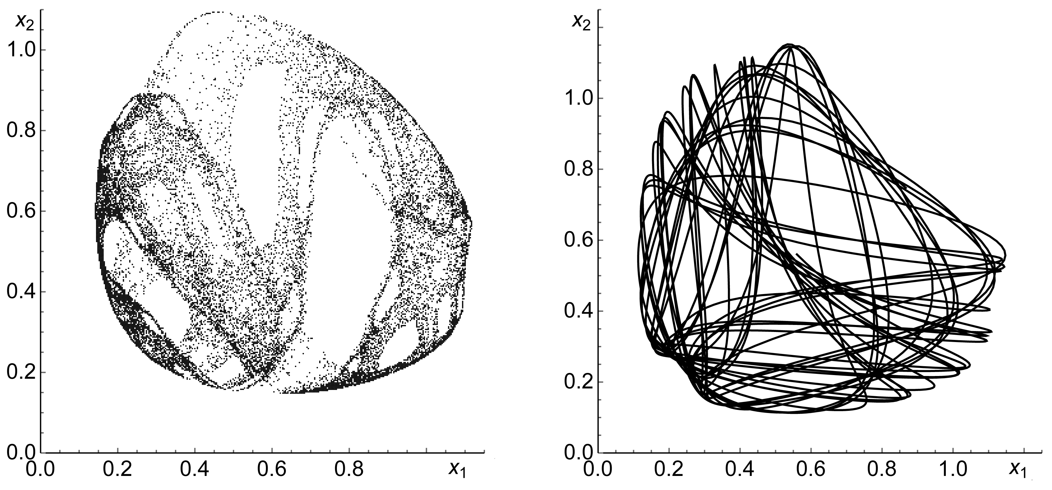
Figure 6: System in Fig. reff5 in a different chaotic state of unbroken $\mathcal{PT}$ symmetry. The parametric values and the ranges of $t$ are the same as in Fig. 5, but the initial conditions are now $x_{1}(0)=y_{1}(0)=x_{2}(0)=y_{2}(0)=0.56$.

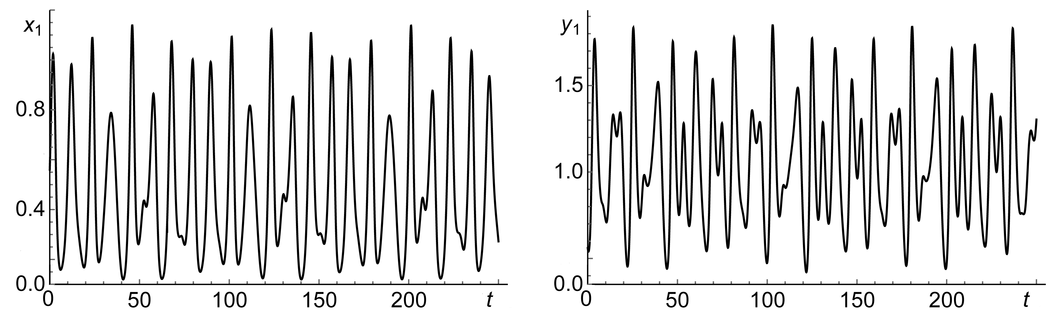
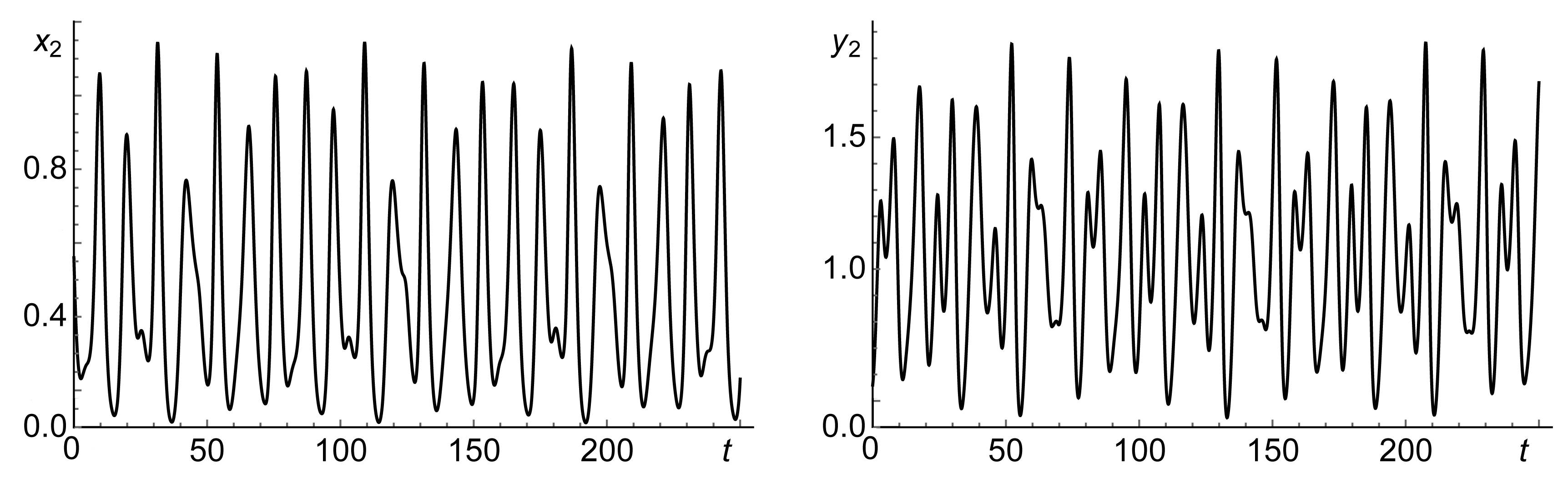
Figure 7: The system in Fig. 6 plotted as a function of time. The chaotic behavior can be seen as the uneven oscillations. These oscillations are reminiscent of a trajectory under the influence of a pair of strange attractors.

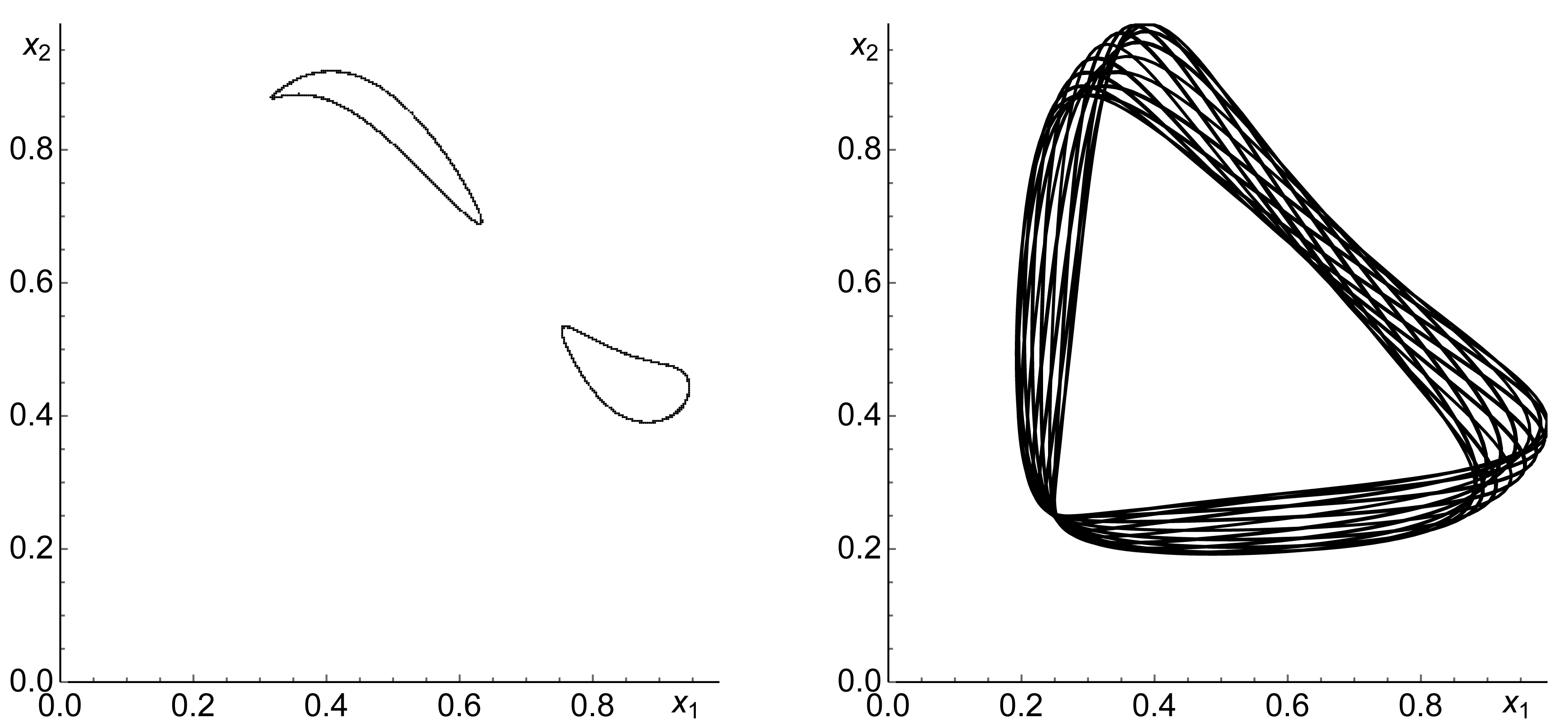
Figure 8: System (6) in a state of unbroken $\mathcal{PT}$ symmetry. The parametric values and the time ranges are the same as in Fig. 5, but the initial conditions are $x_{1}(0)=y_{1}(0)=x_{2}(0)=y_{2}(0)=0.68$. The presence of one-dimensional islands in the Poincaré plot (left panel) shows that the time evolution of the system is almost periodic.

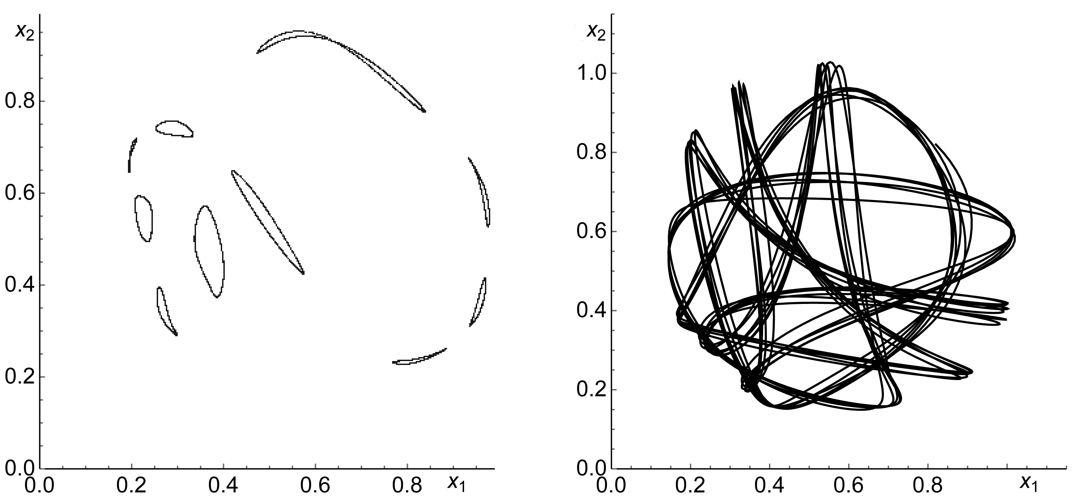
Figure 9: System (6) in a different state of unbroken $\mathcal{PT}$ symmetry. The parametric values and the ranges of $t$ are the same as in Fig. 8, but the initial conditions are $x_{1}(0)=y_{1}(0)=x_{2}(0)=y_{2}(0)=0.82$. The Poincaré plot (left panel) again shows that the time evolution of the system is almost periodic.

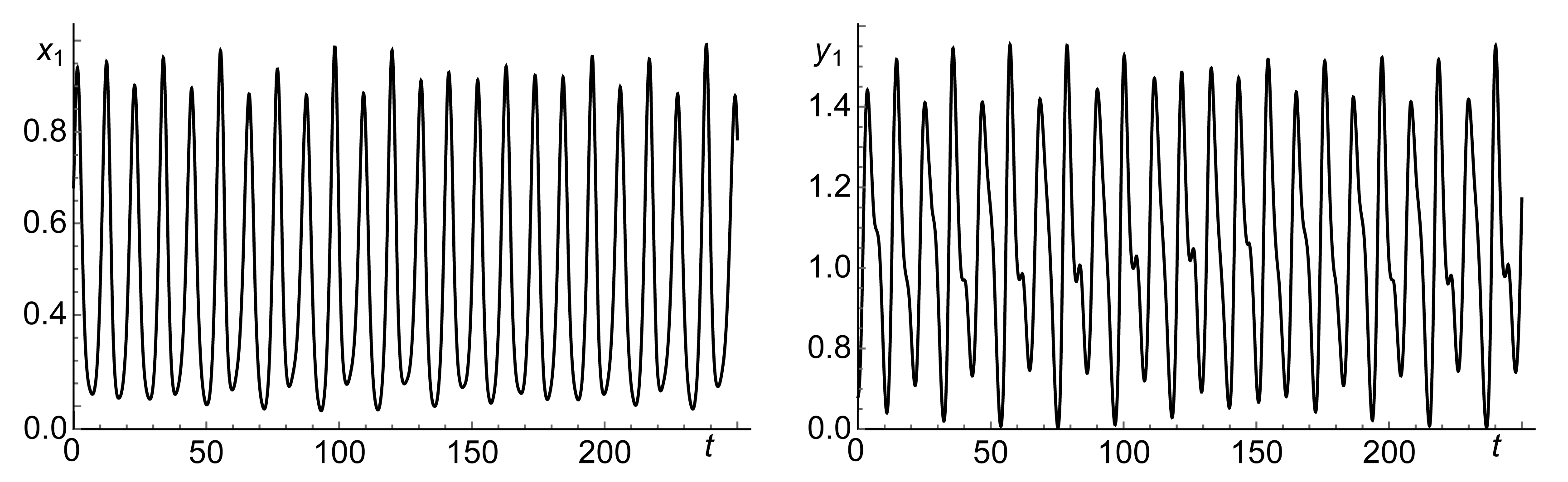
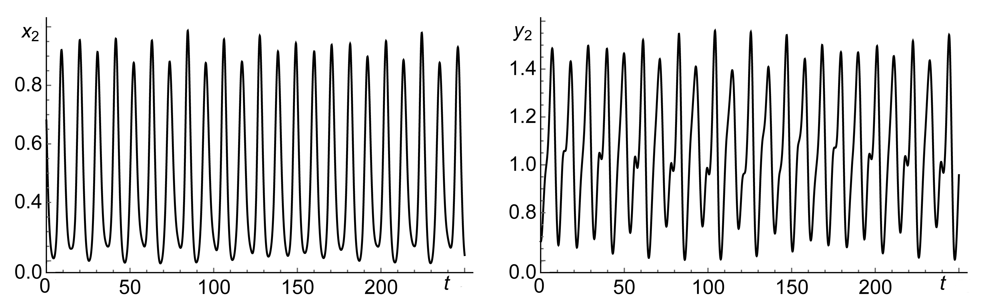
Figure 10: The system in Fig. 9 plotted as a function of time. The almost periodic behavior is particularly evident in the graphs on the left, where the oscillations are quite regular.

The choice of coupling parameters usually (but not always) determines whether the system is in an unbroken or a broken $\mathcal{PT}$-symmetric phase. To demonstrate this, we take $c=0.2$ and examine the time evolution for roughly 11,000 values of the parameters $f$ and $g$. Figure 11 indicates the values of $f$ and $g$ for which the system is in a broken or an unbroken (chaotic or almost periodic) phase.

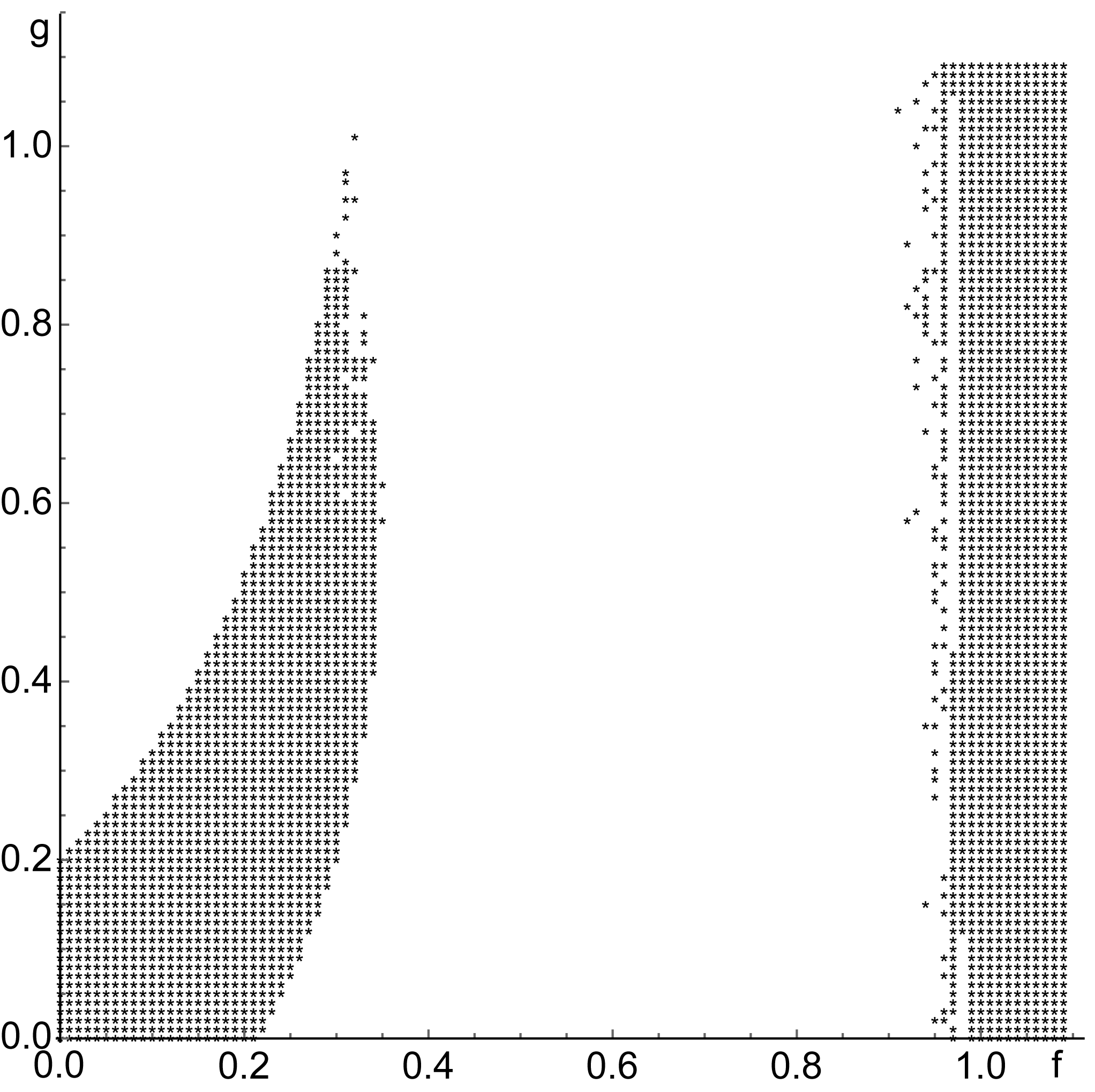
Figure 11: A region of the $(f,g)$ plane for the system (6) with the parametric value $c=0.2$. The initial conditions are $x_{1}(0)=y_{1}(0)=x_{2}(0)=y_{2}(0)=1$. The dots correspond to parametric values $(f,g)$ in the region of broken $\mathcal{PT}$ symmetry, and the white space corresponds to the region of unbroken $\mathcal{PT}$ symmetry. The edges of the regions are not completely sharp; it can be difficult to determine the precise location of the boundary curves separating broken and unbroken regions because this requires integrating for extremely long times.

Having summarized the possible behaviors of coupled $\mathcal{PT}$-symmetric dynamical subsystems, in Sec. II we construct and examine in detail a $\mathcal{PT}$-symmetric dynamical model of an antigen-antibody system containing two antigens and two antibodies. This system is similar in structure to that in (6). We show that in the unbroken region the concentrations of antigens and antibodies generally become chaotic and we interpret this as a chronic infection. However, in the unbroken regions there are two possibilities; either the antigen concentration grows out of bounds (the host dies) or else the antigen concentration falls to zero (the disease is completely cured). Some concluding remarks are given in Sec. III.

II Dynamical Model of Competing Antibody-Antigen Systems

Infecting an animal with bacteria, foreign cells, or virus may produce an immune response. The foreign material provoking the response is called an antigen and the immune response is characterized by the production of antibodies, which are molecules that bind specifically to the antigen and cause its destruction. The time-dependent immune response to a replicating antigen may be treated as a dynamical system with interacting populations of the antigen, the antibodies, and the cells that are involved in the production of antibodies. A detailed description of such an immune response would be extremely complicated so in this paper we consider a simplified mathematical model of the immune response proposed by Bell R1 . Bell’s paper introduces a simple model in which the multiplication of antigen and antibodies is assumed to be governed by Lokta-Volterra-type equations, where the antigen plays the role of prey and the antibody plays the role of predator. While such a model may be an unrealistic simulation of an actual immune response, Bell argues that this mathematical approach gives a useful qualitative and quantitative description.

Following Bell’s paper we take the variable $x_{1}(t)$ to represent the concentration of antibody and the variable $y_{1}(t)$ to represent the concentration of antigen at time $t$. Assuming that the system has an unlimited capability of antibody production, Bell’s dynamical model describes the time dependence of antigen and antibody concentrations by the differential equations

$$\dot{x}_{1} = -\lambda_{2}\,x_{1}+\alpha_{2}\,u(x_{1},y_{1}),$$

$$\dot{y}_{1} = \lambda_{1}\,y_{1}-\,\alpha_{1}\,v(x_{1},y_{1}).$$ (7)

According to (7), the antigen concentration $y_{1}$ increases at a constant rate $\lambda_{1}$ if the antibody $x_{1}$ is are not present. As soon as antigens are bound to antibodies, the antibodies start being eliminated at the constant rate $\alpha_{1}$. Analogously, the concentration of antibody $x_{1}$ decays with constant rate $\lambda_{2}$ in the absence of antigens, while binding of antigens to antibodies stimulates the production of antibody $x_{1}$ with constant rate $\alpha_{2}$. The functions $u(x_{1},y_{1})$ and $v(x_{1},y_{1})$ denote the concentrations of bound antibodies and bound antigens. Assuming that $u(x_{1},y_{1})=v(x_{1},y_{1})$, an approximate expression for the concentration of bound antigens and antibodies is

$$u(x_{1},y_{1})=v(x_{1},y_{1})=\frac{k\,x_{1}\,y_{1}}{1+k(x_{1}+y_{1})}\equiv F(x_{1},y_{1}),$$ (8)

where $k$ is called an association constant. With the scalings $kx_{1}\to x_{1}$ and $ky_{1}\to y_{1}$ and the change of variable

$$s=\int_{0}^{t}\,dt^{\prime}\,\left[1+x_{1}(t^{\prime})+y_{1}(t^{\prime})\right]^{-1},$$

system (7) becomes

$$\frac{dx_{1}}{ds} = -\lambda_{2}\,x-\lambda_{2}\,x_{1}^{2}+(\alpha_{2}-\lambda_{2})x_{1}y_{1},$$

$$\frac{dy_{1}}{ds} = \lambda_{1}\,y_{1}+\lambda_{1}\,y_{1}^{2}-(\alpha_{1}-\lambda_{1})x_{1}y_{1}.$$ (9)

The system (9) exhibits four different behaviors:

• If $R\equiv\alpha_{1}\alpha_{2}-\alpha_{1}\lambda_{2}-\alpha_{2}\lambda_{1}<0$, there is unbounded monotonic growth of antigen.

• If $R>0$ and $\alpha_{1}>\alpha_{2}$, there is an outspiral (oscillating growth of antigen).

• If $R>0$ and $\alpha_{1}<\alpha_{2}$, there is an inspiral (the antigen approaches a limiting value in an oscillatory fashion).

• If $R>0$ and $\alpha_{1}=\alpha_{2}$, the system exhibits exactly periodic oscillations. This behavior is unusual in a nonlinear system and indeed (6) does not exhibit exact periodic behavior.

II.1 $\mathcal{PT}$-symmetric interacting model

Subsequent to Bell’s paper R1 there have been many studies that use two-dimensional dynamical models to examine the antigen-antibody interaction RAA . However, in this paper we construct a four-dimensional model consisting of two antigens and two antibodies. Let us assume that an antigen $y_{1}$ attacks an organism and that the immune response consists of creating antibodies $x_{1}$ as described by (7). However, we suppose that the organism has a second system of antibodies and antigens $(x_{2},y_{2})$. This second subsystem plays the role of a $\mathcal{PT}$-symmetric partner of the system $(x_{1},y_{1})$, where parity $\mathcal{P}$ interchanges the antibody $x_{1}$ with the antigen $y_{2}$ and the antigen $y_{1}$ with the antibody $x_{1}$,

$$\mathcal{P}:\,x_{1}\to y_{2},\quad x_{2}\to y_{1},$$

and time reversal $\mathcal{T}$ makes the replacement $t\to-t$. The time evolution of this new antibody-antigen system is regulated by the equations

$$\dot{x}_{2} = -\lambda_{1}\,x_{2}+\alpha_{1}\,F(x_{2},y_{2}),$$

$$\dot{y}_{2} = \lambda_{2}\,y_{2}-\,\alpha_{2}\,F(x_{2},y_{2}).$$ (10)

We assume that the interaction between antibody $x_{2}$ and antigen $y_{2}$ is controlled by the same constant $k$ as in (8).

We assume that because antibodies may have many possible binding sites, $x_{1}$ can also bind to antigen $y_{2}$ and that antibody $x_{2}$ can also bind to antigen $y_{1}$. Moreover, for this model we assume that we can scale the dynamical variables so that this interaction is the same as the interaction $x_{1}-y_{1}$ and $x_{2}-y_{2}$. This means that after the scaling $kx_{1}\to x_{1}$, $ky_{1}\to y_{1}$, $kx_{2}\to x_{2}$, and $ky_{2}\to y_{2}$, the dynamical behavior of the total system $(x_{1},y_{1},x_{2},y_{2})$ is described by

$$\dot{x}_{1} = -\lambda_{2}x_{1}+\alpha_{2}\frac{x_{1}y_{1}}{1+x_{1}+y_{1}}+g\frac{x_{1}y_{2}}{1+x_{1}+y_{2}},$$

$$\dot{y}_{1} = \lambda_{1}y_{1}-\alpha_{1}\frac{x_{1}y_{1}}{1+x_{1}+y_{1}}-f\frac{x_{2}y_{1}}{1+x_{2}+y_{1}},$$

$$\dot{x}_{2} = -\lambda_{1}x_{2}+\alpha_{1}\frac{x_{2}y_{2}}{1+x_{2}+y_{2}}+f\frac{x_{2}y_{1}}{1+x_{2}+y_{1}},$$

$$\dot{y}_{2} = \lambda_{2}y_{2}-\alpha_{2}\frac{x_{2}y_{2}}{1+x_{2}+y_{2}}-g\frac{x_{1}y_{2}}{1+x_{1}+y_{2}}.$$ (11)

The production of the antibody $x_{2}$ is stimulated by the presence of the antigen $y_{2}$. The terms involving the parameter $f$ describe the production of additional antibodies $x_{2}$ and additional elimination of antigens $y_{1}$. Similarly, $g$ terms describe the production of new antibodies $x_{1}$ and additional elimination of antigens $y_{2}$.

II.2 Hamiltonian for (11)

We remark that the system (11) with $\alpha_{1}=\alpha_{2}=\alpha$ can be derived from the Hamiltonian R6

$$H=\alpha x^{-\lambda_{1}/\alpha}y^{-\lambda_{2}/\alpha}(1+x+y).$$ (12)

That is, it can be recovered from the Hamilton equations

$$\frac{\partial H}{\partial x}=J_{12}(x,y)\,\dot{y},\qquad\frac{\partial H}{\partial y}=J_{21}(x,y)\,\dot{x},$$ (13)

where

$$J_{21}(x,y)=-J_{12}(x,y)=x^{-1-\lambda_{1}/\alpha}\,y^{-1-\lambda_{2}/\alpha}.$$

II.3 Numerical results

Figure 12 displays a phase diagram of the $\mathcal{PT}$-symmetric model in (11), where we have taken $\lambda_{1}=\lambda_{2}=0.1$, $\alpha_{1}=0.6$, and $\alpha_{2}=0.5$. In this figure a portion of the $(f,g)$ plane is shown and the regions of broken and unbroken $\mathcal{PT}$ symmetry are indicated. Unbroken-$\mathcal{PT}$-symmetric regions are indicated as hyphens (blue online). There are two kinds of broken-$\mathcal{PT}$-symmetric regions; x’s (red online) indicate solutions that grow out of bounds and o’s (green online) indicate solutions for which the concentration of antigen $y_{1}$ approaches 0.

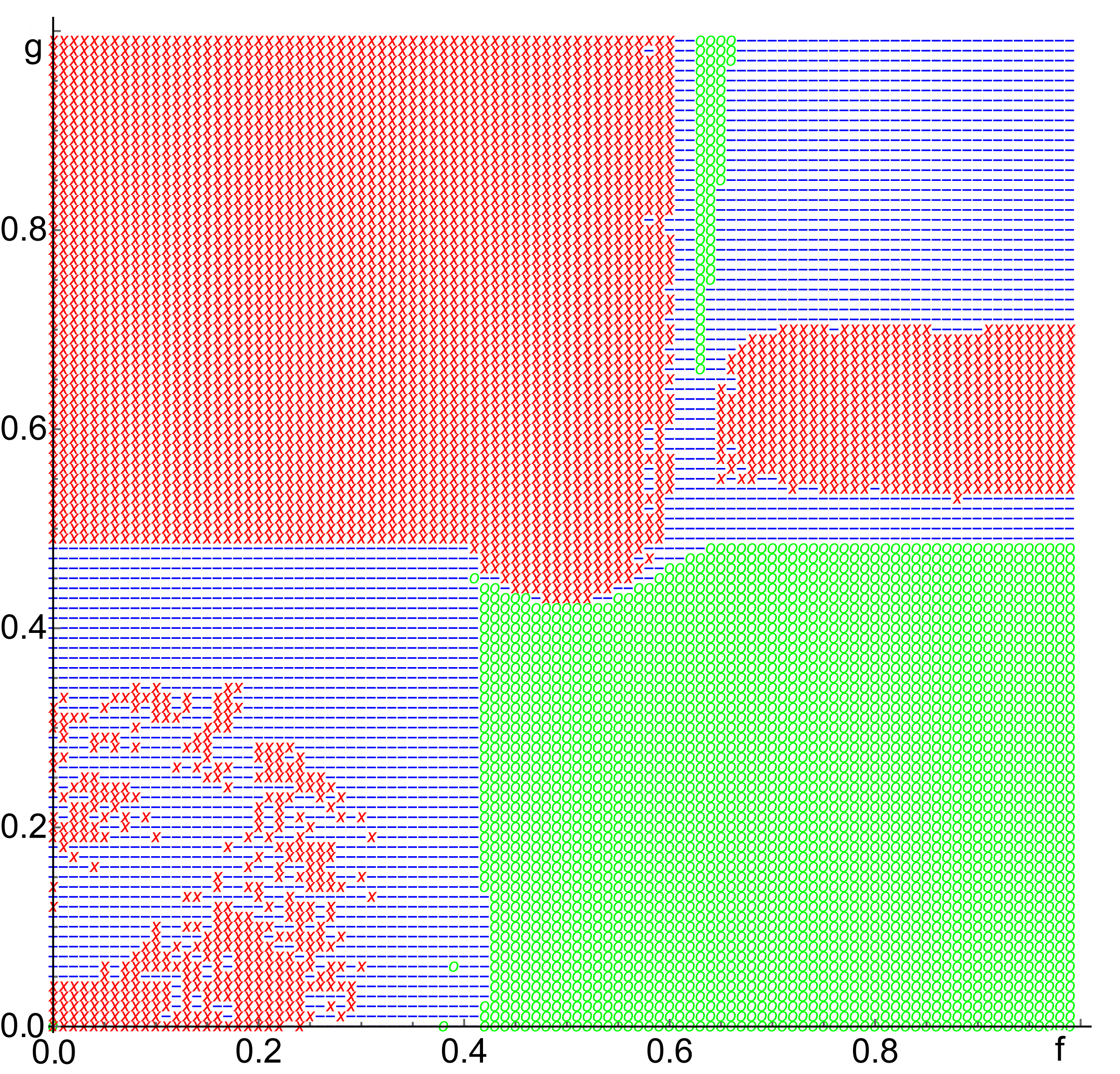
Figure 12: [Color online] Portion of the $(f,g)$ coupling-parameter plane for the $\mathcal{PT}$-symmetric immune-response system (11) showing regions of broken and unbroken $\mathcal{PT}$ symmetry. We take as initial conditions $x_{1}(0)=y_{1}(0)=1$ and $x_{2}(0)=x_{2}(0)=0.01$; that is, we assume that the disease associated with antigen-antibody 1 is well established and that at $t=0$ a very small amount of antigen-antibody 2 is injected. Points in the unbroken region are indicated as hyphens (blue). In this region the concentrations $x_{1},y_{1},x_{2},y_{2}$ are all oscillatory in time. In general, depending on the initial conditions, the solutions can be either almost periodic or chaotic. However, as shown in Fig. 16, the solutions to (11) are chaotic. Thus, in this region the introduction of antigen-antibody 2 makes the potentially lethal infection chronic. The regions whose points are indicated as o’s (green) and x’s (red) have broken $\mathcal{PT}$ symmetry. In the x regions the solutions oscillate and grow out of bounds. In the o regions $x_{1}(t)$ and $y_{1}(t)$ vanish and $x_{2}(t)$ and $y_{2}(t)$ approach small finite values as $t\to\infty$. Thus, in the x regions the host dies, but in the o regions the disease due to antigen $y_{1}$ is completely cured.

Figure 13 shows that the organism does not survive if the second antibody-antigen pair $x_{2},y_{2}$ is not initially present. In this figure we take $x_{1}(0)=y_{1}(0)=1$ but we we take $x_{2}(0)=y_{2}(0)=0$.

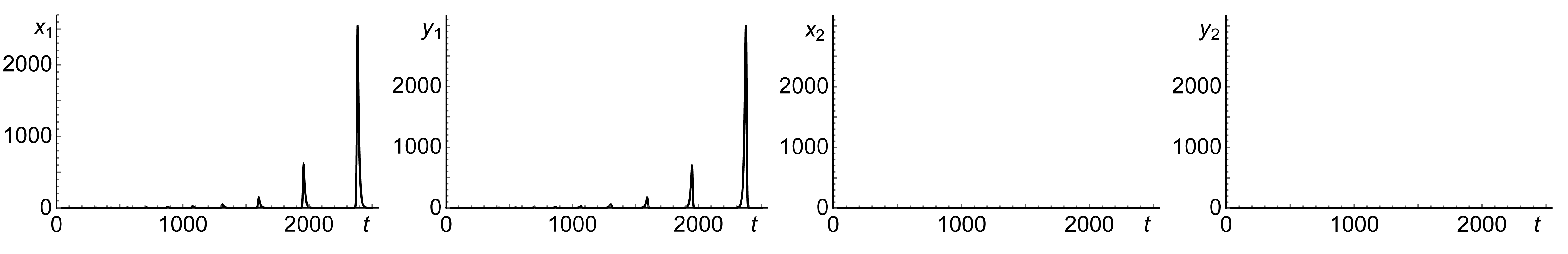
Figure 13: An organism that does not survive an antigen attack. Here, the antigen-antibody dynamics in (11) is described by (7) because we take $x_{2}(0)=y_{2}(0)=0$ and thus $x_{2}(t)$ and $y_{2}(t)$ remain 0 for all $t$. We have taken $\lambda_{1}=\lambda_{2}=0.1$, $\alpha_{1}=0.6$, and $\alpha_{2}=0.5$. The initial conditions are $x_{1}(0)=y_{1}(0)=1$.

Figure 14 shows what happens in a broken-$\mathcal{PT}$-symmetric phase when the organism does not survive. We take $f=0.02$ and $g=0.01$, which puts us in the lower-left corner of Fig. 12. The initial conditions are $x_{1}(0)=y_{1}(0)=1$ and $x_{2}(0)=y_{2}(0)=0.01$. Note that the level of the $y_{1}(t)$ antigen grows out of bounds.

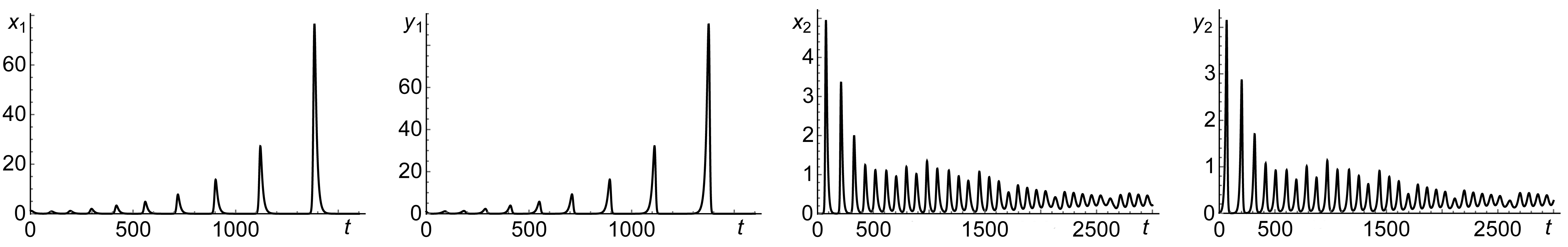
Figure 14: Antibody-antigen competition in the broken-$\mathcal{PT}$-symmetric phase in the lower-left corner of Fig. 12; specifically $f=0.02$ and $g=0.01$. The organism does not survive the antigen attack. The antigen-antibody dynamics is described by (11), where $\lambda_{1}$, $\lambda_{2}$, $\alpha_{1}$, $\alpha_{2}$, and the initial conditions are the same as in Fig. 12.

Figure 15 shows what happens in the unbroken region in Fig. 12. The organism survives but the disease becomes chaotically chronic.

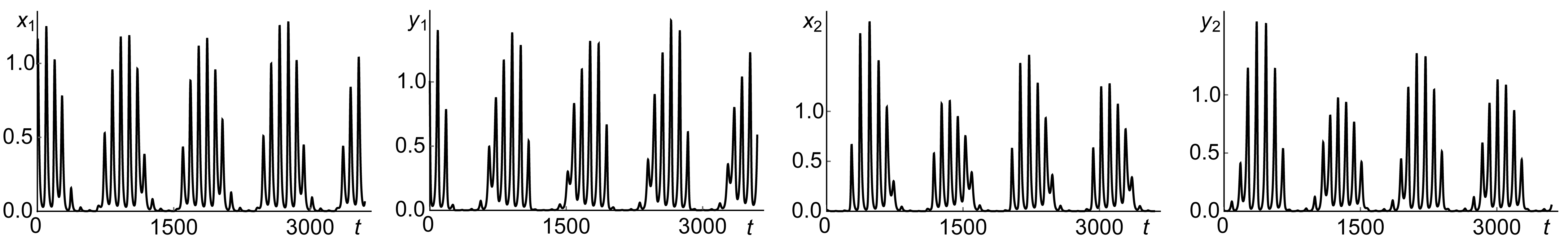
Figure 15: An organism that survives an antigen attack. The coupling parameters are chosen to be $f=0.32$ and $g=0.4$, which is in the unbroken-$\mathcal{PT}$ phase in the lower-left portion of Fig. 12. The antigen-antibody dynamics is described by (11), where $\lambda_{1}$, $\lambda_{2}$, $\alpha_{1}$, $\alpha_{2}$, and the initial conditions are the same as in Fig. 12. The concentrations of antigens and antibodies behave chaotically in time.

Figure 16 demonstrates the chaotic behavior at a point in the upper-right unbroken-$\mathcal{PT}$ portion of Fig. 12, specifically at $f=0.76$ and $g=0.80$. The figure shows a Poincaré map in the $(x_{1},y_{1})$ plane for $y_{2}=0.5$.

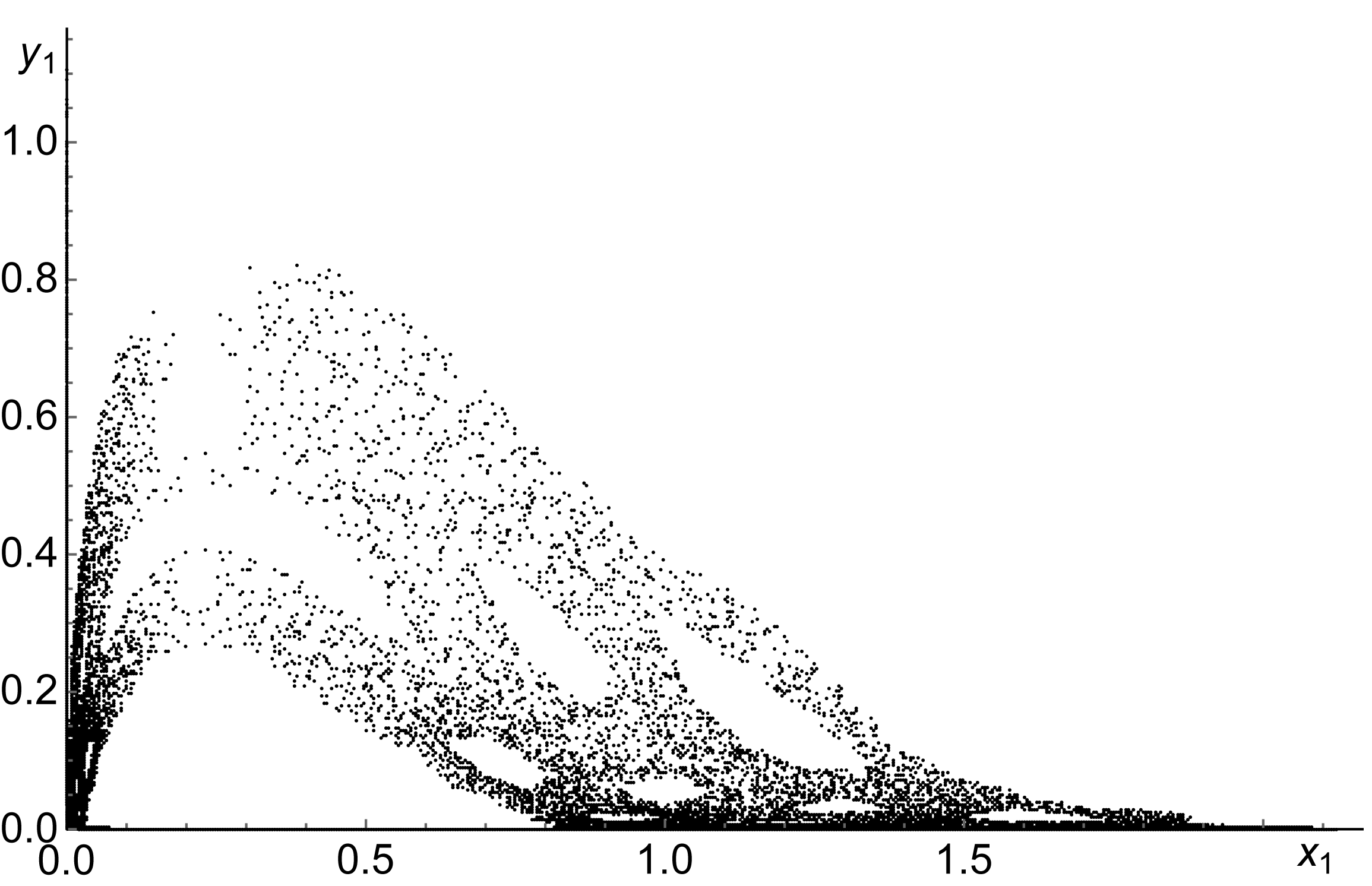
Figure 16: An organism that survives an antigen attack. The antigen-antibody dynamics is described by (11), where $\lambda_{1}$, $\lambda_{2}$, $\alpha_{1}$, $\alpha_{2}$, and the initial conditions are the same as in Fig. 12. In this plot $f=0.76$ and $g=0.80$, which places the system in the unbroken phase in the upper-right corner of Fig. 12. The dynamical behavior is chaotic and the disease becomes chronic, as implied by the Poincaré map in which trajectory points are plotted in the $(x_{1},y_{1})$ plane for $y_{2}=0.5$. The scatter of points indicates chaotic behavior. The time interval for the plot is from $t=0$ to $t=5,000,000$.

Figure 17 shows what happens in the broken-$\mathcal{PT}$ region in the lower-right corner of Fig. 12 at $f=0.5$ and $g=0.2$. In this region the antigen $y_{1}(t)$ completely disappears and the disease is cured.

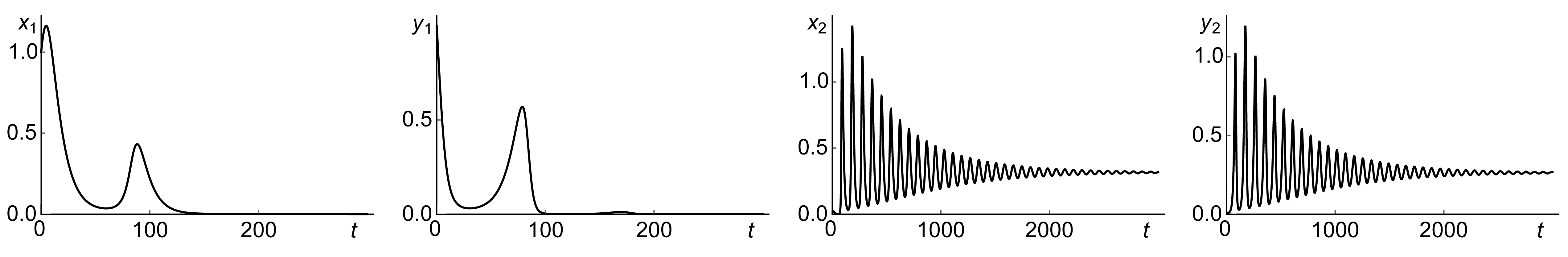
Figure 17: An organism that survives an antigen attack. This figure shows what happens at the point $f=0.5$ and $g=0.2$ in the broken-$\mathcal{PT}$ region in the lower-right corner of Fig. 12. In this plot $\lambda_{1}$, $\lambda_{2}$, $\alpha_{1}$, $\alpha_{2}$, and the initial conditions are the same as in Fig. 12. Note that the antigen concentration $y_{1}(t)$ decays to zero and the disease is cured. The concentration of antigen $y_{2}$ approaches a small nonzero value as $t\to\infty$ and, as was noted in Ref. R1 , this value is so small that we regard it as negligible.

III Concluding remarks

In this paper we have extended Bell’s two-dimensional predator-prey model of an immune response to a four-dimensional $\mathcal{PT}$-symmetric model and have examined the outcomes in the broken- and the unbroken-$\mathcal{PT}$-symmetric phases. We have found that in the unbroken phase the disease becomes chronic (oscillating) while in the broken phase the host may die or be completely cured.

In Bell’s model (Ref. R1 ) an oscillating regime is assumed to be a transitory state and that either the antigen is completely eliminated at an antigen minimum or the host dies at an antigen maximum. However, there are many examples in which the immune system undergoes temporal oscillations (occurring in pathogen load in populations of specific cell types, or in concentrations of signaling molecules such as cytokines). Some well known examples are the periodic recurrence of a malaria infection R7 , familial Mediterranean fever R8 , or cyclic neutropenia R9 . It is not understood whether these oscillations represent some kind of pathology or if they are part of the normal functioning of the immune system, so they are generally regarded as aberrations and are largely ignored. A discussion of immune system oscillation can be found in Ref. R10 . Additional chaotic oscillatory diseases such as chronic salmonella, hepatitis B, herpes simplex, and autoimmune diseases such as multiple sclerosis, Crohn’s disease, and fibrosarcoma are discussed in Ref. R11 .

In Ref. R1 it is not possible to completely eliminate the antigen, that is, to make the antigen concentration go to zero. However, it is possible to reduce the antigen concentration to a very low level, perhaps corresponding to less than one antigen unit per host, which one can interpret as complete elimination. However, we will see that in the $\mathcal{PT}$-symmetric model (11) the antigen $x_{1}$ can actually approach 0 in the $\mathcal{PT}$ broken phase.

In Ref. R1 it is stated that the predicted oscillations of increasing amplitude should be viewed with caution. Such oscillations are predicted to involve successively lower antibody minima, which in reality may not occur. However, in Ref. R12 a modified two-dimensional predator-prey model for the dynamics of lymphocytes and tumor cells is considered. This model seems to reproduce all known states for a tumor. For certain parameters the system evolves towards a state of uncontrollable tumor growth and exhibits the same time evolution as that of $x_{1}$ and $y_{1}$ in Figs. 13 and 14. For other parameters the system evolves in an oscillatory fashion towards a controllable mass (a time-independent limit) of malignant cells. In this case the temporal evolution is the same as that of $x_{2}$ and $y_{2}$ in Fig. 17. In Ref. R12 this state is called a dormant state. It is also worth mentioning that in Ref. R13 a two-dimensional dynamical system describing the immune response to a virus is considered; this model can exhibit periodic solutions, solutions that converge to a fixed point, and solutions that have chaotic oscillations. Ordinarily, a two-dimensional dynamical system cannot have chaotic trajectories but the novelty in this system is that there is a time delay.

Finally, we acknowledge that it is not easy to select reasonable parameters if one considers the application of Bell’s model to real biological systems. In the $\mathcal{PT}$-symmetric model it is also difficult to make realistic estimates of relevant parameters. Nevertheless, we believe that some of the qualitative features described in this paper may also be seen in actual biological systems.

- (1) G. I. Bell, Math. Biosci. 16, 291 (1973).
- (2) C. M. Bender, Rept. Prog. Phys. 70, 947-1018 (2007).
- (3) C. M. Bender, M. Gianfreda, B. Peng, S. K. Ozdemir, and L. Yang, Phys. Rev. A 88, 062111 (2013).
- (4) B. Peng, S. K. Ozdemir, F. Lei, F. Monifi, M. Gianfreda, G. L. Long, S. Fan, F. Nori, C. M. Bender, L. Yang, Nat. Phys. 10, 394 (2014).
- (5) C. M. Bender, M. Gianfreda, and S. P. Klevansky, Phys. Rev. A 90, 022114 (2014).
- (6) J. Rubinstein, P. Sternberg, and Q. Ma, Phys. Rev. Lett. 99, 167003 (2007).
- (7) A. Guo, G. J. Salamo, D. Duchesne, R. Morandotti, M. Volatier-Ravat, V. Aimez, G. A. Siviloglou, and D. N. Christodoulides, Phys. Rev. Lett. 103, 093902 (2009).
- (8) C. E. Rüter, K. G. Makris, R. El-Ganainy, D. N. Christodoulides, M. Segev, and D. Kip, Nat. Phys. 6, 192-195 (2010).
- (9) K. F. Zhao, M. Schaden, and Z. Wu, Phys. Rev. A 81, 042903 (2010).
- (10) Z. Lin, H. Ramezani, T. Eichelkraut, T. Kottos, H. Cao, and D. N. Christodoulides, Phys. Rev. Lett. 106, 213901 (2011).
- (11) L. Feng, M. Ayache, J. Huang, Y.-L. Xu, M. H. Lu, Y. F. Chen, Y. Fainman, and A. Scherer, Science 333, 729 (2011).
- (12) S. Bittner, B. Dietz, U. Günther, H. L. Harney, M. Miski-Oglu, A. Richter, and F. Schäfer, Phys. Rev. Lett. 108, 024101 (2012).
- (13) N. Chtchelkatchev, A. Golubov, T. Baturina, and V. Vinokur, Phys. Rev. Lett. 109, 150405 (2012).
- (14) C. Zheng, L. Hao, and G. L. Long, Phil. Trans. R. Soc. A 371, 20120053 (2013).
- (15) J. Schindler, A. Li, M. C. Zheng, F. M. Ellis, and T. Kottos, Phys. Rev. A 84, 040101(R) (2011).
- (16) C. M. Bender, D. D. Holm, and D. W. Hook, J. Physics A: Math. Theor. 40, F793 (2007).
- (17) I. V. Barashenkov and M. Gianfreda, J. Phys. A: Math. Theor. 47, 282001(FTC) (2014).
- (18) A. S. Perelson and G. Weisbuch, Rev. Mod. Phys. 69,1219 (1997).
- (19) M. Plank, J. Math. Phys. 36, 7 (1995).
- (20) R. S. Desowitz, The Malaria Capers: More Tales of Parasites and People, Research and Reality (Norton, New York, 1991); C. M. Poser and G. W. Bruyn, An Illustrated History of Malaria (Parthenon, New York, 1999).
- (21) J. P. H. Drenth, Hyper-IgD syndrome, a life with fever, PhD Thesis, Nijmegen, (1996).
- (22) D. C. Dale and W. P. T. Hammond, Blood Rev. 2, 178 (1988).
- (23) J. Stark, C. Chan, and A. J. T. George, Immunological Review 216 213, (2007).
- (24) H. Mayer, K. S. Zaenker, and U. an der Heiden, Chaos 5, 155 (1995).
- (25) O. Sotolongo-Costa, L. Morales Molina, D. Rodrígues Perez, J. C. Antoranz, M. Chacón Reyes, Physica D 78, 242 (2003).
- (26) H. Shu, L. Wang and J. Watmough J. Math. Biol. 68, 477 (2014).