Optimal Monotone Drawings of Trees

Abstract

A monotone drawing of a graph $G$ is a straight-line drawing of $G$ such that, for every pair of vertices $u,w$ in $G$, there exists a path $P_{uw}$ in $G$ that is monotone in some direction $l_{uw}$. (Namely, the order of the orthogonal projections of the vertices of $P_{uw}$ on $l_{uw}$ is the same as the order they appear in $P_{uw}$.)

The problem of finding monotone drawings for trees has been studied in several recent papers. The main focus is to reduce the size of the drawing. Currently, the smallest drawing size is $O(n^{1.205})\times O(n^{1.205})$. In this paper, we present an algorithm for constructing monotone drawings of trees on a grid of size at most $12n\times 12n$. The smaller drawing size is achieved by a new simple Path Draw algorithm, and a procedure that carefully assigns primitive vectors to the paths of the input tree $T$.

We also show that there exists a tree $T_{0}$ such that any monotone drawing of $T_{0}$ must use a grid of size $\Omega(n)\times\Omega(n)$. So the size of our monotone drawing of trees is asymptotically optimal.

1 Introduction

A straight-line drawing of a plane graph $G$ is a drawing $\Gamma$ in which each vertex of $G$ is drawn as a distinct point on the plane and each edge of $G$ is drawn as a line segment connecting two end vertices without any edge crossing. A path $P$ in a straight-line drawing $\Gamma$ is monotone if there exists a line $l$ such that the orthogonal projections of the vertices of $P$ on $l$ appear along $l$ in the order they appear in $P$. We call $l$ a monotone line (or monotone direction) of $P$. $\Gamma$ is called a monotone drawing of $G$ if it contains at least one monotone path $P_{uw}$ between every pair of vertices $u,w$ of $G$. We call the monotone direction $l_{uw}$ of $P_{uw}$ the monotone direction for $u,w$.

Monotone drawing introduced by Angelini et al. [1] is a new visualization paradigm. Consider the example described in [1]: a traveler uses a road map to find a route from a town $u$ to a town $w$. He would like to easily spot a path connecting $u$ and $w$. This task is harder if each path from $u$ to $w$ on the map has legs moving away from $u$. The traveler rotates the map to better perceive its content. Hence, even if in the original map orientation all paths from $u$ to $w$ have annoying back and forth legs, the traveler might be happy to find one map orientation where a path from $u$ to $w$ smoothly goes from left to right. This approach is also motivated by human subject experiments: it was shown that the “geodesic tendency” (paths following a given direction) is important in understanding the structure of the underlying graphs [12].

Monotone Drawing is also closely related to several other important graph drawing problems. In a monotone drawing, each monotone path is monotone with respect to a different line. In an upward drawing [6, 7], every directed path is monotone with respect to the positive $y$ direction. Even more related to the monotone drawings are the greedy drawings [2, 14, 16]. In a greedy drawing, for any two vertices $u,v$, there exists a path $P_{uv}$ from $u$ to $v$ such that the Euclidean distance from an intermediate vertex of $P_{uv}$ to the destination $v$ decreases at each step. Nöllenburg et al. [15] observed that while getting closer to the destination, a greedy path can make numerous turns and may even look like a spiral, which hardly matches the intuitive notion of geodesic-path tendency. In contrast, in a monotone drawing, there exists a path $P_{uv}$ from $u$ to $v$ (for any two vertices $u,v$) and a line $l_{uv}$ such that the Euclidean distance from the projection of an intermediate vertex of $P_{uv}$ on $l$ to the projection of the destination $v$ on $l$ decreases at each step. So the monotone drawing better captures the notion of geodesic-path tendency.

Related works: Angelini et al. [1] showed that every tree of $n$ vertices has a monotone drawing of size $O(n^{2})\times O(n)$ (using a DFS-based algorithm), or $O(n^{\log_{2}3})\times O(n^{\log_{2}3})=O(n^{1.58})\times O(n^{1.58})$ (using a BFS-based algorithm). It was also shown that every biconnected planar graph of $n$ vertices has a monotone drawing in real coordinate space. Several papers have been published since then. The focus of the research is to identify the graph classes having monotone drawings and, if so, to find monotone drawings for them with size as small as possible. Angelini (with another set of authors) [3] showed that every planar graph has a monotone drawing of size $O(n)\times O(n^{2})$. However, their drawing is not straight line. It may need up to $4n-10$ bends in the drawing. Recently Hossain and Rahman [11] showed that every planar graph has a monotone drawing. X. He and D. He [10] showed that the classical Schnyder drawing of 3-connected plane graphs on an $O(n)\times O(n)$ grid is monotone.

The monotone drawing problem for trees is particularly important. Any drawing result for trees can be applied to any connected graph $G$: First, we construct a spanning tree $T$ for $G$, then find a monotone drawing $\Gamma$ for $T$. $\Gamma$ is automatically a monotone drawing for $G$ (although not necessarily planar).

Both the DFS- and BFS-based tree drawing algorithms in previous papers use the so-called Stern-Brocot tree to generate a set of $n-1$ primitive vectors (will be defined later) in increasing order of slope. Then both algorithms do a post-order traversal of the input tree, assign each edge $e$ a primitive vector, and draw $e$ by using the assigned vector. Such drawings of trees are called slope-disjoint. Kindermann et al. [13] proposed another version of the slope-disjoint algorithm, but using a different set of primitive vectors (based on Farey sequence), which slightly decreases the grid size to $O(n^{1.5})\times O(n^{1.5})$. Recently, X. He and D. He reduced the drawing size to $O(n^{1.205})\times O(n^{1.205})$ by using a set of more compact primitive vectors [9].

A stronger version of monotone drawings is the strong monotone drawing: For every two vertices $u,w$ in the drawing of $G$, there must exist a path $P_{uw}$ that is monotone with respect to the line passing through $u$ and $w$. Since the strong monotone drawing is not a subject of this paper, we refer readers to [15] for related results and references.

Our results: We show that every $n$-vertex tree $T$ admits a monotone drawing on a grid of size $12n\times 12n$, which is asymptotically optimal.

The paper is organized as follows. Section 2 introduces definitions and preliminary results on monotone drawings. In Section 3, we give our algorithm for constructing monotone drawings of trees on a $12n\times 12n$ grid. In Section 4, we describe a tree $T_{0}$ and show that any monotone drawing of $T_{0}$ must use a grid of size $\Omega(n)\times\Omega(n)$. Section 5 concludes the paper and discusses some open problems.

2 Preliminaries

Let $p$ be a point in the plane and $l$ be a half-line with $p$ as its starting point. The angle of $l$, denoted by $\operatorname{angle}(l)$ is the angle spanned by a ccw (we abbreviate the word “counterclockwise” as ccw) rotation that brings the direction of the positive $x$-axis to overlap with $l$. We consider angles that are equivalent modulo $360^{\circ}$ as the same angle (e.g., $270^{\circ}$ and $-90^{\circ}$ are regarded as the same angle).

In this paper, we only consider straight line drawings (i.e., each edge of $G$ is drawn as a straight line segment between its end vertices.) Let $\Gamma$ be such a drawing of $G$ and let $e=(u,w)$ be an edge of $G$. The direction of $e$, denoted by $d(u,w)$ or $d(e)$, is the half-line starting at $u$ and passing through $w$. The angle of an edge $(u,w)$, denoted by $\operatorname{angle}(u,w)$, is the angle of $d(u,w)$. Observe that $\operatorname{angle}(u,w)=\operatorname{angle}(w,u)-180^{\circ}$. When comparing directions and their angles, we assume that they are applied at the origin of the axes.

Let $P(u_{1},u_{k})=(u_{1},\ldots,u_{k})$ be a path of $G$. We also use $P(u_{1},u_{k})$ to denote the drawing of the path in $\Gamma$. $P(u_{1},u_{k})$ is monotone with respect to a direction $l$ if the orthogonal projections of the vertices $u_{1},\ldots,u_{k}$ on $l$ appear in the same order as they appear along the path. $P(u_{1},u_{k})$ is monotone if it is monotone with respect to some direction. A drawing $\Gamma$ is monotone if there exists a monotone path $P(u,w)$ for every pair of vertices $u,w$ in $G$.

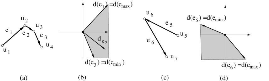
Figure 1: (a) A monotone path $P(u_{1},u_{4})$ with extremal edges $e_{1}$ and $e_{3}$; (b) The range of $P(u_{1},u_{4})$ defined by $d(e_{3})=d(e_{\min})$ and $d(e_{1})=d(e_{\max})$; (c) A monotone path $P(u_{5},u_{7})$ with only two edges $e_{5}$ and $e_{6}$; (d) The range of $P(u_{5},u_{7})$ defined by $d(e_{5})=d(e_{\min})$ and $d(e_{6})=d(e_{\max})$.

The following property is well-known [1]:

Property 1

A path $P(u_{1},u_{k})$ is monotone if and only if it contains two edges $e_{1}$ and $e_{2}$ such that the closed wedge centered at the origin of the axes, delimited by the two half-lines $d(e_{1})$ and $d(e_{2})$, and having an angle strictly smaller than $180^{\circ}$, contains all half-lines $d(u_{i},u_{i+1})$, for $i=1,\ldots,k-1$.

The two edges $e_{1}$ and $e_{2}$ in Property 1 are called the two extremal edges of $P(u_{1},u_{k})$, and the closed wedge (centered at the origin of the axes) delimited by the two half-lines $d(e_{1})$ and $d(e_{2})$, containing all the half-lines $d(u_{i},u_{i+1})$ for $i=1,\ldots,k-1$, is called the range of $P(u_{1},u_{k})$ and denoted by $\operatorname{range}(P(u_{1},u_{k}))$. See Fig 1 (a) and (b). We use $e_{\min}$ and $e_{\max}$ to denote the extremal edges $e_{1}$ and $e_{2}$ so that the wedge $\operatorname{range}(P(u_{1},u_{k}))$ is the area spanned by a ccw rotation that brings the half-line $d(e_{\min})$ to overlap with the half-line $d(e_{\max})$. Thus we have $\operatorname{angle}(e_{\min})<\operatorname{angle}(e_{\max})$. Note that, for a path with only two edges, we consider its range to be the closed wedge with an angle $\leq 180^{\circ}$. See Fig 1 (c) and (d).

The closed interval $[\operatorname{angle}(e_{\min}),\operatorname{angle}(e_{\max})]$ is called the scope of $P(u_{1},u_{k})$ and denoted by $\operatorname{scope}(P(u_{1},u_{k}))$. Note that $\operatorname{angle}(u_{i},u_{i+1})\in\operatorname{scope}(P(u_{1},u_{k}))$ for all edges $(u_{i},u_{i+1})$ ($i=1,\ldots,k-1$) in $P(u_{1},u_{k})$. By this definition, Property 1 can be restated as:

Property 2

A path $P(u_{1},u_{k})$ with scope $[\operatorname{angle}(e_{\min}),\operatorname{angle}(e_{\max})]$ is monotone if and only if $\operatorname{angle}(e_{\max})-\operatorname{angle}(e_{\min})<180^{\circ}$.

Define: $P_{d}=\{(x,y)~{}|~{}x\mbox{ and }y\mbox{ are integers, }\mbox{gcd}(x,y)=1,1\leq x\leq y\leq d\}$

If we consider each entry $(x,y)\in P_{d}$ to be the rational number $y/x$ and order them by value, we get the so-called Farey sequence ${\cal F}_{d}$ (see [8]). The property of the Farey sequence is well understood. It is known $|{\cal F}_{d}|=3d^{2}/\pi^{2}+O(d\log d)$ ([8], Thm 331). Thus, $|P_{d}|=|{\cal F}_{d}|\geq 3d^{2}/\pi^{2}$. Let $P^{\prime}_{d}$ be the set of the vectors that are the reflections of the vectors in $P_{d}$ through the line $x=y$. Define:

$$\overline{P_{d}}=P_{d}\cup P^{\prime}_{d}=\{(x,y)~{}|~{}x\mbox{ and }y\mbox{ are integers, }\mbox{gcd}(x,y)=1,1\leq x,y\leq d\}$$

The members of $\overline{P_{d}}$ are called the primitive vectors of size $d$. Fig 2 (a) shows the vectors in $\overline{P_{3}}$. We have $|\overline{P_{d}}|\geq 6d^{2}/\pi^{2}$. Moreover, the members of $\overline{P_{d}}$ can be enumerated in $O(|\overline{P_{d}}|)$ time [13]. Note that the vectors $(1,0)$ and $(0,1)$ are not vectors in $\overline{P_{d}}$. For easy reference, we call them the boundary vectors of $\overline{P_{d}}$.

Figure 2: (a) The vectors in $\overline{P_{3}}$; (b) a tree with edges ordered in ccw post-order; (c) the monotone drawing of the tree in (b) produced by Algorithm 1 by using vectors in (a); (d) the monotone drawing of the tree in (b) produced by Algorithm 2 by using vectors in (a).

Next, we outline the algorithm in [1] for monotone drawings of trees.

Definition 1

[1] A slope-disjoint drawing of a rooted tree $T$ is such that:

1. For each vertex $u$ in $T$, there exist two angles $\alpha_{1}(u)$ and $\alpha_{2}(u)$, with $0<\alpha_{1}(u)<\alpha_{2}(u)<180^{\circ}$ such that, for every edge $e$ that is either in $T(u)$ ($T(u)$ denotes the subtree of $T$ rooted at $u$) or that connects $u$ with its parent, it holds that $\alpha_{1}(u)<\operatorname{angle}(e)<\alpha_{2}(u)$;

2. for any vertex $u$ in $T$ and a child $v$ of $u$, it holds that $\alpha_{1}(u)<\alpha_{1}(v)<\alpha_{2}(v)<\alpha_{2}(u)$;

3. for every two vertices $v_{1},v_{2}$ with the same parent, it holds that either $\alpha_{1}(v_{1})<\alpha_{2}(v_{1})<\alpha_{1}(v_{2})<\alpha_{2}(v_{2})$ or $\alpha_{1}(v_{2})<\alpha_{2}(v_{2})<\alpha_{1}(v_{1})<\alpha_{2}(v_{1})$.

The following theorem was proved in [1].

Theorem 1

Every slope-disjoint drawing of a tree is monotone.

Remark: By Theorem 1, as long as the angles of the edges in a drawing of a tree $T$ guarantee the slope-disjoint property, one can arbitrarily assign lengths to the edges always obtaining a monotone drawing of $T$.

Algorithm 1 for producing monotone drawing of trees was described in [1]. (The presentation here is slightly modified).

Algorithm 1 Tree-Monotone-Draw

Input:

A tree $T=(V,E)$ with $n$ vertices.

1.

Take any set ${\cal V}=\{(x_{1},y_{1}),\ldots,(x_{n-1},y_{n-1})\}$ of $n-1$ distinct primitive vectors, sorted by increasing $y_{i}/x_{i}$ value.

2.

Assign the vectors in ${\cal V}$ to the edges of $T$ in ccw post-order.

3.

Draw the root $r$ of $T$ at the origin point $(0,0)$. Then draw other vertices of $T$ in ccw pre-order as follows:

3.1

Let $w$ be the vertex to be drawn next; let $u$ be the parent of $w$ which has been drawn at the point $(x(u),y(u))$.

3.2

Let $(x_{i},y_{i})$ be the primitive vector assigned to the edge $(u,w)$ in step 2. Draw $w$ at the point $(x(w),y(w))$ where $x(w)=x(u)+x_{i}$ and $y(w)=y(u)+y_{i}$.

Fig 2 (b) shows a tree $T$. The numbers next to the edges indicate the order they are assigned the vectors in ${\cal V}=\overline{P_{3}}$. Fig 2 (c) shows the drawing of $T$ produced by Algorithm 1.

It was shown in [1] that the drawing obtained in Algorithm 1 is slope-disjoint and hence monotone. Two versions of Algorithm 1 were given in [1]. Both use the Stern-Brocot tree ${\cal T}$ to generate the vector set ${\cal V}$ needed in step 1. The BFS version of the algorithm collects the vectors from ${\cal T}$ in a breath-first-search fashion. This leads to a drawing of size $O(n^{\log_{2}3})\times O(n^{\log_{2}3})=O(n^{1.58})\times O(n^{1.58})$. The DFS version of the algorithm collects the vectors from ${\cal T}$ in a depth-first-search fashion. This leads to a drawing of size $O(n)\times O(n^{2})$. The algorithm in [13] for finding monotone drawings of trees is essentially another version of Algorithm 1. It uses the vectors in $\overline{P_{d}}$ (with $d=4\sqrt{n}$) for the set ${\cal V}$ in step 1. This leads to a monotone drawing of size $O(n^{1.5})\times O(n^{1.5})$. The algorithm in [9] uses a more careful vector assignment procedure. This reduces the drawing size to $O(n^{1.205})\times O(n^{1.205})$.

3 Monotone Drawings of Trees on a $12n\times 12n$ Grid

In this section, we describe our algorithm for optimal monotone drawings of trees.

3.1 Path Draw Algorithm

In this subsection, we present a new Path Draw Algorithm for constructing monotone drawings of trees. It follows the same basic ideas of Algorithm 1, but will allow us to produce a monotone drawing with size $O(n)\times O(n)$.

Let $T$ be a tree rooted at $r$ with $t$ leaves. To simplify notations, let $L=\{1,2,\ldots,t\}$ denote the set of the leaves in $T$ in ccw order. (For visualization purpose, we draw the root of $T$ at the top and also refer ccw order as left to right order in this paper).

Definition 2

Let $L_{\sigma}=\{l_{1},...,l_{t}\}$ be any permutation of the leaf set $L$ of $T$. The path decomposition with respect to $L_{\sigma}$ is the partition of the edge set of $T$ into $t$ edge-disjoint paths, denoted by $B_{\sigma}=\{b_{1},b_{2},\ldots,b_{t}\}$ defined as follows.

• $b_{1}$ is the path from $l_{1}$ to the root $r$ of $T$.

• Suppose $b_{1},\ldots,b_{k}$ have been defined. Let $T_{k}=\cup_{i=1}^{k}b_{i}$. Let $p_{k+1}$ be the path from $l_{k+1}$ to $r$ and let $u$ be the first vertex in $p_{k+1}$ that is also in $T_{k}$. Define $b_{k+1}$ as the sub-path of $p_{k+1}$ between $l_{k+1}$ and $u$. ($u$ is called the attachment of $l_{k+1}$ in $T_{k}$).

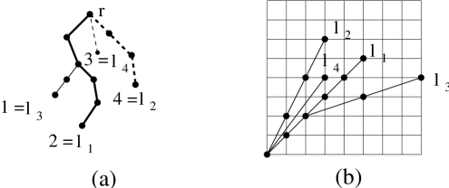
Figure 3: (a) The path decomposition of a tree $T$ with respect to the leaf-permutation $(2,4,1,3)$; (b) the drawing of $T$ produced by Algorithm 2 by using the vector set ${\cal V}=\{1/3,1/1,4/3,2/1\}$.

Fig 3 (a) shows a path decomposition of a tree with 4 leaves. The thick solid, thick dotted, thin solid and thin dotted lines correspond to $b_{1},b_{2},b_{3}$ and $b_{4}$, respectively. By a slight abuse of notation, we also use $b_{k}$ to denote the set of the vertices in path $b_{k}$ except the last vertex (the attachment vertex of $b_{k}$ in $T_{k}$). With this understanding, $\{b_{k}~{}|~{}1\leq k\leq t\}$ is also a partition of the vertex set of $T$.

Our Path Draw Algorithm is described in Algorithm 2.

Algorithm 2 Path Draw Algorithm

Input:

A tree $T=(V,E)$ and a set of paths $B_{\sigma}=\{b_{1},\ldots,b_{t}\}$ of $T$ with respect to a permutation $L_{\sigma}$ of the leaves in $T$.

1.

Take any set ${\cal V}=\{(x_{1},y_{1}),\ldots,(x_{t},y_{t})\}$ of $t$ distinct primitive vectors, sorted by increasing $y_{i}/x_{i}$ value.

2.

Assign the vectors in ${\cal V}$ to the leaves of $T$ in ccw order. (For example, in Fig 3 (a), the leaves $l_{3},l_{1},l_{4},l_{2}$ are assigned the 1st, 2nd, 3rd and the 4th vector in ${\cal V}$.)

2.1.

Let $(x,y)$ be the vector assigned to $l_{j}$ in step 2. Assign the vector $(x,y)$ to all edges in $b_{j}$. (We say the vector $(x,y)$ is assigned to the path $b_{j}$). Do the same for every path $b_{j}$ in $B$. Every edge in $T$ is assigned a vector in ${\cal V}$ by now.

3.

Draw the vertices of $T$ as in step 3 of Algorithm 1.

Fig 2 (d) shows the drawing of the tree in Fig 2 (a) produced by Algorithm 2 (by using the vectors in $\overline{P_{3}}$, and the permutation that lists the leaves in ccw order). Fig 3 (b) shows the drawing of the tree in Fig 3 (a) by Algorithm 2 by using the vector set ${\cal V}=\{1/3,1/1,4/3,2/1\}$.

Theorem 2

Algorithm 2 produces a monotone drawing of a tree $T$ for any permutation $L_{\sigma}$ of the leaves of $T$.

Proof: Consider two vertices $i,j$ in $T$. Let $P_{ij}$ be the (unique) path in the drawing of $T$ from $i$ to $j$. We need to show $P_{ij}$ is a monotone path. If either $i$ is an ancestor of $j$, or $j$ is an ancestor of $i$, this is trivially true (because every edge in $P_{ij}$ has angle between $0^{\circ}$ and $90^{\circ}$). So we assume this is not the case.

Let $u$ be the lowest common ancestor of $i$ and $j$ in $T$. Since any subpath of a monotone path is monotone [1], without loss of generality, we assume both $i$ and $j$ are leaves of $T$, and $i$ is located to the left of $j$ ($i$ appears before $j$ in ccw order) in the drawing. See Fig 4 (a).

Let $P_{iu}$ ($P_{uj}$, respectively) be the subpath of $P_{ij}$ from $i$ to $u$ (from $u$ to $j$, respectively). Consider any edge $e_{a}\in P_{iu}$ and any edge $e_{b}\in P_{uj}$. Let $\overline{e_{a}}$ be the edge $e_{a}$ but in opposite direction (i.e., directed away from the root). Then, $\overline{e_{a}}$ belongs to a path $b_{i^{\prime}}$ and $e_{b}$ belongs to a path $b_{j^{\prime}}$ in the path decomposition. It is easy to see that $b_{i^{\prime}}$ must appear to the left of $b_{j^{\prime}}$. Thus: $\operatorname{angle}(\overline{e_{a}})<\operatorname{angle}(e_{b})\mbox{ and }\operatorname{angle}(e_{a})=\operatorname{angle}(\overline{e_{a}})+180^{\circ}$.

Let $e_{\min}$ and $e_{\max}$ be the two extremal edges in $P_{ij}$ with $\operatorname{angle}(e_{\min})<\operatorname{angle}(e_{\max})$. Then, $e_{\max}$ must be an edge $e_{a}$ in $P_{iu}$ and $e_{\min}$ must be an edge $e_{b}$ in $P_{uj}$. By the above equation and inequality, we have: $\operatorname{angle}(e_{\max})-\operatorname{angle}(e_{\min})=\operatorname{angle}(\overline{e_{a}})+180^{\circ}-\operatorname{angle}(e_{b})<180^{\circ}$. By Property 2, $P_{ij}$ is a monotone path as to be shown. $\Box$

Figure 4: (a) The proof of Theorem 2; (b) the proof of Lemma 1.

3.2 Length Decreasing Path Decomposition of $T$

In this subsection, we define a special path decomposition of $T$, called the length decreasing path decomposition and denoted by LDPD. Later, we will apply Algorithm 2 with respect to this decomposition. Note that LDPD is a special case of the well-known heavy path decomposition [17]. However, our algorithm does not need any operation provided by heavy path decomposition, only the definition.

Definition 3

A length decreasing path decomposition $B=\{b_{1},b_{2},...,b_{t}\}$ of a tree $T$ is defined as follows:

1. Let $l_{1}$ be the vertex that is the farthest from the root $r$ of $T$ (break ties arbitrarily). Define $b_{1}$ as the path from $l_{1}$ to $r$.

2. Suppose that the leaves $l_{1},\ldots,l_{k}$ and the corresponding paths $b_{1},\ldots,b_{k}$ have been defined. Let $T_{k}=\cup_{i=1}^{k}b_{i}$. Let $l_{k+1}$ be the leaf in $L-\{l_{1},\ldots,l_{k}\}$ such that the path from $l_{k+1}$ to its attachment $u$ in $T_{k}$ is the longest among all leaves in $L-\{l_{1},\ldots,l_{k}\}$ (break ties arbitrarily). Define $b_{k+1}$ as the path from $l_{k+1}$ to $u$.

Fig 3 (a) shows a LDPD of a tree. Let $|b_{i}|$ denote the number of edges in $b_{i}$. By definition, we have $|b_{i}|\geq|b_{i+1}|$ for $1\leq i<t$. We further partition the paths in $B$ as follows.

Definition 4

Let $T$ be a $n$-vertex tree and $B=\{b_{1},b_{2},...,b_{t}\}$ be a LDPD of $T$. Let $c>1$ be an integer and $K=\lceil\log_{c}n\rceil$. The $c$-partition of $B$ is a partition of $B$ defined as:

$$D_{1} = \{b_{i}\in B~{}|~{}|b_{i}|\in[\frac{n-1}{c},(n-1)]\}$$

$$D_{j} = \{b_{i}\in B~{}|~{}|b_{i}|\in[\frac{n-1}{c^{j}},\frac{n-1}{c^{j-1}})\},\mbox{ for }1<j\leq K$$

Note that $D_{j}$’s are disjoint and $\cup_{j=1}^{K}D_{j}=B$. Let $m_{j}=|D_{j}|$ ($1\leq j\leq K$) be the number of paths in $D_{j}$. We have the following:

Property 3

$c^{K-1}\leq\sum_{j=1}^{K}m_{j}c^{K-j}\leq c^{K}$.

Proof: For each $j$ ($1\leq j\leq K$), there are $m_{j}$ paths in $D_{j}$. Each path $b_{l}\in D_{j}$ contains $|b_{l}|\in[\frac{n-1}{c^{j}},\frac{n-1}{c^{j-1}})$ edges. Thus we have:

$$\sum_{j=1}^{K}m_{j}\frac{n-1}{c^{j}}\leq n-1=\sum_{j=1}^{K}\sum_{{b_{l}}\in D_{j}}|b_{l}|\leq\sum_{j=1}^{K}m_{j}\frac{n-1}{c^{j-1}}$$

Hence $\sum_{j=1}^{K}\frac{m_{j}}{c^{j}}\leq 1\leq\sum_{j=1}^{K}\frac{m_{j}}{c^{j-1}}$. This implies the property. $\Box$

For each $j$, let $T[D_{j}]$ denote the subgraph of $T$ induced by the edge set $\cup_{b_{l}\in D_{j}}b_{l}$. $T[D_{j}]$ may consist of several subtrees in $T$. We call the subtrees in $T[D_{j}]$ the $j$-level subtrees of $T$. We have:

Lemma 1

For any $j$ ($1\leq j\leq K$), let $t_{j}$ be the subtree among all $j$-level subtrees with the largest height $h_{j}$. Then, $h_{j}<\frac{n-1}{c^{j-1}}$.

Proof: For a contradiction, suppose $h_{j}\geq\frac{n-1}{c^{j-1}}$. Let $l_{p}$ be the leaf in $t_{j}$ with the largest distance to the attachment $u$ of $t_{j}$. So the length of the path from $l_{p}$ to $u$ is $h_{j}\geq\frac{n-1}{c^{j-1}}$. See Fig 4 (b). By the definition of the LDPD, $l_{p}$ should have been chosen as $l_{q}$ for some index $q<p$ such that $|b_{q}|\geq\frac{n-1}{c^{j-1}}$. This contradiction shows the assumption $h_{j}\geq\frac{n-1}{c^{j-1}}$ is false. $\Box$

3.3 Vector Assignment

We will use Algorithm 2 with respect to a LDPD $B=\{b_{1},\ldots,b_{t}\}$ of $T$. First, we need the following definition:

Definition 5

Two positive integers $(f,d)$ are called a valid-pair if the following hold:

1. $f\geq d$;

2. For any positive integer $\Delta$ and any two consecutive vectors $(x_{1},y_{1})$ and $(x_{2},y_{2})$ in $\overline{P_{\Delta}}$ with $y_{1}/x_{1}<y_{2}/x_{2}$ (either one can be the boundary vector (0,1) or (1,0)), there exist at least $f$ vectors $(x,y)$ in $\overline{P_{d\Delta}}-\overline{P_{\Delta}}$ such that $y_{1}/x_{1}<y/x<y_{2}/x_{2}$.

Our algorithm works for any valid-pair $(f,d)$. Later we will show $(f,d)=(3,3)$ is a valid-pair. The main ideas of our algorithm are as follows. Take a valid-pair $(f,d)$. Set $c=f+1$ and let $K=\lceil\log_{c}n\rceil$. Let $T$ be a tree and $B=\{b_{1},\ldots,b_{t}\}$ be a LDPD of $T$. Let $D=\{D_{1},D_{2},...,D_{K}\}$ be the $c$-partition of $B$. The vectors in $\overline{P_{d^{j}}}-\overline{P_{d^{j-1}}}$ are called level-$j$ vectors (for $1\leq j\leq K$). In other words, the level-$j$ vectors are the vectors with size in the range $(d^{j-1},d^{j}]$. We assign the level-1 vectors to the paths in $D_{1}$. (Because the paths in $D_{1}$ are very long, we assign very short level-1 vectors to them). As the index $j$ becomes larger, the paths in $D_{j}$ are shorter. We can afford to assign longer level-$j$ vectors to the paths in $D_{j}$ without increasing the size of the drawing too much.

Next, we describe our algorithm in details. It first constructs a set ${\cal V}$ of primitive vectors as follows.

• There is only one primitive vector $(1,1)$ in $\overline{P_{1}}$. By the definition of the valid-pair, there exist at least $f$ vectors in $\overline{P_{d}}-\overline{P_{1}}$ between $(1,0)$ and $(1,1)$. Let $S_{1}$ be a set of $f$ vectors among them. Similarly, there exist at least $f$ vectors in $\overline{P_{d}}-\overline{P_{1}}$ between $(1,1)$ and $(0,1)$. Let $S_{2}$ be a set of $f$ vectors among them. Define $R_{1}=S_{1}\cup S_{2}\cup\{(1,1)\}$. Thus $|R_{1}|=2f+1$.

• Between any two consecutive vectors in $R_{1}\cup\{(0,1),(1,0)\}$, there are at least $f$ vectors in $\overline{P_{{d}^{2}}}-\overline{P_{{d}^{1}}}$. Pick exactly $f$ vectors among them. Let $R_{2}$ be the union of all vectors picked for all consecutive pairs. Thus $|R_{2}|=(2f+2)f$.

• Suppose we have defined $R_{1},\ldots,R_{j}$. Between any two consecutive vectors in $[\cup_{i=1}^{j}R_{i}]\cup\{(0,1),(1,0)\}$, there are at lease $f$ vectors in $\overline{P_{{d}^{j+1}}}-\overline{P_{{d}^{j}}}$. Pick exactly $f$ vectors among them. Let $R_{j+1}$ be the union of all vectors picked for all consecutive pairs. Thus $|R_{j+1}|=(1+\sum_{i=1}^{j}|R_{i}|)f$.

• Define ${\cal V}=\cup_{j=1}^{K}R_{j}$ (in increasing order of slopes).

Lemma 2

1. For any $p$ ($1\leq p\leq K$), $\sum_{j=1}^{p}|R_{j}|=2(f+1)^{p}-1$. (This implies $|{\cal V}|=2(f+1)^{K}-1$).

2. Let $j$ ($1\leq j\leq K$) be an integer. Consider any vector $V_{\alpha}$ in ${\cal V}$. Let $V_{\beta}$ be the first vector in ${\cal V}$ after $V_{\alpha}$ that is in $R_{i}$ with $i\leq j$. Then there are at most $(f+1)^{K-j}-1$ vectors in ${\cal V}$ between $V_{\alpha}$ and $V_{\beta}$.

Proof: Statement 1: We prove the equality by induction on $p$.

When $p=1$, $|R_{1}|=2f+1=2(f+1)-1$ is trivially true.

Assume $\sum_{j=1}^{p}|R_{j}|=2(f+1)^{p}-1$.

Then: $\sum_{j=1}^{p+1}|R_{j}|=(\sum_{j=1}^{p}|R_{j}|)+|R_{p+1}|=(2(f+1)^{p}-1)+(2(f+1)^{p}-1+1)f=2(f+1)^{p+1}-1$ as to be shown.

Statement 2: Let $S$ be the set of the vectors in ${\cal V}$ that are between $V_{\alpha}$ and $V_{\beta}$. The worst case (that $S$ has the largest size) is when $V_{\alpha}$ itself is a level-$j$ vector. In this case, $S$ contains $f$ level-$(j+1)$ vectors, $(f+1)f$ level-$(j+2)$ vectors, $\ldots$ and so on. By using induction similar to the proof of Statement 1, we can show $|S|=(f+1)^{K-j}-1$. $\Box$

Let $b_{1},\ldots,b_{t}$ be the paths in a LDPD of $T$ ordered from left to right. We call $b_{l}$ a level-$j$ path if $b_{l}\in D_{j}$. We will assign the vectors in ${\cal V}$ to the paths $b_{l}$ ($1\leq l\leq t$) such that the following properties hold:

• The vectors in ${\cal V}$ (in the order of increasing slopes) are assigned to $b_{l}$’s in ccw order.

• For each level-$j$ path $b_{l}$, $b_{l}$ is assigned a vector in $R_{i}$ with $i\leq j$.

3.4 Algorithm

Now we present our optimal monotone drawing Algorithm for trees.

Algorithm 3 Optimal Draw

Input:

A tree $T=(V,E)$, and a valid-pair ($f,d$).

1.

Find a LDPD $B=\{b_{1},\ldots b_{t}\}$ of $T$ (ordered from left to right).

2.

Set $c=f+1$ and let $K=\lceil\log_{c}n\rceil$. Construct the $c$-partition $D=\{D_{1},\ldots,D_{K}\}$ of $B$.

3.

Let ${\cal V}$ be the set of primary vectors (in increasing order of slops) defined in subsection 3.3.

4.

For $l=1$ to $t$ do:

If $b_{l}$ is a level-$j$ path, assign the next available (skip some vectors in ${\cal V}$ if necessary) vector in ${\cal V}$ that is in $R_{i}$ with $i\leq j$.

5.

Draw the vertices of $T$ as in step 3 of Algorithm 1.

It is not clear whether there are enough vectors in ${\cal V}$ such that the vector assignment procedure described in Algorithm 3 can succeed. The following lemma shows this is indeed the case.

Lemma 3

There are enough vectors in ${\cal V}$ such that the vector assignment procedure in Algorithm 3 can be done.

Proof: Consider a level-$j$ path $b_{l}$. In order to assign a vector $V_{\beta}\in{\cal V}$ to $b_{l}$, we may have to skip at most $(f+1)^{K-j}-1$ vectors in ${\cal V}$ by Lemma 2. Also counting the vector $V_{\beta}$ assigned to $b_{l}$, we consume at most $(f+1)^{K-j}$ vectors in ${\cal V}$. Thus the total number of vectors needed by the vector assignment procedure is bounded by:

$$\sum_{j=1}^{K}m_{j}\cdot(f+1)^{K-j}=\sum_{j=1}^{K}m_{j}\cdot c^{K-j}\leq c^{K}\mbox{ (by Property \ref{prop:partition})}\leq 2c^{K}-1=|{\cal V}|\mbox{ (by Lemma \ref{lemma:size}.)}$$

Thus, there are enough vectors in ${\cal V}$ for the vector assignment procedure in Algorithm 3. $\Box$

Now we can prove our main theorem:

Theorem 3

For any valid-pair $(f,d)$, Algorithm 3 constructs a monotone drawing of $T$ with size $I\times I$, where $I\leq\frac{(f+1)\cdot d}{(f+1)-d}n$, in $O(n)$ time.

Proof: Because the vector assignments in Algorithm 3 satisfy the condition required by Algorithm 2, it indeed produces a monotone drawing of $T$ by Theorem 2. It’s straightforward to show that the algorithm takes $O(n)$ time by using basic algorithmic techniques as in [1, 9]. Next, we analyze the size of the drawing.

The subgraph $T[D_{1}]$ is a subtree of $T$ with height at most $n-1<n$. The paths in $D_{1}$ are assigned the vectors of length at most $d$. So, Algorithm 3 draws the level-1 subtree $T[D_{1}]$ on a grid of size at most $d\cdot n\times d\cdot n$.

In general, the height of any subtree in the subgraph $T[D_{j}]$ is at most $(n-1)/c^{j-1}<n/c^{j-1}$ (where $c=f+1)$ by Lemma 1. The paths in $D_{j}$ are assigned the vectors of length at most $d^{j}$. So Algorithm 3 can draw the level-$j$ subtrees in $T[D_{j}]$, increasing the size of the drawing by at most $d\cdot(d/c)^{j-1}\cdot n$ in both $x$- and $y$-direction.

So, Algorithm 3 draws $T$ on an $I\times I$ grid, where $I\leq n\cdot d\cdot\sum_{j=1}^{K}(d/c)^{j-1}<\frac{c\cdot d}{c-d}n=\frac{(f+1)\cdot d}{(f+1)-d}n$. $\Box$

3.5 The Existence of Valid-pairs

Let $F_{0}=1,F_{1}=1,F_{2}=F_{0}+F_{1}=2,\ldots,F_{i+2}=F_{i+1}+F_{i}\ldots$ be the Fibonacci numbers. In this subsection, we show:

Lemma 4

For any integer $q\geq 2$, $(2^{q}-1,F_{q+1})$ is a valid-pair.

Proof: Fix a positive integer $\Delta$. Let $y_{1}/x_{1}$ and $y_{2}/x_{2}$ be any two consecutive vectors in $\overline{P_{\Delta}}$. We have $y_{2}x_{1}-y_{1}x_{2}=1$ ([8], Theorem 28) and $x_{1}+x_{2}>\Delta$ ([8], Theorem 30).

Define an operator $\odot$ of two fractions as follows:

$$\frac{y_{1}}{x_{1}}\odot\frac{y_{2}}{x_{2}}=\frac{y_{1}+y_{2}}{x_{1}+x_{2}}$$

Let $y_{3}/x_{3}=\frac{y_{1}}{x_{1}}\odot\frac{y_{2}}{x_{2}}$. It is easy to show that $y_{3}/x_{3}$ is a fraction strictly between $y_{1}/x_{1}$ and $y_{2}/x_{2}$. Similarly, let $y_{4}/x_{4}=y_{1}/x_{1}\odot y_{3}/x_{3}$ and $y_{5}/x_{5}=y_{3}/x_{3}\odot y_{2}/x_{2}$, we have three fractions $y_{4}/x_{4}<y_{3}/x_{3}<y_{5}/x_{5}$ strictly between $y_{1}/x_{1}$ and $y_{2}/x_{2}$.

Repeating this process, we can generate all fractions between $y_{1}/x_{1}$ and $y_{2}/x_{2}$ in the form of a binary tree, called the Stern-Brocot tree for $y_{1}/x_{1}$ and $y_{2}/x_{2}$, denoted by ${\cal T}(y_{1}/x_{1},y_{2}/x_{2})$, as follows. (The original Stern-Brocot tree defined in [5, 18] is for the fractions $y_{1}/x_{1}=0/1$ and $y_{2}/x_{2}=1/0$).

${\cal T}(y_{1}/x_{1},y_{2}/x_{2})$ has two nodes $y_{1}/x_{1}$ and $y_{2}/x_{2}$ in level 0. Level 1 contains a single node $r$ labeled by the fraction $y_{3}/x_{3}=y_{1}/x_{1}\odot y_{2}/x_{2}$, which is the right child of $y_{1}/x_{1}$, and is the left child of $y_{2}/x_{2}$. An infinite ordered binary tree rooted at $y_{3}/x_{3}$ is constructed as follows. Consider a node $y/x$ of the tree. The left child of $y/x$ is $y/x\odot y^{\prime}/x^{\prime}$ where $y^{\prime}/x^{\prime}$ is the ancestor of $y/x$ that is closest to $y/x$ (in terms of graph-theoretical distance in ${\cal T}(y_{1}/x_{1},y_{2}/x_{2})$) and that has $y/x$ in its right subtree. The right child of $y/x$ is $y/x\odot y^{\prime\prime}/x^{\prime\prime}$ where $y^{\prime\prime}/x^{\prime\prime}$ is the ancestor of $y/x$ that is closest to $y/x$ and that has $y/x$ in its left subtree. (Fig 5 shows a portion of the Stern-Brocot tree ${\cal T}(4/5,5/6)$. The leftmost column indicates the level numbers).

Figure 5: The first 5 levels of the Stern-Brocot tree ${\cal T}(4/5,5/6)$.

The following facts are either from [5, 18]; or directly from the definition of ${\cal T}(y_{1}/x_{1},y_{2}/x_{2})$; or can be shown by easy induction:

1. All fractions in ${\cal T}(y_{1}/x_{1},y_{2}/x_{2})$ are distinct primitive vectors and are strictly between $y_{1}/x_{1}$ and $y_{2}/x_{2}$.

2. Each node in level $k$ is the result of the operator $\odot$ applied to a node in level $k-1$ and a node in level $\leq k-2$.

3. In each level $k$, there exists a node that is the result of the operator $\odot$ applied to a node in level $k-1$ and a node in level $k-2$.

4. Let ${\cal T}_{q}$ be the subtree of ${\cal T}(y_{1}/x_{1},y_{2}/x_{2})$ from level 1 through level $q$. Let ${\cal V}_{q}$ be the set of the fractions contained in ${\cal T}_{q}$. Then $|{\cal V}_{q}|=2^{q}-1$.

5. For each node $y/x$ with the left child $y^{\prime}/x^{\prime}$ and the right child $y^{\prime\prime}/x^{\prime\prime}$, we have $y^{\prime}/x^{\prime}<y/x<y^{\prime\prime}/x^{\prime\prime}$. So the in-order traversal of ${\cal T}_{q}$ lists the fractions in ${\cal V}_{q}$ in increasing order.

6. Define the size of a node $y/x$ to be $\max\{x,y\}$. The size of the nodes in level 0 (i.e., the two nodes $y_{1}/x_{1}$ and $y_{2}/x_{2}$) is bounded by $1\cdot\Delta=F_{1}\cdot{\Delta}$ (because both $y_{1}/x_{1}$ and $y_{2}/x_{2}$ are fractions in $\overline{P_{\Delta}}$).

7. The size of the node in level 1 (i.e., the node $y_{3}/x_{3}$) is bounded by $2\cdot\Delta=F_{2}\cdot\Delta$ (because $x_{3}=x_{1}+x_{2}\leq 2\Delta$ and $y_{3}=y_{1}+y_{2}\leq 2\Delta$).

8. For each $q\geq 2$, the size of level $q$ nodes is bounded by $F_{q+1}\cdot\Delta$. (The last column in Fig 5 shows the upper bounds of the size of the level $q$ fractions.)

The lemma immediately follows from the above facts 1, 4 and 8. $\Box$

Corollary 1

Every $n$-vertex tree $T$ has a monotone drawing on a grid of size at most $12n\times 12n$.

Proof: By Lemma 4, $(3,3)$ is a valid-pair. Take this valid-pair, the corollary follows from Theorem 3. $\Box$

4 Lower Bound

Let $T_{0}$ be a tree with root $r$ and 12 edge-disjoint paths $P_{1},P_{2},...,P_{12}$, and each $P_{i}$ has $\frac{n}{12}$ vertices. In this section, we show that any monotone drawings of $T_{0}$ must use a grid of size $\Omega(n)\times\Omega(n)$. Hence, our result in Section 3 is asymptotically optimal.

Lemma 5

There exists a tree $T_{0}$ with $n$ vertices such that every monotone drawing of $T_{0}$ must use an $\Omega(n)\times\Omega(n)$ grid.

Proof: Let $e_{i}$ ($1\leq i\leq 12$) be the first edge in $P_{i}$ (see Fig 6 (a)). Let $\Gamma$ be any monotone drawing of $T_{0}$. Without loss of generality, we assume the root $r$ is drawn at the origin $(0,0)$.

Figure 6: (a) A tree $T_{0}$ with 12 edge-disjoint paths; (b) the proof of Lemma 5.

By pigeonhole principle, at least three edges $e_{i}$ must be drawn in the same quadrant. Without loss of generality, we assume the edges $e_{1},e_{2}$ and $e_{3}$ are drawn in the first quadrant in ccw order. Let $e_{1}=(r,v)$, $e_{3}=(r,w)$, and $r=u_{0},u_{1},\ldots,u_{k}$ ($k=n/12$) be the vertices of $P_{2}$. Thus $e_{2}=(r,u_{1})$, and $0^{\circ}\leq\operatorname{angle}(r,v)<\operatorname{angle}(r,u_{1})<\operatorname{angle}(r,w)\leq 90^{\circ}$ (see Fig 6 (b)).

Consider the tree path $Q_{1}$ from $v$ to $u_{i}$ (for any index $1\leq i\leq k$). Let $e^{1}_{\min}$ and $e^{1}_{\max}$ be the two extremal edges of $Q_{1}$ with $\operatorname{angle}(e^{1}_{\min})<\operatorname{angle}(e^{1}_{\max})$. Since $Q_{1}$ is monotone, we must have $\operatorname{angle}(e^{1}_{\max})-\operatorname{angle}(e^{1}_{\min})<180^{\circ}$ by Property 2. Note that $\operatorname{angle}(e^{1}_{\max})\geq\operatorname{angle}(v,r)\geq 180^{\circ}$. This implies $\operatorname{angle}(u_{i-1},u_{i})\geq\operatorname{angle}(e^{1}_{\min})>\operatorname{angle}(e^{1}_{\max})-180^{\circ}\geq 0^{\circ}$.

Now consider the tree path $Q_{2}$ from $u_{i}$ to $w$. Let $e^{2}_{\min}$ and $e^{2}_{\max}$ be the two extremal edges of $Q_{2}$ with $\operatorname{angle}(e^{2}_{\min})<\operatorname{angle}(e^{2}_{\max})$. Since $Q_{2}$ is monotone, we must have $\operatorname{angle}(e^{2}_{\max})-\operatorname{angle}(e^{2}_{\min})<180^{\circ}$ by Property 2. Note that $\operatorname{angle}(e^{2}_{\min})\leq\operatorname{angle}(r,w)\leq 90^{\circ}$. This implies $\operatorname{angle}(u_{i},u_{i-1})\leq\operatorname{angle}(e^{2}_{\max})<\operatorname{angle}(e^{2}_{\min})+180^{\circ}\leq 270^{\circ}$. Hence, $\operatorname{angle}(u_{i-1},u_{i})<90^{\circ}$.

Thus, for every edge $(u_{i-1},u_{i})\in P_{2}$, $0^{\circ}<\operatorname{angle}(u_{i-1},u_{i})<90^{\circ}$. Let $(x(u_{i-1}),y(u_{i-1}))$ and $(x(u_{i}),y(u_{i}))$ be the two points in the drawing $\Gamma$ corresponding to $u_{i-1}$ and $u_{i}$, respectively. Because $0^{\circ}<\operatorname{angle}(u_{i-1},u_{i})<90^{\circ}$, we have $x(u_{i})-x(u_{i-1})\geq 1$ and $y(u_{i})-y(u_{i-1})\geq 1$. So, in order to draw $P_{2}$, we need a grid of size at least $\frac{n}{12}\times\frac{n}{12}$ in the first quadrant. $\Box$

5 Conclusion

In this paper, we showed that any $n$-vertex tree has a monotone drawing on a $12n\times 12n$ grid. The drawing can be constructed in $O(n)$ time. We also described a tree $T_{0}$ and showed that any monotone drawing of $T_{0}$ must use a grid of size at least $\frac{n}{12}\times\frac{n}{12}$. So the size of our monotone drawing of trees is asymptotically optimal.

It is moderately interesting to close the gap between the lower and the upper bounds on the size of monotone drawing for trees. To reduce the constant in the drawing size, one possible approach is to improve Lemma 4, whose proof is not tight. In the Stern-Brocot tree ${\cal T}$, the sizes of the nodes near the leftmost and the rightmost path of ${\cal T}$ are (much) smaller than the bound stated in the proof of Lemma 4. So it is possible to prove that $(2^{q}-1+t,F_{q+1})$ is a valid-pair for some integer $t$ ($t$ depends on $q$). By using these better valid-pairs in Theorem 3, it is possible to reduce the constant in the size of the drawing.

References

- [1] P. Angelini, E. Colasante, G. Di Battista, F. Frati and M. Patrignani, Monotone Drawings of Graphs, J. of Graph Algorithms and Appl. vol. 16, no. 1, pp. 5–35, 2012.
- [2] P. Angelini, F. Frati and L. Grilli, An Algorithm to Construct Greedy Drawings of Triangulations, J. of Graph Algorithms and Appl. vol. 14, no. 1, pp. 19–51, 2010.
- [3] P. Angelini, W. Didimo, S. Kobourov, T. Mchedlidze, V. Roselli, A. Symvonis, and S. Wismath, Monotone Drawings of Graphs with Fixed Embedding, Algorithmica, DOI 10.1007/s00453-013-9790-3, 2013.
- [4] E. M. Arkin, R. Connelly and J.S. Mitchell, On Monotone Paths among Obstacles with Applications to Planning Assemblies, SoCG ’89, pp. 334–343, 1989.
- [5] A. Brocot, Calcul des Rouages par Approximation, Nouvelle Methode, Revue Chronometrique, vol 6. pp. 186–194, 1860.
- [6] G. Di Battista and R. Tamassia, Algorithms for Plane Representations of Acyclic Digraphs, Theor. Comput. Sci. vol. 61, pp. 175–198, 1988.
- [7] A. Garg and R. Tammassia, On the Computational Complexity of Upward and Rectilinear Planarity Testing, SIAM J. Comp. vol. 31 (2), pp. 601–625, 2001
- [8] G. Hardy and E. M. Wright, An Introduction to the Theory of Numbers, 5th Edition, Oxford University Press, 1989.
- [9] X. He and D. He, Compact Monotone Drawing of Trees, in Proceedings of COCOON 2015, LNCS 9198, pp. 457–468, 2015.
- [10] X. He and D. He, Monotone Drawing of 3-Connected Plane Graphs, in Proceedings of ESA 2015, LNCS 9294, pp. 729–741, 2015.
- [11] Md. Iqbal Hossain and Md. Saidur Rahman, Monotone Grid Drawings of Planar Graphs, in Proceedings of FAW 2014, LNCS 8497, pp. 105–116, 2014.
- [12] W. Huang, P. Eades and S.H. Hong, A Graph Reading Behavior: Geodesic-Path Tendency, in Proceedings of IEEE Pacific Visualization Symposium, pp. 137–144, 2009.
- [13] P. Kindermann, A. Schulz, J. Spoerhase and A. Wolff, On Monotone Drawings of Trees, in Proceedings of GD 2014, LNCS 8871, pp. 488–500, 2014.
- [14] A. Moitra and T. Leighton, Some Results on Greedy Embeddings in Metric Spaces, in Proceedings FOCS 2008, pp. 337–346, 2008.
- [15] M. Nöllenburg, R. Prutkin, and I. Rutter, On Self-Approaching and Increasing-Chord Drawings of 3-Connected Planar Graphs, in Proceedings GD 2014, LNCS 8871, pp. 476–487.
- [16] C. H. Papadimitriou and D. Ratajczak, On a Conjecture Related to Geometric Routing, Theor. Comput. Sci., vol. 344 (1), pp. 3–14, 2005.
- [17] D.D. Sleator and R.E. Tarjan, A data structure for dynamic trees, J. of Computer and System Sciences, vol. 24, pp. 362–391, 1983.
- [18] M. A. Stern, Über eine Zahlentheoretische Funktion, Journal für die reine und angewandte Mathematik vol. 55, pp. 193–220, 1958.