Breaking the color-reddening degeneracy in type Ia supernovae

Abstract

A new method to study the intrinsic color and luminosity of type Ia supernovae (SNe Ia) is presented. A metric space built using principal component analysis (PCA) on spectral series SNe Ia between $-12.5$ and $+17.5$ days from $B$ maximum is used as a set of predictors. This metric space is built to be insensitive to reddening. Hence, it does not predict the part of color excess due to dust-extinction. At the same time, the rich variability of SN Ia spectra is a good predictor of a large fraction of the intrinsic color variability. Such metric space is a good predictor of the epoch when the maximum in the $B-V$ color curve is reached. Multivariate Partial Least Square (PLS) regression predicts the intrinsic $B$ band light-curve and the intrinsic $B-V$ color curve up to a month after maximum. This allows to study the relation between the light curves of SNe Ia and their spectra. The total-to-selective extinction ratio R_V in the host-galaxy of SNe Ia is found, on average, to be consistent with typical Milky-Way values. This analysis shows the importance of collecting spectra to study SNe Ia, even with large sample publicly available. Future automated surveys as LSST will provide a large number of light curves. The analysis shows that observing accompaning spectra for a significative number of SNe will be important even in the case of “normal” SNe Ia.

1 Introduction

The use of type Ia supernovae (SNIa) as standardizable candles provided the first evidence of an accelerated expansion of the Universe in late 20^th century (Riess et al., 1998; Perlmutter et al., 1999). Since these first results were presented the standardization procedure improved considerably, allowing for tighter constraints over cosmological parameters. Consequently, we have reached a point where the intrinsic characteristics of the SNe can not be neglected if we wish to improve the calibration and take into account systematic effects. The colour-dust connection is one such bottleneck.

The typical total to selective extinction estimate from Milky-Way measurements, $R_{V}=3.1$, is significantly different from the one obtained from SNIa Hubble residuals, $1.7<R_{V}<2.5$. This discrepancy has been attributed to a poor understanding of the intrinsic color variability or to unusual extragalactic or interstellar dust. Disentangling extrinsic and intrinsic variations in SNIa samples is a difficult and essential problem, which might impact calibration for all subsequent cosmological parameters estimations.

Chotard et al., 2011 showed that corrections of the intrinsic color derived for individual analysis of equivalent widths may lead to an $R_{V}$ estimated from SNIa which agrees with standard Milky-Way values. In this paper, we improved upon the techniques presented in Sasdelli et al. (2015) and use the correlations between spectral series and light curves to study the behaviour of the $B-V$ color curve and the host-galaxy total-to-selective extinction ratio $R_{V}$ of SNe Ia. Our method uses a data set of spectra series and light curves in order to estimate a color law for SNe Ia. Once this is determined, the identification of how much of the color is due to dust and how much of it is due to intrinsic properties is straightforward for an object with spectroscopic observations.

The core argument presented in Sasdelli et al. (2015) relies on finding correlations between spectral series and light curve measurements on the same set of SNe Ia. The radiation transport physics that forms the spectra is a complex phenomenon. A lot of information on the physical structure of the ejecta is encoded in its spectral features and their time evolution. However, using this information in the spectra to measure the amount of extinction and the type of dust along the line of sight is not an easy task. The differences in the shape of the spectral features are hard to quantify systematically. It is clear that this spectral variability correlates with the intrinsic color. In the literature a number of predictors have been suggested and studied with the aim of predicting the intrinsic color. A simple method to study the color is to select a subsample of objects believed to have little or no reddening, and use them as a template (e.g: Reindl et al., 2005; Folatelli et al., 2010). More advanced methods involve the use of one or more spectral features as predictors of the intrinsic color (e.g. Nordin et al., 2011; Foley et al., 2011; Chotard et al., 2011). For example, the velocity of the Si ii 6355 Å (Foley & Kasen, 2011; Mandel et al., 2014). Finally, other methods are based on multi color light-curves (e.g Riess et al., 1996a, b; Ganeshalingam et al., 2010). The Lira-relationship is an example of such an approach (Phillips et al., 1999) The properties of the extinction have also been studied with a statistical approach based on light curves (Scolnic et al., 2014).

To extract the intrinsic color from the spectra is not a simple task. Partially, this is due to the difficulty in calibrating data obtained by slit spectroscopy. Even when flux calibrated spectra are available, it is difficult to separate the variability of intrinsic color and luminosity from dust-extinction. For a given spectral type, the intrinsic spectrum is the “bluest” in the data. Extinction makes the spectra redder and fainter. However, when two spectra are “different”, the intrinsic color may be different. The difficult part is quantify what “different” and “similar” mean when the spectra show a continuum distribution of properties.

Photometry can be used to construct light curves of SNe in different bands, providing an indirect proxy of its spectral energy distribution. A fraction of the spectrum intrinsic variability is encoded in the photometry too. Most importantly, all the information about the extinction (type and amount of extinction) is encoded in the light curves. Also in this case it is difficult to disentangle the intrinsic variability, which has to correlate with spectral features, from the extrinsic variability due to dust extinction which affects the overall shape of the spectrum.

Our approach not only finds doubles of SNe with different extinction and similar spectal properties. We use the reasonable assumption that when you have a SN with spectral characteristics that are intermediate between other two SNe, the intrinsic color is also intermediate between the two. To find the function between the space of the spectra and the color curves we use a technique called Partial Least Square regression (PLS). We use PLS to find the latent structures connecting these two spaces and to predict the intrinsic component of the light curves from series of spectra. As shown by Sasdelli et al. (2015) the data compression of the spectral series is handled with the help of Expectation Maximization Principal Component Analysis (EMPCA) and derivative spectroscopy.

The paper is organized as follows. Section 2 illustrates the SN data used in our analysis. Section 3 explains the technique used. Section 4 shows the results on SN Ia data. Section 5 wraps up the conclusions and future applications.

2 The type Ia supernova data

For this work we collected most of the currently publicly available visible spectra and B and V band photometry of SNe Ia. Our sources of spectra are the CfA spectroscopic release (Blondin et al., 2012), the Berkleley Supernova Program (Silverman et al., 2012), the Carnegie Supernova Project (CSP, Folatelli et al., 2013). We make use of the SN repositories SUSPECT and WISEREP (Yaron & Gal-Yam, 2012). The spectra are deredshifted using the heliocentric redshifts published in Blondin et al. (2012). CSP spectra are published deredshifted.

We collect the $B$ and $V$ band photometry published in Hicken et al. (2009) and Stritzinger et al. (2011). The redshift of most of the sample is lower than $z=0.04$. The central wavelength of the filters in the observer frame is only marginally different from the corresponding wavelength in the rest frame. To check the importance of this effect, we performed the analysis with and without K-corrections on the photometry and in our sample the outcome is not significantly affected by this second order correction. Of course, to study samples at high redshift, a careful K-correction becomes a necessity. We check how important is to correct the photometry into rest frame before comparing our SNe Ia. We apply a K-correction that converts the magnitude to rest frame. As a first order approximation, we have chosen to use the spectra of SN 2011fe (Mazzali et al., 2014) as a template to calculate all of the K-corrections. We shift the flux calibrated spectra of SN 2011fe to the redshift of the SN that we want to correct. Then, we calculate the K-correction factor at each epoch using the method from Oke & Sandage (1968); Hogg et al. (2002), and apply the relative K-correction to the photometric data at the nearest epoch. Applying K-corrections to our sample does not affect significantly our results, as it affects the fluxes in the studied bands by less than 5% in most cases.

We deredden the photometry from the Milky Way extinction using (Schlegel et al., 1998; Schlafly & Finkbeiner, 2011). The host galaxy extinction, the subject of our study, is not estimated or removed from the photometry during this step.

To calculate the absolute magnitudes of the SNe we use CMB centered redshift measurements from Hicken et al. (2009) and assume a smooth Hubble flow. We are only interested in differences between absolute magnitudes. This makes it unnecessary to know the actual value of the Hubble constant. The error on the absolute magnitude due to the peculiar motion of each host galaxy is assumed to be 500 km s^-1 (Hawkins et al., 2003).

3 The method: predicting light curves with spectral series

This section summarizes the techniques used to construct a metric space for SN Ia spectral series (Sasdelli et al., 2015) and to predict the intrinsic part of their light and color curves.

3.1 Principal Component Analysis to construct a metric space for type Ia spectral series

We follow closely the techniques explained in details in Sasdelli et al. (2015). In this subsection we recap how to create a metric space for SN Ia spectral series.

In the literature a large number of visible spectra of SNe Ia taken few weeks around maximum brightness is available. Most of these spectra are obtained by means of slit spectroscopy and many are not flux calibrated (e.g. Blondin et al., 2012). The spectra have been obtained with a number of different instruments by many surveys over a time frame of decades. This means that the wavelength coverage is not constant, the signal-to-noise ratio is diverse, and the time sampling of the SNe is not uniform. The approach of Sasdelli et al. (2015) offers a solution for these problems and it creates a meaningful metric space for SN Ia spectral series.

We perform the following algorithms that lead to the creation of our metric space. First, we calculate the derivative over lambda of the spectra ($\frac{d\log_{10}F_{\lambda}}{d\lambda}$). The reason is to retain all the small scale information present in the spectra, without the problem of the uncertainty on the distance and of the absolute flux calibration of the spectra. Also, in the derivative space, the weight given to long scale variations in the flux is reduced. The knowledge of the amount of extinction and the type of dust becomes unnecessary. Most importantly, flux calibration of the spectra is also not necessary.

Figure 1: The figure shows the spectral evolution of the prototypical normal SN Ia, SN1994D. The evolution of the spectrum was followed from two weeks before maximum up to few hundred days after. The “square” delineated in red highlights the spectral variability that we include in our statistical analysis.

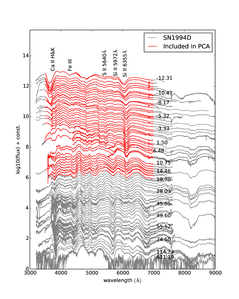
We limit the analysis in the 3500-7000 Å range. This is the wavelength range that is mostly complete in the data that we are using. We consider only spectra from $-12.5$ up to $+17.5$ days relative to $B$-maximum. Spectral observations become scarce outside of this epoch range. This fraction of the spectral variability of SNe Ia is highligted in Fig. 1 on the spectral series of SN 1994D, a prototypical SN Ia. The derivative spectra in the considered range of epochs are binned by time bins of $2.5$ days. The input matrix of the analysis has a number of columns equal to the number of wavelength bins times the number of epoch bins, and a number of rows equal to the number of SNe. Following Sasdelli et al. (2015), we apply EMPCA on this matrix to reduce the dimensionality of the data down to 5 principal components (PCs).

3.2 Interpolating the photometry with Gaussian Processes

For the Partial Least Square algorithm, we need to transform the discrete time series of the photometry into a continuous function. We need light curves as a continuous quantity with associated errors. These errors have to take into account the uncertainty of the observed photometry and the sparsity of the data. We need a robust regression method to fit light curves and color curves.

SN Ia photometry is typically interpolated with the help of light curve fitters. These algorithms construct a parametrized template for SN Ia light curve. When fitting only $B$ and $V$ bands, they usually employ only two parameters (e.g. SALT2 Guy et al., 2007). The first parameter accounts for the decline rate of the SN (e.g. $\Delta m_{15}(B)$or stretch), the second parameter accounts for a color correction using the observed color. This implicitly assumes that SN Ia light curves are described by two parameters only. This is, of course, true only as a first approximation, and from only the light curves it is hard to extract many more parameters. But from the study of the spectra (Benetti et al., 2005; Branch et al., 2006; Hachinger et al., 2006; Blondin et al., 2012) it is clear that SN Ia are much more diverse, and we want to take this diversity into account. For these reasons we do not want to use typical SN light curve fitters. With these fitters the result of the fit depends not only on the data of the SN under consideration, but also on the rest of the sample. Of course this makes sense if the aim is to calibrate the objects as well as possible, but it is not the best approach if we want to study the relations between light curves and spectra in an unbiased way.

A simple approach could be to obtain the light curves with the least square fit to a polynomial. This introduces biases in the result. Arbitrary choices such as the degree of the polynomial will affect the outcome. A better approach is the use of a spline fit. This is equivalent to using a series of polynomials smoothly connected together, but also this approach is inadequate for our purposes because it does not give a time dependent uncertainty on the result of the fit.

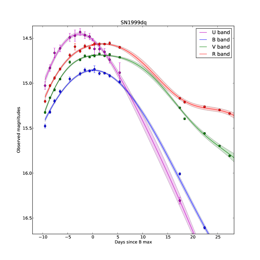
We use a powerful regression method based on Gaussian Processes (Rasmussen & Williams, 2005; Shafieloo et al., 2012; Kim et al., 2013). Gaussian Processes Regression is a more general approach to determine the underlining function from a sparse set of data (Appendix A). As an example, the result of Gaussian Process Regression on the photometry of the SN 1999dq is shown in Fig. 2. Now we have robust interpolated luminosities with sensible error estimates for the fitted light curves. Most importantly, the fits are independent from the behaviour of the other SNe of the sample.

Figure 2: Light curve fitting in four bands of the SN 1999dq. The fit is the result of a Gaussian Processes regression.

3.3 Multivariate Partial Least Square

We want to predict the light curves of SNe Ia from the PC space on the time series of spectra. A good tool for this job is Partial Least Square regression (Wold et al., 2001). Sasdelli et al. (2015) use univariate PLS, here we use the multivariate version of this regression technique.

The goal of PLS regression is to predict the $\mathcal{Y}$ space of the responses from the $\mathcal{X}$ space of the predictors to recover their common structure. PLS finds the linear relations that allow to predict a set of quantities in the $\mathcal{Y}$ space, called responses, from the space of predictors $\mathcal{X}$. The underlying assumption is that every component of the space of responses is a linear combination of the predictors. Mathematically the relation can be written as:

$$\textsf{{X}}=\textsf{{T}}\textsf{{P}}^{T}+residuals$$ (1)

$$\textsf{{Y}}=\textsf{{U}}\textsf{{Q}}^{T}+residuals$$

where X is the training set of predictors. X has dimensions $N\times M$ where $N$ is the number of observations (the number of SNe) and $M$ is the dimension of the predictor space $\mathcal{X}$. In our case $M$ is the dimension of the PCA space built from spectra. The matrix Y is the matrix of the training set of responses. It has dimensions $N\times L$ where $L$ is the number of epochs sampled from the light curve. T and U have dimensions $M\times n$ where $n$ is the dimensionality reduction of PLS, that is the number of components chosen to explain the relation between the space $\mathcal{X}$ and the space $\mathcal{Y}$. P and Q are called loadings. The decomposition is made so as to maximize the covariance between P and Q. The loadings become good summaries of the spaces $\mathcal{X}$ and $\mathcal{Y}$ and the residuals become “small”. T represents the projections on the latent structures defined by the matrix of the weights W:

$$\textsf{{T}}=\textsf{{W}}\textsf{{X}}.$$ (2)

The scores (T and U) have the property that they reproduce well X and Y, and the x-scores (T) are good predictors of Y:

$$\textsf{{Y}}=\textsf{{T}}\textsf{{Q}}^{T}+residuals,$$ (3)

when the residuals of the prediction have to be small.

The relation between the two spaces is best explained in Fig. 1 in Wold et al. (2001). The dimensionality of the initial space gets reduced to $n$, the dimension of the space of the latent variables, by the matrix W (equation 2). Then, the matrix T is responsible for predicting the space $\mathcal{Y}$ trough equation 3. In our case, the “structure descriptors” are the spectral series and the “activity measures” are the light curves. The variables are the coefficients of the PCA space of the spectra, the observations are the different SNe, {t₁, t₂, t₃} are the latent variables, Y is the matrix of the observed light curves, M is the dimension of the range of epochs included in the light curves.

Multivariate PLS is particularly recommended when there is a high correlation between the responses. This is the case for the magnitudes at different epochs of light curves and color curves.

The decompositions of X and Y are chosen to explain as much as possible of the covariance between the two datasets.

A simple algorithm to compute the weight matrix (W) and the scores (T and U) proceeds as shown in Algorithm 1. This algorithm is implemented in scikit-learn (Pedregosa et al., 2011).

The tools described before were made publicly available in the LC_predictor Python package. The code takes as input the series of spectra of a SN Ia and automatically performs the smoothing, and it projects the data on the trained PCA and PLS spaces. It outputs the reconstructed spectral series as a sanity check, and it produces the predicted light curves and color curves after reddening corrections.

Algorithm 1 Partial Least Square algorithm

1. Assign $\textsf{{X}}_{0}=\textsf{{X}}$ and $\textsf{{Y}}_{0}=Y$ (first iteration)

2. repeat $n$ times (the chosen dimensionality reduction)

   Compute the Singular Value Decomposition (SVD) of the matrix $\textsf{{X}}_{n}^{T}\textsf{{Y}}_{n}$

   Compute the first left singular vector ($w_{n}$) of the matrix $\textsf{{X}}_{n}^{T}Y_{n}$.

   Compute the first right singular vectors ($v_{n}$) of the matrix $\textsf{{X}}_{n}^{T}\textsf{{Y}}_{n}$.

   Compute the $n$th X-score: $T_{n}$ = $\textsf{{X}}_{n}w_{n}$

   Compute the $n$th Y-score: $U_{n}$ = $\textsf{{Y}}_{n}v_{n}$

   Deflate the X matrix: $\textsf{{X}}_{n}+1$ = $\textsf{{X}}_{n}-T_{n}P_{n}^{T}$. It is not necessary to deflate Y.

4 Predicting Light Curves and Color Curves from the Spectra

In this section we use multivariate PLS regression to find correlations between photometry and spectral properties. The spectral properties are described by the coefficients of the PCA space constructed from spectral series. The coefficients from the PCA encode the variance within Type Ia SNe spectral series in 5 components. The good quality of the reconstructions of the spectra prove that this decomposition encompasses the variability of Type Ia spectra. This space, by construction, does not include reddening.

The intrinsic colors and absolute magnitudes are a function of the spectral series. Physically, a given spectral series is expected to have a corresponding intrinsic color curve and light curve. That is, the luminosity and color at a certain epoch are expected to be a function of the components of the PCA space constructed from the spectra. We use PLS regression to extract this function. Using this approach, we make the implicit assumption of linearity. That is, the intrinsic colors and absolute magnitudes are assumed to be well approximated by linear functions of the components of the PCA space of the spectra.

The observed colors are subject to reddening. To find the intrinsic color one has to find the locus of the bluest SN for every point of the PCA space. We use an approach similar to what was used by Sasdelli et al. (2015) to discard SNe with large reddening. In that case we had only one parameter for the treshold of maximum reddening to select the SNe, here we have more complicated color curves and light curves. Additionally, we are using photometric data that have a larger diversity in their errors. We select supernovae for the PLS regression if they have a reddening lower than a given treshold above the PLS prediction and with errors lower than a given value in all the epochs. The PLS algorithm and the selection is run a number of times until the solution has converged (see section 5.4 of Sasdelli et al., 2015). The supernovae in each iteration can be selected or deselected. These parameters are validated through cross-validation.

4.1 Predicting the Light Curve from the Spectra

We apply the approach to the $B$-band light curves between $-5$ days and $+35$ days from maximum. The aim is to predict the absolute magnitude curve using the spectra of the supernova. This is done free from assumptions on reddening laws and extinction. First of all the observed magnitudes need to be scaled to the reference frame. This is simply achieved using the host-galaxy redshift and assuming a smooth Hubble flow. The observed magnitude needs to be decreased by the distance modulus:

$$\text{M}_{abs}=\text{M}_{obs}-\mu$$

where, assuming an homologous expansion for the Hubble flow:

$$\mu=5(\log_{10}(zc/H{{}_{0}})+5).$$

The peculiar motion of the galaxies will add an error to this estimate. The error on the absolute magnitudes due to the dispersion of the peculiar velocity $\sigma(v)$ of the galaxies becomes:

$$\sigma_{\mu}=5\sigma(v)/(\ln(10)zc).$$

Figure 3: the left and the right panel represent the space of predictors and the space of responses and correspond to the X and Y spaces of section 3.3. The left panel shows the spectra close to B maximum of some SNe examples. The fluxes are in arbitrary units and the spectra have been shifted for clarity. The right panel shows the photometry of the same SNe. The solid curves are the predictions based on PLS regression on the PCA space on the spectra. The blue dashed curve show the effect of adding extinction on the predicted light curve of the SN 1995E.

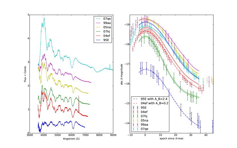
The left panel of Fig. 3 shows, as an example, the spectra of a few SNe close to maximum brightness. The significant variability in spectral properties present in the data is apparent from this selection. In the right panel we show the corresponding light curves of these SNe. The points are the original photometry, corrected for Hubble flow, but with no attempts to correct for reddening. The solid curves show the corresponding PLS predictions. The colored area represents the uncertainty of the prediction calculated using k-folding. The photometric data and the predictions match nicely. SN 1995E, however, has a luminosity significantly lower than is predicted. This is expected and it can be explained by a significant amount of reddening of this individual object. As it was shown in Sasdelli et al. (2015), reddening does not influence the components of the PCA space. Consequently, a supernova with high reddening does not have a PLS prediction different from a supernova with no reddening. From this we deduce that the mismatch between the prediction and the observations comes from dust extinction. On individual objects the mismatch can be slightly negative. However, these mismatches are always consistent with zero, i.e. no reddening. This is due to random uncertainties in the observed data, in the distance estimates and in the analysis.

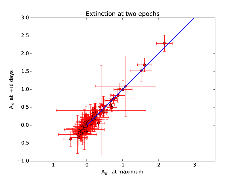
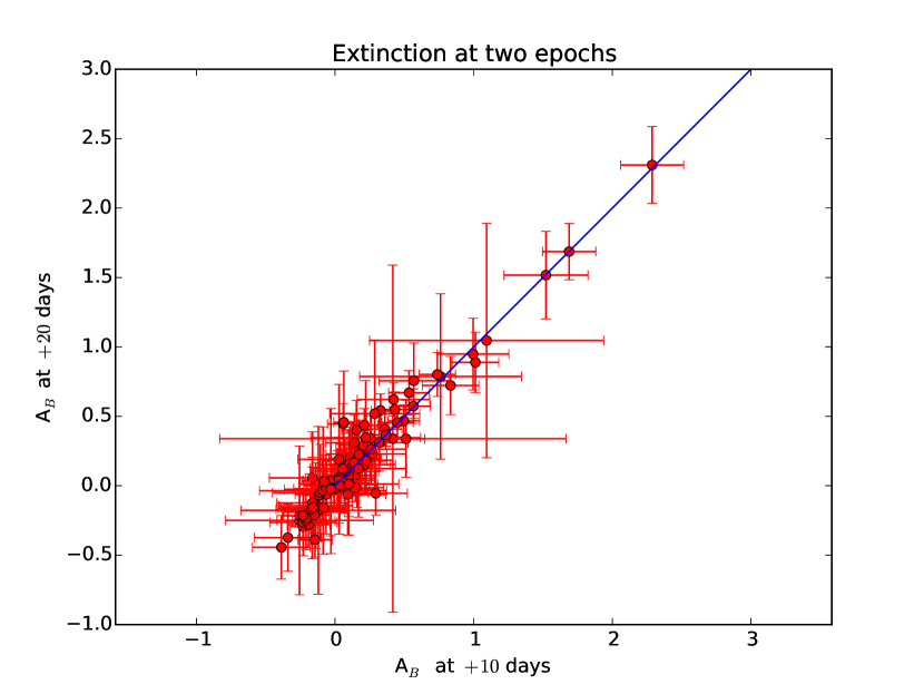
The difference between the curve and the data is an estimate of the extinction independent from assumptions on the nature of the reddening law or the amount of reddening. Clearly, this estimate can be calculated at different epochs. Under the assumption that the amount of extinction does not vary with time, the luminosity deficit of a supernova in a given band as a first order approximation stays constant. We check it in Fig. 4. It shows the extinction in the $B$ band (A_B) at maximum and at $+10$ days for all the supernovae in our sample. Fig. 5 shows the extinction in the $B$ band at $+10$ days and at $+20$ days. The extinctions are consistent between each other, which implies that the extinction does not vary significantly after maximum, and supports the reliability of our method.

Figure 4: The figure shows the A_B at maximum and at $+10$ days obtained by PLS regression. The solid line is not a fit. It is just a diagonal overplotted as a reference.

Figure 5: The figure shows the A_B at $+10$ days and at $+20$ days obtained by PLS regression.

4.2 The Phillips-Relation

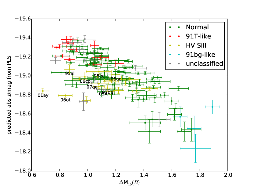
Type Ia SNe luminosity is known to anti-correlate with the decline in luminosity after maximum (Phillips, 1993). From the PLS regression we have an estimate for the $B$-band peak luminosity independent from reddening assumptions. In Fig. 6 we show the relation between our estimate and the $\Delta m_{15}(B)$, the difference between the magnitude at maximum and at $+15$ days. Many of the known characteristics of SN Ia show up in this diagram. On the bottom right are the faint and fast declining 1991bg-like SNe. There are only a few objects of that kind in our sample, hence the errors on the predicted magnitudes are large. Spectroscopically normal SNe show a wide range of luminosities and decline rates. On the tip of the relation are the luminous 1991T-like SNe. An interesting “outlier” of the Phillips relationship is the SN 2001ay. It is the left-most point in the figure, with a $\Delta m_{15}(B)$= 0.7 (the slowest of the sample). This SN is so extreme that is was clearly recognized as an outlier of the relation by Krisciunas et al. (2011). It is too faint for its decline rate. Our analysis nicely confirms it and shows that such outliers (although less extreme) are not uncommon. This suggests that there is a population of SNe with characteristics that are intermediate between SN 2001ay and the bulk of SNe Ia. These SNe are highlited in Fig. 6. They can be roughly identified with the SNe Ia with a high photospheric velocities in their lines (HV in the classification scheme from Wang et al., 2009). Many of these SNe are “underluminous” compared to what their $\Delta m_{15}(B)$ predicts. Most of these SNe are characterized by high photospheric velocities and intrinsically redder colors than the average.

Figure 6: The Phillips relationship between the $B$-band luminosity at maximum predicted by PLS and the decline rate of the light curve. The different subclasses of SN Ia are colored (Li et al., 2001; Wang et al., 2009). The SNe that are close to SN 2001ay in the PCA space are tagged.

4.3 Predicting the Color Curve from the Spectra

In this section we apply the PLS regression method on $B-V$ color curves. Differently from magnitudes, the observed colors are not affected by the distance, and can usually be measured precisely in nearby SNe. However, the intrinsic variance of colors is smaller than the variance in the magnitudes. This makes the regression task quite complicated.

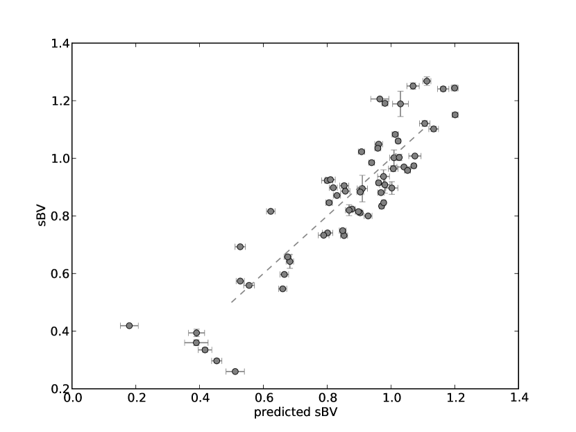
First, we want to show that important characteristics of the $B-V$ color curve are retained in the PCA space of spectra. The time between the $B$ maximum epoch and the maximum in the $B-V$ color curve is an almost reddening independent quantity. Its use was suggested for SN Ia classification and cosmology (Burns et al., 2014) as an alternative to $\Delta m_{15}(B)$. The maximum in the $B-V$ color curve happens usually at about $+30$ days after maximum. This quantity is shown to correlate with the spectral properties encoded in our PCA space. Simple univariate PLS regression between the PCA space and this color curve indicator shows an excellent correlation (Fig. 7).

Figure 7: The relation between the epoch of the $B-V$ maximum in units of $30$ days (s_BV, Burns et al., 2014) and its prediction from PLS regression performed on the PCA space of spectral properties.

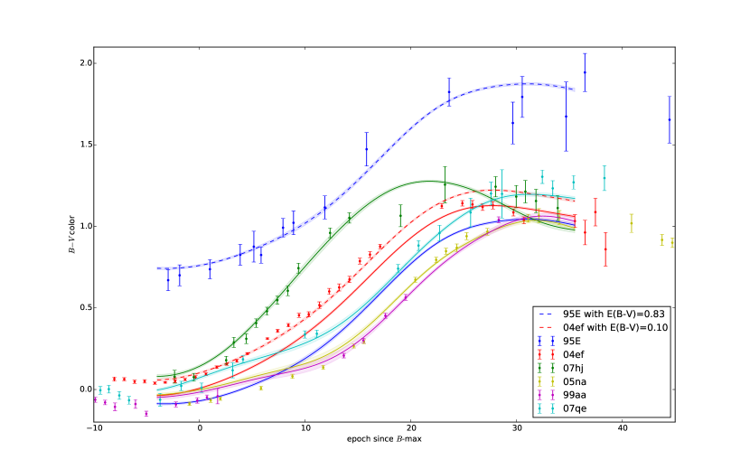
Sasdelli et al. (2015) also showed that the color at maximum has a significant correlation with spectral properties. Here we generalize these individual approaches with the help of multivariate PLS. Fig. 8 shows some observed color curves (points with errorbars) and the corresponding predictions from the spectra using PLS (solid lines). The left panel of Fig. 3 shows the spectra of the corresponding SNe at maximum. It is evident that the colors are quite uniform at maximum, later they have a large spread of properties. SN 1995E has clearly a significant color excess in comparison with the prediction from its spectra. This is consistent with a significant amount of reddening. The analysis converts the spectral variability present in the spectra into a prediction for the intrinsic color curve (solid curve).

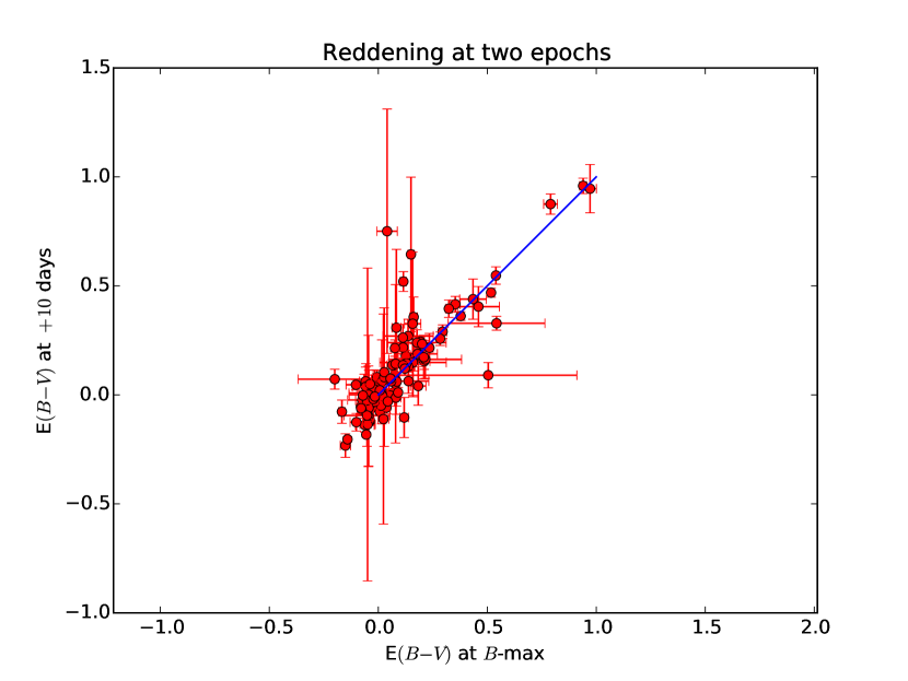
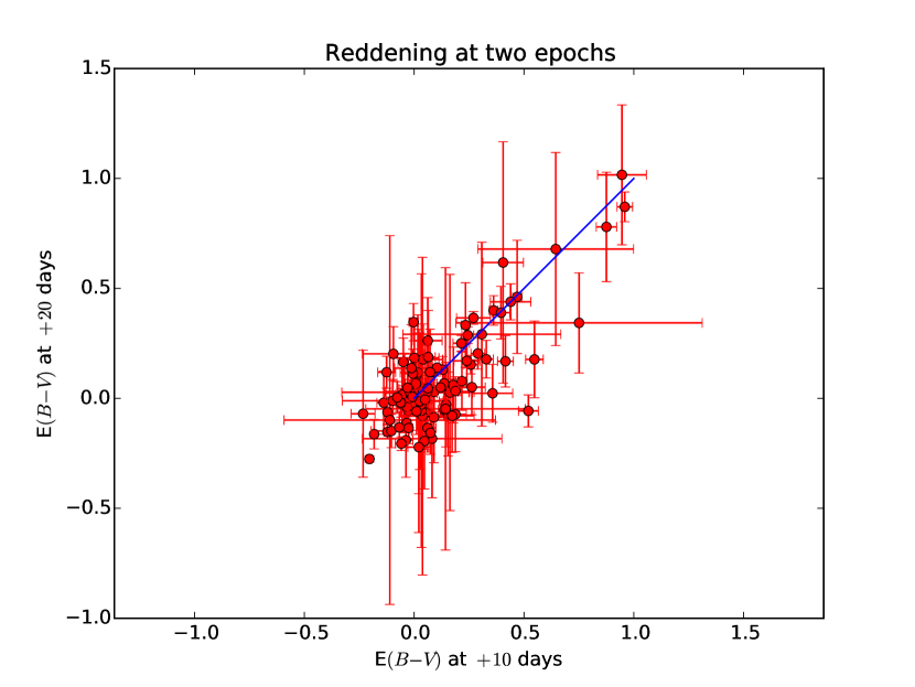
Similarly to before, we want to check that the PLS regression is predicting most of the intrinsic color variability. Under the assumption that the amount of reddening does not vary significantly with time, we check that the color excess attributed to dust is constant at different epochs. Figs. 9 and 10 compare the color excess at maximum, at $+10$ and at $+20$ days. The agreement between the quantities supports that the regression predicts the majority of the intrinsic color variation and evolution and that the amount of reddening does not change significantly in this range of epochs.

Figure 8: The figure shows the observed $B-V$ colors for a number of SNe (dots with errorbars). These are compared with the color curves predicted from the spectra by means of PLS regression (solid lines). The blue dashed curve shows the effect of adding extinction on the predicted color curve of the extinguished SN 1995E.

Figure 9: The figure shows the $E(B-V)$ predicted by mulivariate PLS regression at maximum and at $+10$ days. A diagonal is overplotted as a reference.

Figure 10: The figure shows the $E(B-V)$ predicted by mulivariate PLS regression at $+10$ and at $+20$ days.

4.4 The Extinction-Reddening Relation

The extinction due to dust affects most short wavelengths. This means that the dimming in the $B$ band (A_B) will be larger than the effect in the $V$ band. Hence, the relation between the extinction in these bands is usually parametrized as:

$$A_{V}=R_{V}E(B-V).$$

Typical values for $R_{V}$ measured in our galaxy vary between $2.1$ and $5.8$ with $3.1$ being the most common value (Cardelli et al., 1989; Draine, 2003).

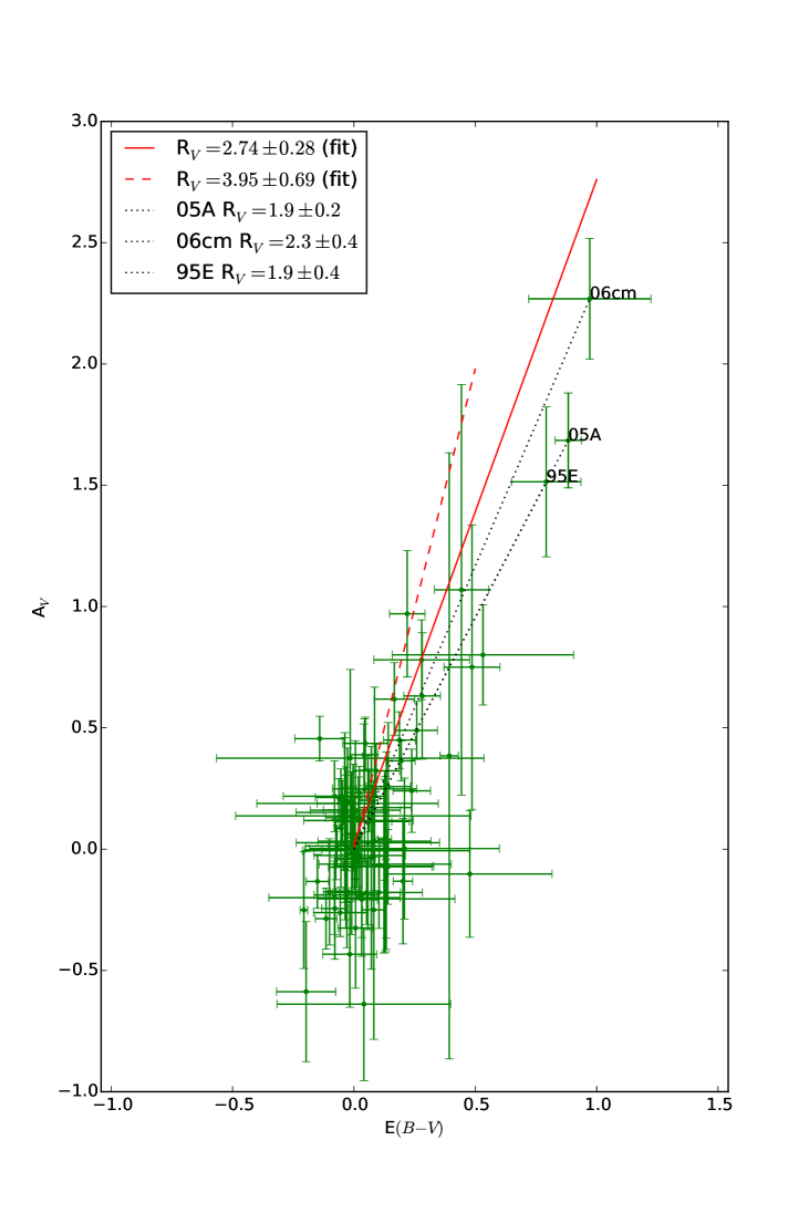
Fig. 11 shows the color and magnitudes excess from the PLS reconstruction. Frequently SN Ia are associated with a low $R_{V}$ (frequently $<2$) that does not show up in galactic reddening (e.g. Conley et al., 2007; Mandel et al., 2011; Burns et al., 2014). This have been explained by peculiar environments around SN Ia (e.g. Goobar, 2008; Foley et al., 2014). In contrast, techniques based on spectral features return values of $R_{V}$ much more similar to what is typical in the Milky Way (Chotard et al., 2011). Assuming that a significant fraction of the residuals in the Hubble diagram is due to intrinsic color instead of the intrinsic luminosity also favours a Milky-Way R_V (Scolnic et al., 2014). Performing an orthogonal distance regression fit on the results of our analysis returns an $R_{V}=2.78\pm 0.28$ (Fig. 11). This shows that the average host extinction of SNe Ia is consistent with the typical extinction laws of the Milky-Way (R${}_{V}=3.1$). In Fig. 11 we also perform a fit excluding the three most extinguished SNe of our sample. This confirms what was found by Folatelli et al. (2010). SNe with an high extinction often have low values of $R_{V}$ (Fig. 11), and SNe with a low extinction show an average R_V similar to typical Milky Way values (dashed line).

It is hard to discriminate between spectroscopically different SNe by using only light curves. Certain spectral types (mostly SNe with high photospheric velocities) have light curve and color curve shapes similar to average SN Ia but fainter and redder. Techniques of color-curve matching may find a match between two SNe that are intrinsically different and think that differences that are intrinsic dome from dust extinction. The ratio between this “missing luminosity” and “color excess” happens to be significantly lower than what is due to typical dust. If their spectral characteristics are not taken into account, the light curves and color curves of spectroscopically different SNe will be compared like they are coming from a similar object and lead to low estimates for the average $R_{V}$ of SNe Ia. An illuminating example of this degeneracy between intrinsic color and dust-extinction that can be broken using the spectra is shown by the slow-declining SN 2007qe ($\Delta m_{15}(B)$$=0.98\pm 0.05$, Hicken et al., 2009). This SN is approximately as slow declining as the bright SN 1999aa ($\Delta m_{15}(B)$$=0.85\pm 0.05$, Jha et al., 2006). The two light curves are very similar if they are shifted in order to match (Fig. 3). This degeneracy is not broken using extensive $B-V$ color curve observations. Fig. 8 shows how the two $B-V$ color curves are similar. The only difference is a constant shift that is easy to misjudge as reddening. Looking at the spectra, however, the strong differences between the two SNe are immediately apparent. The equivalent widths of corresponding lines are significantly different, and the velocity of the lines in the two spectra are extremely different. SN 2007qe has a larger velocity and is redder (in agreement with Foley et al. (2011)). Without the availability of spectroscopic information, the ratio between the color “excess” of SN 2007qe and SN 1999aa and the difference in luminosity would mimic an extinction with a low $1.<R_{V}<1.5$. This is just an extreme example, and there are many other SNe that are intermediate cases. All these intermediate cases may introduce a shift to the average $R_{V}$. Scolnic et al. (2014) showed that having uncertainty in the determination of the intrinsic color can favour low $R_{V}$ values. Using the spectral information, we show that such a dispersion, not accounted by looking only at light curves, is present in the data.

This degeneracy in the light and color curve spaces may be also broken by using properly good $U$ band photometry. In the $U$ band the effect of dust is the strongest, and from most studies based on color-curve matching it is clear that there is a significant amount of residual intrinsic scatter in this band (e.g Burns et al., 2014). For example, with pre-maximum U band photometry it may be possible to discriminate between SN 1999aa and SN 2007qe. SN 1999aa has a bright and early peak in the $U$-band that is not present in SN 2007qe. However, it may still not be enough to separate intrinsic color from extinction as much as using spectral information for all SNe Ia.

The presence of circumstellar dust was proved in a few higly extinguished SNe Ia (e.g. Patat et al., 2007). Part of the extinction in some SNe Ia has to come from circumstellar dust. If this circumstellar dust is close enough to the SN, multiple scattering produces an extinction with a low $R_{V}$ (Goobar, 2008). This can be the source of a low $R_{V}$ for few highly extinguished SNe. From a physical point of view, our finding of a normal $R_{V}$ for most SNe Ia means that the dust in front of the majority of them is quite normal. This suggests that the majority of SN Ia extinction is caused by simple interstellar dust in the host galaxy and it is not related to the progenitor of the SN.

Figure 11: The plot shows the relation between the host-galaxy extinction in $V$ and reddening in $B-V$. The solid line shows the result of a fit of the relation. The dashed line shows the fit excluding the three most reddened SNe, for which an individual estimate of $R_{V}$ is calculated. The errors come from the measurement errors and from statistical errors (k-folding) added in quadrature.

5 Conclusions

We build on the physically motivated assumption that the intrinsic light curve and color curve variability are a function of the variability in spectral series.

In the context of SN Ia, multivariate PLS, together with PCA, becomes a sharp tool able to separate the intrinsic variability and the variability due to dust. This approach can be valuable in a number of challenges, such as the study of the reddening law and its possible variability and improving the calibration of SNe Ia luminosity by the use of their spectra which have plenty of distance-independent properties. In this work we investigate the $R_{V}$ dust parameter, the most commonly used parameter to characterize the type of dust. Our results suggest a solution for the tension between the range of observed values for this parameter in the Milky-Way and the values sometimes inferred from SNe Ia. We find that the majority of the host galaxy extinction of SNe Ia is caused by normal dust, similar to the typical Milky-Way dust. This suggests that most of the dust associated with SNe Ia is of interstellar origin and not associated with the progenitor.

Our technique allows to predict the absolute magnitude of SNe Ia without assuming the decline rate luminosity relation. This permits to test this relation without assumptions on the reddening, that depends on how the intrinsic color of the SN is estimated. The technique can have a number of cosmological applications. Used together with the traditional light curve fitting, our approach may lead to a better relative calibration of SNe Ia with a good spectral coverage. This can be particularly useful to set the relative calibration between the few SNe Ia with a reliable Cepheid distance measurement and the SNe Ia in the smooth Hubble-Flow.

The modelling of SNe Ia by means of radiation transport techniques (e.g. Stehle et al., 2005) requires precise measurements of the distance and of the amount of extinction of the selected SN. Traditional methods have often large uncertainties on the distance of nearby galaxies and on the host galaxy reddening. Although the distance of the SN and its intrinsic color can be obtained directly from the modelling (Sasdelli et al., 2014), this procedure is time consuming and introduces new free parameters. The method described in our work gives estimates for the absolute magnitude and the intrinsic color for most common spectral types of SNe Ia. This can be used to speed up their modelling and reduce the number of free parameters involved. It will also help in keeping the consistency of the luminosity and color between the models of distinct SNe.

Our study shows how important is to obtain spectral coverage for the study of SNe Ia, not only for the study of peculiar objects, but also for the study of typical SNe Ia. Incoming automated surveys such as Pan-STARRS and the Large Synoptic Survey Telescope (LSST) will produce large amount of light curves without accompanying spectra. This study suggests investing significant fraction of available telescope time and resourses in studying spectroscopy. This also suggests that detailed planning of the limited spectroscopic follow-up available could optimize the color and extinction estimation of the entire photometric sample.

Our approach can easily be extended to other colors and magnitudes in a broader wavelength range. This will be investigated in detail in future work.

Appendix A Gaussian Processes

The technique assumes that the data are distributed with a Gaussian distribution with infinite dimensionality. In every epoch the outcome of a measurement is assumed to follow a Gaussian distribution. Our set of n photometric measurements can be seen as one realization of an n-variate Gaussian distribution in an n-dimensional space. Now, two epochs close to each other are expected to be correlated. That is, the luminosity of our SN does not change much in a day. Two observations at different epochs are related by a covariance function, $k(t_{0},t_{1})$, that encodes the relation between the magnitudes at $f(t_{0})$ and $f(t_{1})$. A safe assumption for the structure of this covariance is:

$$k(t_{i},t_{j})=\sigma_{f}^{2}\exp\left[-\frac{(t_{i}-t_{j})^{2}}{2\tau^{2}}\right]+\sigma_{n}^{2}\delta_{ij}$$ (4)

The first term means that the correlation is high for observations distant by less than $\sim\tau$ and negligible when the time difference is larger, the second term accounts for the noise. Without noise in the data the correlation between two realizations temporally very close would be as high as the covariance of an individual realization. Adding noise, the covariance of a given measurement is larger by $\sigma_{n}^{2}$. In practice, these coefficients parametrize how slowly the underling function varies with time $(\tau)$, how big the total standard deviation of the magnitudes $(\sigma_{f})$ is, and how much uncertainty is due to the noise of the individual measurements $(\sigma_{n})$. $\sigma_{f},\sigma_{n}$, and $\tau$ are called hyperparameters of the model. For a given set of hyperparameters, it is possible to produce a large number of realizations that are likely to reproduce the observations. The average and the standard deviation of these realizations will look like the fits in Figure 2. The quality of the fit, however, will heavily depend on the choices of the hyperparameters of equation 4. For example, if $\sigma_{n}$ is set to zero the fit will lie exactly on the photometry overfitting the data. On the other hand, too large a $\tau$ will remove small scale variations from the fit, flattening the peaks. The optimal hyperparameters are not chosen by hand but are retrieved by a maximization of the probability $p(\{\sigma_{f},\sigma_{n},\tau\}|obs)$ of having a certain set of hyperparameters for the given observations.

References

- Benetti et al. (2005) Benetti S. et al., 2005, ApJ, 623, 1011
- Blondin et al. (2012) Blondin S. et al., 2012, AJ, 143, 126
- Branch et al. (2006) Branch D. et al., 2006, PASP, 118, 560
- Burns et al. (2014) Burns C. R. et al., 2014, ApJ, 789, 32
- Cardelli et al. (1989) Cardelli J. A., Clayton G. C., Mathis J. S., 1989, ApJ, 345, 245
- Chotard et al. (2011) Chotard N. et al., 2011, A&A, 529, L4
- Conley et al. (2007) Conley A., Carlberg R. G., Guy J., Howell D. A., Jha S., Riess A. G., Sullivan M., 2007, ApJ, 664, L13
- Draine (2003) Draine B. T., 2003, ARA&A, 41, 241
- Folatelli et al. (2013) Folatelli G. et al., 2013, ApJ, 773, 53
- Folatelli et al. (2010) Folatelli G. et al., 2010, AJ, 139, 120
- Foley et al. (2014) Foley R. J. et al., 2014, MNRAS, 443, 2887
- Foley & Kasen (2011) Foley R. J., Kasen D., 2011, ApJ, 729, 55
- Foley et al. (2011) Foley R. J., Sanders N. E., Kirshner R. P., 2011, ApJ, 742, 89
- Ganeshalingam et al. (2010) Ganeshalingam M. et al., 2010, ApJS, 190, 418
- Goobar (2008) Goobar A., 2008, ApJ, 686, L103
- Guy et al. (2007) Guy J. et al., 2007, A&A, 466, 11
- Hachinger et al. (2006) Hachinger S., Mazzali P. A., Benetti S., 2006, MNRAS, 370, 299
- Hawkins et al. (2003) Hawkins E. et al., 2003, MNRAS, 346, 78
- Hicken et al. (2009) Hicken M. et al., 2009, ApJ, 700, 331
- Hogg et al. (2002) Hogg D. W., Baldry I. K., Blanton M. R., Eisenstein D. J., 2002, ArXiv Astrophysics e-prints
- Jha et al. (2006) Jha S. et al., 2006, AJ, 131, 527
- Kim et al. (2013) Kim A. G. et al., 2013, ApJ, 766, 84
- Krisciunas et al. (2011) Krisciunas K. et al., 2011, AJ, 142, 74
- Li et al. (2001) Li W., Filippenko A. V., Treffers R. R., Riess A. G., Hu J., Qiu Y., 2001, ApJ, 546, 734
- Mandel et al. (2014) Mandel K. S., Foley R. J., Kirshner R. P., 2014, ApJ, 797, 75
- Mandel et al. (2011) Mandel K. S., Narayan G., Kirshner R. P., 2011, ApJ, 731, 120
- Mazzali et al. (2014) Mazzali P. A. et al., 2014, MNRAS, 439, 1959
- Nordin et al. (2011) Nordin J. et al., 2011, ApJ, 734, 42
- Oke & Sandage (1968) Oke J. B., Sandage A., 1968, ApJ, 154, 21
- Patat et al. (2007) Patat F. et al., 2007, Science, 317, 924
- Pedregosa et al. (2011) Pedregosa F. et al., 2011, Journal of Machine Learning Research, 12, 2825
- Perlmutter et al. (1999) Perlmutter S. et al., 1999, ApJ, 517, 565
- Phillips (1993) Phillips M. M., 1993, ApJ, 413, L105
- Phillips et al. (1999) Phillips M. M., Lira P., Suntzeff N. B., Schommer R. A., Hamuy M., Maza J., 1999, AJ, 118, 1766
- Rasmussen & Williams (2005) Rasmussen C. E., Williams C. K. I., 2005, Gaussian Processes for Machine Learning (Adaptive Computation and Machine Learning). The MIT Press
- Reindl et al. (2005) Reindl B., Tammann G. A., Sandage A., Saha A., 2005, ApJ, 624, 532
- Riess et al. (1998) Riess A. G. et al., 1998, AJ, 116, 1009
- Riess et al. (1996a) Riess A. G., Press W. H., Kirshner R. P., 1996a, ApJ, 473, 88
- Riess et al. (1996b) Riess A. G., Press W. H., Kirshner R. P., 1996b, ApJ, 473, 588
- Sasdelli et al. (2015) Sasdelli M. et al., 2015, MNRAS, 447, 1247
- Sasdelli et al. (2014) Sasdelli M., Mazzali P. A., Pian E., Nomoto K., Hachinger S., Cappellaro E., Benetti S., 2014, MNRAS, 445, 711
- Schlafly & Finkbeiner (2011) Schlafly E. F., Finkbeiner D. P., 2011, ApJ, 737, 103
- Schlegel et al. (1998) Schlegel D. J., Finkbeiner D. P., Davis M., 1998, ApJ, 500, 525
- Scolnic et al. (2014) Scolnic D. M., Riess A. G., Foley R. J., Rest A., Rodney S. A., Brout D. J., Jones D. O., 2014, ApJ, 780, 37
- Shafieloo et al. (2012) Shafieloo A., Kim A. G., Linder E. V., 2012, Phys. Rev. D, 85, 123530
- Silverman et al. (2012) Silverman J. M. et al., 2012, MNRAS, 425, 1789
- Stehle et al. (2005) Stehle M., Mazzali P. A., Benetti S., Hillebrandt W., 2005, MNRAS, 360, 1231
- Stritzinger et al. (2011) Stritzinger M. D. et al., 2011, AJ, 142, 156
- Wang et al. (2009) Wang X. et al., 2009, ApJ, 699, L139
- Wold et al. (2001) Wold S., Sjöström M., Eriksson L., 2001, Chemometrics and intelligent laboratory systems, 58, 109
- Yaron & Gal-Yam (2012) Yaron O., Gal-Yam A., 2012, PASP, 124, 668