Long Term Effects of Small Random Perturbations on Dynamical Systems: Theoretical and Computational Tools

Abstract.

Small random perturbations may have a dramatic impact on the long time evolution of dynamical systems, and large deviation theory is often the right theoretical framework to understand these effects. At the core of the theory lies the minimization of an action functional, which in many cases of interest has to be computed by numerical means. Here we review the theoretical and computational aspects behind these calculations, and propose an algorithm that simplifies the geometric minimum action method to minimize the action in the space of arc-length parametrized curves. We then illustrate this algorithm’s capabilities by applying it to various examples from material sciences, fluid dynamics, atmosphere/ocean sciences, and reaction kinetics. In terms of models, these examples involve stochastic (ordinary or partial) differential equations with multiplicative or degenerate noise, Markov jump processes, and systems with fast and slow degrees of freedom, which all violate detailed balance, so that simpler computational methods are not applicable.

1. Introduction

Small random perturbations often have a lasting effect on the long-time evolution of dynamical systems. For example, they give rise to transitions between otherwise stable equilibria, a phenomenon referred to as metastability that is observed in a wide variety of contexts, e.g. phase separation, population dynamics, chemical reactions, climate regimes, neuroscience, or fluid dynamics. Since the time-scale over which these transition events occurs is typically exponentially large in some control parameter (for example the noise amplitude), a brute-force simulation approach to compute these events quickly becomes infeasible. Fortunately, it is possible to exploit the fact that the mechanism of these transitions is often predictable when the random perturbations have small amplitude: with high probability the transitions occur by their path of maximum likelihood (PML), and knowledge of this PML also permits to estimate their rate. This is the essence of large deviation theory (LDT) [20], which applies in a wide variety of contexts. For example, systems whose evolution is governed by a stochastic (ordinary or partial) differential equation driven by a small noise or by a Markov jump process in which jumps occur often but lead to small changes of the system state, or slow/fast systems in which the fast variables are randomly driven and the slow ones feel these perturbations through the effect fast variables only, all fit within the framework of LDT. Note that, typically, the dynamics of these systems fail to exhibit microscopic reversibility (detailed balance) and the transitions therefore occur out-of-equilibrium. Nevertheless, LDT still applies.

LDT also indicates that the PML is computable as the minimizer of a specific objective function (action): the large deviation rate function of the problem at hand. This is a non-trivial numerical optimization problem which calls for tailor-made techniques for its solution. Here we will focus on one such technique, the geometric minimum action method (gMAM, [39, 25, 39]), which builds the minimum action method and its variants [17, 44, 41], and was designed to perform the action minimization over both the transition path location and its duration. This computation gives the so-called quasipotential, whose role is key to understand the long time effect of the random perturbations on the system, including the mechanism of transitions events induced by these perturbations. Our purpose here is twofold. First, we would like to briefly review the theoretical aspects behind LDT that led to the rate function minimization problem and, in particular, to the geometric variant of it that is central in gMAM. Second, we would like to discuss in some details the computational issues this minimization entails, and remedy a drawback of gMAM, namely its somewhat complicated descent step that requires higher order derivatives of the large deviation Hamiltonian. Here, we propose a simpler algorithm, minimizing the geometric action functional, but requiring only first order derivatives of the Hamiltonian. The power of this algorithm is then illustrated via applications to a selection of problems:

1. the Maier-Stein model, which is a toy non-gradient stochastic ordinary differential equation that breaks detailed balance;

2. a stochastic Allen-Cahn/Cahn-Hilliard partial differential equation motivated by population dynamics;

3. the stochastic Burgers-Huxley PDE, related to fluid dynamics and neuroscience;

4. Egger’s and Charney-DeVore equations, introduced as climate models displaying noise-induced transitions between metastable regimes;

5. a generalized voter/Ising model with multiplicative noise;

6. metastable networks of chemical reaction equations and reaction-diffusion equations;

7. a fast/slow system displaying transitions of the slow variables induced by the effects of the fast ones.

The remainder of this paper is organized as follows. In Sect. 2 we briefly review the key concepts of LDT that we will use (Sect. 2.1) and give a geometrical point of view of the theory that led to the action used in gMAM (sec. 2.2). In Sect. 3 we discuss the numerical aspects related to the minimization of the geometric action, propose a simplified algorithm to perform this calculation, and compare it to existing algorithms. We also discuss further simplifications of the algorithm that apply in regularly occurring special cases, such as additive or multiplicative Gaussian noise. Finally, in Sect. 4 we present the applications listed above.

2. Freidlin-Wentzell large deviation theory (LDT)

Here we first give a brief overview of LDT [20], focusing mainly on stochastic differential equations (SDEs) for simplicity, but indicating also how the theory can be extended to other models, such as Markov jump processes or fast/slow systems. Then we discuss the geometric reformulation of the action minimization problem that is used in gMAM.

2.1. Some key concepts in LDT

Consider the following SDE for $X\in\mathbb{R}^{n}$

(1) $$dX=b(X)dt+\sqrt{\epsilon}\sigma(X)dW\,,$$

where $b:\mathbb{R}^{n}\to\mathbb{R}^{n}$ denotes the drift term, $W$ is a standard Wiener process in $\mathbb{R}^{n}$, $\sigma:\mathbb{R}^{n}\to\mathbb{R}^{n}\times\mathbb{R}^{n}$ is related to the diffusion tensor via $a(x)=(\sigma\sigma^{\dagger})(x)$, and $\epsilon>0$ is a parameter measuring the noise amplitude. Suppose that we want to estimate the probability of an event, such as finding the solution in a set $B\subset\mathbb{R}^{n}$ at time $T$ given that it started at $X(0)=x$ at time $t=0$. LDT indicates that, in the limit as $\epsilon\to 0$, this probability can be estimated via a minimization problem:

(2) $$\mathbb{P}^{x}\left(X(T)\in B\right)\asymp\exp\left(-\epsilon^{-1}\min_{\phi\in\mathcal{C}}S_{T}(\phi)\right)\,.$$

Here $\asymp$ denotes log-asymptotic equivalence (i.e. the ratio of the logarithms of both sides tends to 1 as $\epsilon\to 0$), the minimum is taken over the set $\mathcal{C}=\{\phi\in C([0,T],\mathbb{R}^{n}):\phi(0)=x,\phi(T)\in B\}$, and we defined the action functional

(3) $$S_{T}(\phi)=\begin{cases}\int_{0}^{T}L(\phi,\dot{\phi})\,dt&\text{if the integral converges}\\ \infty&\text{otherwise.}\end{cases}$$

Here

(4) $$L(\phi,\dot{\phi})=\tfrac{1}{2}\langle\dot{\phi}-b(\phi),\left(a(\phi)\right)^{-1}(\dot{\phi}-b(\phi))\rangle\,,$$

where we assumed for simplicity that $a(\phi)$ is invertible – (this assumption will be relaxed below) and $\langle\cdot,\cdot\rangle$ denotes the Euclidean inner product in $\mathbb{R}^{n}$. LDT also indicates that, as $\epsilon\to 0$, when the event occurs, it does so with $X$ being arbitrarily close to the minimizer

(5) $$\phi_{*}=\mathop{\text{argmin }}_{\phi\in\mathcal{C}}S_{T}(\phi)$$

in the sense that

$$\forall\delta>0:\qquad\lim_{\epsilon\to 0}\mathbb{P}^{x}\Bigl{(}\,\sup_{0\leq t\leq T}|X(t)-\phi_{*}(t)\,|\,<\delta\Big{|}X(T)\in B\Bigr{)}=1$$

Thus, from a computational viewpoint, the main question becomes how to perform the minimization in (5). Note that, if we define the Hamiltonian associated with the Lagrangian (4)

(6) $$H(\phi,\theta)=\langle b(\phi),\theta\rangle+\tfrac{1}{2}\langle\theta,a(\phi)\theta\rangle$$

such that

(7) $$L(\phi,\dot{\phi})=\sup_{\theta}\left(\langle\dot{\phi},\theta\rangle-H(\phi,\theta)\right),$$

this minimization reduces to the solution of Hamilton’s equations of motion,

(8) $$\begin{cases}\dot{\phi}=H_{\theta}(\phi,\theta)=b(\phi)+a(\phi)\theta\\ \dot{\theta}=-H_{\phi}(\phi,\theta)=-(b_{\phi}(\phi))^{T}\theta+\tfrac{1}{2}\langle\theta,a_{\phi}(\phi)\theta\rangle\,,\end{cases}$$

where subscripts denote differentiation and we use the convention $(b_{\phi})_{ij}=\partial b_{i}/\partial\phi_{j}$. What makes the problem nonstandard, however, is the fact that these equations must be solved as a boundary value problem, with $\phi(0)=x$ and $\phi(T)=y\in B$. We will come back to this issue below.

If the minimum of the action in (2) is nonzero, this equation indicates that the probability of finding the solution in $B$ at time $T$ is exponentially small in $\epsilon$, i.e. it is a rare event. This is typically the case if one considers events that occur on a finite time interval, $T<\infty$ fixed. LDT, however, also permits to analyze the effects of the perturbations over an infinite time span, in which case they become ubiquitous. In this context, the central object in LDT is the quasipotential defined as

(9) $$V(x,y)=\inf_{T>0}\min_{\phi\in\mathcal{C}_{x,y}}S_{T}(\phi)\,,$$

where $\mathcal{C}_{x,y}=\{\phi\in C([0,T],\mathbb{R}^{n}):\phi(0)=x,\phi(T)=y\}$. The quasipotential permits to answer several questions about the long time behavior of the system. For example, if we assume that the deterministic equation associated with (1), $\dot{X}=b(X)$, possesses a single stable fixed point, $x_{a}$, and that (1) admits a unique invariant distribution, the density associated with this distribution can estimated as $\epsilon\to 0$ as

(10) $$\rho(x)\asymp\exp\left(-\epsilon^{-1}V(x_{a},x)\right)\,.$$

Similarly, if $\dot{X}=b(X)$ possesses two stable fixed points, $x_{a}$ and $x_{b}$, whose basins of attraction have a common boundary, we can estimate the mean first passage time the system takes to travel for one fixed point to the other as

(11) $$\mathbb{E}\tau_{a\to b}\asymp\exp\left(\epsilon^{-1}V(x_{a},x_{b})\right)\,,$$

where

(12) $$\tau_{a\to b}=\inf\{t:X(t)\in B_{\delta}(x_{b}),X(0)=x_{a}\}\,,$$

in which $B_{\delta}(x_{b})$ denotes the ball of radius $\delta$ around $x_{b}$, with $\delta$ small enough so that this ball is contained in the basin of attraction of $x_{b}$. In this set up, we can also estimate the ratio of the stationary probabilities to find the system in the basins of attraction of $x_{a}$ or $x_{b}$. Denoting these probabilities by $p_{a}$ and $p_{b}$, respectively, we have

(13) $$\frac{p_{a}}{p_{b}}\asymp\frac{\mathbb{E}\tau_{a\to b}}{\mathbb{E}\tau_{b\to a}}\asymp\exp\left(\epsilon^{-1}(V(x_{a},x_{b})-V(x_{b},x_{a}))\right)\,.$$

These statements can be generalized to many other situations, e.g. if $\dot{X}=b(X)$ possesses more than two stable fixed points, or attracting structures that are more complicated than points, such as limit cycles. They can also be generalized to dynamical systems other than (1), e.g. if this equation is replaced by a stochastic partial differential equation (SPDE), or for Markov jump processes in which the jump rates are fast but lead to small changes of the system’s state [20, 35], or in slow/fast systems where the slow variables feels random perturbations through the effect the fast variables have on them [19, 28, 40, 29, 6]. In all cases, LDT provides us with an action functional like (3), but in which the Lagrangian is different from (4) if the system’s dynamics is not governed by an S(P)DE. Typically, the theory yields an expression for the Hamiltonian (6), which may be non-quadratic in the momenta, such that the Legendre transform in (7) is not available analytically. This per se is not an issue, since we can in principle minimize the action by solving Hamilton’s equations (8). However, these calculations face two difficulties. The first, already mentioned above, is that (8) must be solved as a boundary value problem. The second, which is specific to the calculation of the quasipotential in (9), is that the time span over which (8) are solved must be varied as well since (9) involves a minimization over $T$, and typically the minimum is reached as $T\to\infty$ (i.e. there is a minimizing sequence but no minimizer) which complicates matters even more. These issues motivate a geometric reformulation of the problem, which was first proposed in [26] and we recall next.

2.2. Geometric action functional

As detailed in [26] (see Proposition 2.1 in that paper), the quasipotential defined in (9) can also be expressed as

(14) $$V(x,y)=\min_{\varphi\in\hat{\mathcal{C}}_{x,y}}\hat{S}(\varphi)\,,$$

where $\hat{\mathcal{C}}_{x,y}=\{\varphi\in C([0,1],\mathbb{R}^{n}):\varphi(0)=x,\varphi(1)=y\}$ and $\hat{S}(\varphi)$ is the geometric action that can be defined in the following equivalent ways:

(15a) $$\hat{S}(\varphi) =\sup_{\vartheta:H(\varphi,\vartheta)=0}\int_{0}^{1}\langle\varphi^{\prime},\vartheta\rangle ds$$

(15b) $$\hat{S}(\varphi) =\int_{0}^{1}\langle\varphi^{\prime},\vartheta_{*}(\varphi,\varphi^{\prime})\rangle ds$$

(15c) $$\hat{S}(\varphi) =\int_{0}^{1}\frac{1}{\lambda(\varphi,\varphi^{\prime})}L(\varphi,\lambda\varphi^{\prime})ds\,,$$

where $\vartheta_{*}(\varphi,\varphi^{\prime})$ and $\lambda(\varphi,\varphi^{\prime})$ are the solutions to

(16) $$H(\varphi,\vartheta_{*}(\varphi,\varphi^{\prime}))=0,\qquad H_{\vartheta}(\varphi,\vartheta_{*}(\varphi,\varphi^{\prime}))=\lambda(\varphi,\varphi^{\prime})\varphi^{\prime}\quad\text{with }\lambda\geq 0\,.$$

The action $\hat{S}(\varphi)$ has the property that its value is left invariant by reparametrization of the path $\varphi$, i.e. it is an action on the space of continuous curves. In particular, one is free to choose arclength-parametrization for $\varphi$, e.g. $|\varphi^{\prime}|=1/L$ for $\int|\varphi^{\prime}|\,ds=L$. This also means that the minimizer of (14) exists in more general cases (namely as long as the path has finite length), which makes the minimization problem easier to handle numerically, as shown next.

3. Numerical minimization of the geometric action

From (14), we see that the calculation of the quasipotential reduces to a minimization problem, whose Euler-Lagrange equation is simply

(17) $$D_{\phi}\hat{S}(\varphi)=0\,,$$

where $D_{\varphi}$ denotes the functional gradient with respect to $\varphi$. The main issue then becomes how to find the solution $\varphi_{*}$ to (17) that minimize the action $\hat{S}(\varphi)$. In this section, we first briefly review how the gMAM achieves this task. We will then introduce a simplified variant of the gMAM algorithm that in its simplest form relies solely on first order derivatives of the Hamiltonian. Subsequently, we also analyze several special cases where the numerical treatment can be simplified even further.

3.1. Geometric minimum action method

The starting point of gMAM is the following expression involving $D_{\phi}\hat{S}(\varphi)$ that can be calculated directly from formula (15b) for the action functional:

(18) $$-\lambda H_{\vartheta\vartheta}D_{\varphi}\hat{S}(\varphi)=\lambda^{2}\varphi^{\prime\prime}-\lambda H_{\vartheta\varphi}\varphi^{\prime}+H_{\vartheta\vartheta}H_{\varphi}+\lambda\lambda^{\prime}\varphi^{\prime}\,.$$

This is derived as Proposition 3.1 in Appendix E of [26], and we will show below how this expression can be intuitively understood. Since $H_{\vartheta\vartheta}$ is assumed to be positive definite and $\lambda\geq 0$, we can use (18) directly to compute the solution of (17) that minimizes $\hat{S}(\varphi)$ via a relaxation method in virtual time $\tau$, that is, using the equation:

(19) $$\frac{\partial\varphi}{\partial\tau} =-\lambda H_{\vartheta\vartheta}D_{\varphi}\hat{S}(\varphi)$$

$$=\lambda^{2}\varphi^{\prime\prime}-\lambda H_{\vartheta\varphi}\varphi^{\prime}+H_{\vartheta\vartheta}H_{\varphi}+\lambda\lambda^{\prime}\varphi^{\prime}\,.$$

This equation is the main equation used in the original gMAM. Note that the computation of the right hand-side of this equation requires the computation of $H_{\varphi}$, $H_{\vartheta\varphi}$ and $H_{\vartheta\vartheta}$, where the second derivatives of the Hamiltonian possibly become unsightly for more complicated systems that arise naturally when trying to use gMAM in practical applications. In Sect. 3.2 we propose a simplification of this algorithm that reduces the terms necessary to only first order derivatives of the Hamiltonian, $H_{\vartheta}$ and $H_{\varphi}$.

Coming back to (18), it can be intuitively understood by using the associated Hamiltonian system. Consider a reparametrization of the original minimizer $\varphi_{*}(s(t))=\phi_{*}(t)$. In the following we are using a dot in order to denote partial derivatives with respect to time and a prime in order to denote a partial derivative with respect to the parametrization $s$, hence $\dot{v}\equiv\partial v/\partial t$ and $v^{\prime}\equiv\partial v/\partial s$. With this notation, we find for $\lambda^{-1}=t^{\prime}(s)$ that $\dot{\phi}_{*}=\lambda\varphi_{*}^{\prime}$ as well as $\dot{\phi}_{*}=H_{\theta},\dot{\theta}_{*}=-H_{\phi}$, and therefore

$$\ddot{\phi}_{*} =H_{\theta\phi}\dot{\phi}_{*}+H_{\theta\theta}\dot{\theta}_{*}$$

$$=\lambda H_{\theta\phi}\varphi_{*}^{\prime}-H_{\theta\theta}H_{\phi}$$

but also, since $\partial/\partial t=\lambda\,\partial/\partial s$,

$$\ddot{\phi}_{*} =\partial(\lambda\varphi_{*}^{\prime})/\partial t$$

$$=\lambda\lambda^{\prime}\varphi_{*}^{\prime}+\lambda^{2}\varphi_{*}^{\prime\prime}$$

so in total

$$-\lambda\lambda^{\prime}\varphi_{*}^{\prime}+\lambda H_{\theta\phi}\varphi_{*}^{\prime}-H_{\theta\theta}H_{\phi}-\lambda^{2}\varphi_{*}^{\prime\prime}=0=\lambda H_{\theta\theta}D_{\varphi}\hat{S}(\varphi)\,,$$

i.e. indeed the gradient vanishes at the minimizer.

3.2. A simplified gMAM

In contrast to the previous section, we start from the form (15a) of the geometric action. We want to solve the mixed optimization problem, i.e. find a trajectory $\varphi_{*}$ such that

(20) $$\varphi_{*}=\operatornamewithlimits{argmin}_{\varphi\in\hat{\mathcal{C}}_{x,y}}\sup_{\vartheta:H(\varphi,\vartheta)=0}E(\varphi,\vartheta)\,,$$

where

(21) $$E(\varphi,\vartheta)=\int_{0}^{1}\langle\varphi^{\prime},\vartheta\rangle\,ds\,.$$

Let

(22) $$E_{*}(\varphi)=\sup_{\vartheta:H(\varphi,\vartheta)=0}E(\varphi,\vartheta)$$

and $\vartheta_{*}(\varphi)$ such that $E_{*}(\varphi)=E(\varphi,\vartheta_{*}(\varphi))$. This implies that $\vartheta_{*}$ fulfills the Euler-Lagrange equation associated with the constrained optimization problem in (22), that is,

(23) $$D_{\vartheta}E(\varphi,\vartheta_{*})=\mu H_{\vartheta}(\varphi,\vartheta_{*})\,,$$

where on the right-hand side $\mu(s)$ is the Lagrange multiplier added to enforce the constraint $H(\varphi,\vartheta_{*})=0$. In particular, at $\vartheta=\vartheta_{*}$, we have

(24) $$\mu=\frac{\|D_{\vartheta}E\|^{2}}{\langle\!\langle D_{\vartheta}E,H_{\vartheta}\rangle\!\rangle}=\frac{\|\varphi^{\prime}\|^{2}}{\langle\!\langle\varphi^{\prime},H_{\vartheta}\rangle\!\rangle}\,,$$

where the inner product $\langle\!\langle\cdot,\cdot\rangle\!\rangle$ and its induced norm $\|\cdot\|$ can be chosen appropriately, for example as $\langle\cdot,\cdot\rangle$ or $\langle\cdot,H_{\vartheta\vartheta}^{-1}\,\cdot\rangle$.

At the minimizer $\varphi_{*}$, the variation of $E_{*}$ with respect to $\varphi$ vanishes. Using (23) we conclude

$$0=D_{\varphi}E_{*}(\varphi_{*}) =D_{\varphi}E(\varphi_{*},\vartheta_{*})+\left[D_{\vartheta}ED_{\varphi}\vartheta\right]_{(\varphi,\vartheta)=(\varphi_{*},\vartheta_{*})}$$

$$=-\vartheta_{*}^{\prime}+\mu\left[H_{\vartheta}D_{\varphi}\vartheta\right]_{(\varphi,\vartheta)=(\varphi_{*},\vartheta_{*})}$$

(25) $$=-\vartheta_{*}^{\prime}-\mu H_{\varphi}(\varphi_{*},\vartheta_{*})\,,$$

where in the last step we used $H(\varphi,\vartheta_{*})=0$ and therefore

$$H_{\varphi}(\varphi,\vartheta_{*})=-H_{\vartheta}(\varphi,\vartheta_{*})D_{\varphi}\vartheta.$$

Multiplying the gradient (25) with any positive definite matrix as pre-conditioner yields a descent direction. It is necessary to choose $\mu^{-1}$ as pre-conditioner to ensure convergence around critical points, where $\varphi^{\prime}=0$.

Summarizing, we have reduced the minimization of the geometric action into two separate tasks:

1. For a given $\varphi$, find $\vartheta_{*}(\varphi)$ by solving the constrained optimization problem

   (26) $$\vartheta_{*}(\varphi)=\operatornamewithlimits{argmax}_{\vartheta,H(\varphi,\vartheta)=0}E(\varphi,\vartheta)\,,$$

   which is equivalent to solving

   (27) $$D_{\vartheta}E(\varphi,\vartheta_{*})=\varphi^{\prime}=\mu H_{\vartheta}(\varphi,\vartheta_{*})$$

   for $(\mu,\vartheta_{*})$ under the constraint $H(\varphi,\vartheta_{*})=0$. This can be done via

   • gradient descent;

   • a second order algorithm for faster convergence (e.g. Newton-Raphson, as employed in [26]);

   • in many cases, analytically (see below).

2. Find $\varphi_{*}$ by solving the optimization problem

   (28) $$\varphi_{*}=\operatornamewithlimits{argmin}_{\varphi\in\hat{\mathcal{C}}_{x,y}}E_{*}(\varphi)\,,$$

   for example by pre-conditioned gradient descent, using as direction

   (29) $$-\mu^{-1}D_{\varphi}E_{*}=\mu^{-1}\vartheta_{*}^{\prime}(\varphi)+H_{\varphi}(\varphi,\vartheta_{*}(\varphi))\,,$$

   with $\mu^{-1}$ as pre-conditioner. The constraint on the parametrization, e.g. ${|\varphi^{\prime}|=\textrm{const}}$, must be fulfilled during this descent (see below).

3.3. Connection to gMAM

The problem of finding $\vartheta_{*}(\varphi)$ is equivalent to (16) from gMAM and the same methods are applicable. In particular note that the Lagrange multiplier $\mu$ which enforces $H(\varphi_{*},\vartheta_{*})=0$ is identical to $\lambda^{-1}$.

It is also easy to see that, at $(\varphi_{*},\vartheta_{*})$, the combined optimization problem $\{D_{\vartheta}E=\mu H_{\vartheta},D_{\varphi}E_{*}=0\}$ is identical to the geometric equations of motion,

(30) $$\begin{cases}D_{\vartheta}E=\varphi^{\prime}=\mu H_{\vartheta}\\ D_{\varphi}E_{*}=-\vartheta^{\prime}-\mu H_{\varphi}=0\,.\end{cases}$$

On the other hand, none of the formulas in the above section use higher derivatives of the Hamiltonian: Only $H_{\varphi}$ and $H_{\vartheta}$ are needed, which is a big simplification. This is obviously also true for the equations of motion (8) and their geometric variant (30), which is the basis for the efficiency of algorithms like [11, 21, 22].

3.4. Simplifications for SDEs with additive noise

For an SDE of the form

(31) $$dX=b(X)dt+\sqrt{\epsilon}\,dW\,,$$

where $\sigma=\textrm{Id}$, the equations of gMAM become significantly simpler. In the following, we derive explicit expressions for this case, as it arises in numerous applications.

The corresponding Hamiltonian is given by

(32) $$H(\varphi,\vartheta)=\langle b,\vartheta\rangle+\frac{1}{2}\langle\vartheta,\vartheta\rangle=0$$

and we find directly

$$H_{\varphi}=(b_{\varphi})^{T}\vartheta,\qquad H_{\vartheta}=b+\vartheta\,.$$

In many cases, we consider exits from stable fixed points of the deterministic system where we have $H=0$ which, if we also use $D_{\vartheta}E=\mu H_{\vartheta}$, permits to conclude that

(33) $$|H_{\vartheta}|^{2}=|b+\vartheta|^{2}=|b|^{2}+2\langle b,\vartheta\rangle+\langle\vartheta,\vartheta\rangle=|b|^{2}+2H=|b|^{2}\,.$$

As a result

(34) $$\mu=\frac{|D_{\vartheta}E|}{|H_{\vartheta}|}=\frac{|\varphi^{\prime}|}{|b+\vartheta|}=\frac{|\varphi^{\prime}|}{|b|}\,,$$

i.e. we can compute $\mu$ without the knowledge of $\vartheta$. On the other hand (27) implies

(35) $$\varphi^{\prime}=\mu H_{\vartheta}=\mu(b+\vartheta)\quad\Rightarrow\quad\vartheta=\mu^{-1}\varphi^{\prime}-b\,.$$

The whole algorithm therefore reduces to the gradient descent

(36) $$\frac{\partial\varphi}{\partial\tau}=\mu^{-1}\vartheta_{*}^{\prime}+(b_{\varphi})^{T}\vartheta_{*}\,,$$

with $\mu,\vartheta_{*}$ given by (34) and (35). Examples in this class will be treated in Secs. 4.1, 4.2, and 4.4 below.

3.5. Simplifications for general SDEs (multiplicative noise)

As a slightly more complicated case, consider the following SDE with multiplicative noise:

(37) $$dX=b(X)\,dt+\sqrt{\epsilon}\sigma(X)\,dW\,,$$

where $a(\varphi)=\sigma(\varphi)\sigma^{\dagger}(\varphi)$. Then the Hamiltonian reads

(38) $$H(\varphi,\vartheta)=\langle b,\vartheta\rangle+\tfrac{1}{2}\langle\vartheta,a\vartheta\rangle$$

and

(39) $$H_{\varphi}=(b_{\varphi})^{T}\vartheta+\tfrac{1}{2}\langle\vartheta,(a_{\varphi})\vartheta\rangle,\qquad H_{\vartheta}=b+a\vartheta\,.$$

Defining an inner product and norm induced by the correlation, $\langle u,v\rangle_{a}=\langle u,a^{-1}v\rangle$ and $|u|_{a}=\langle u,u\rangle_{a}^{1/2}$ yields, as before,

(40) $$|H_{\vartheta}|_{a}=|b|_{a}\qquad\Rightarrow\qquad\mu=\frac{|\varphi^{\prime}|_{a}}{|b|_{a}}$$

and

(41) $$\vartheta=a^{-1}(\mu^{-1}\varphi^{\prime}-b).$$

In the case of multiplicative noise, the algorithm therefore reads

(42) $$\frac{\partial\varphi}{\partial\tau}=\mu^{-1}\vartheta_{*}^{\prime}+\left((b_{\varphi})^{T}\vartheta_{*}+\tfrac{1}{2}\langle\vartheta_{*},(a_{\varphi})\vartheta_{*}\rangle\right)\,,$$

with $\mu,\vartheta_{*}$ given by (40) and (41). An example in this will be treated in Sect. 4.5.

It is also worth pointing out that we encounter difficulties as soon as the noise correlation $a$ is not invertible. This is equivalent to stating that some degrees of freedom are not subject to noise and thus behave deterministically. The adjoint field $\vartheta$ has to be equal to zero on these modes, and they fulfill the deterministic equation $\varphi^{\prime}=b$ exactly. This translates into additional constraints for the minimization procedure, which have to be enforced numerically.

3.6. Comments on improving the numerical efficiency

To increase the numerical efficiency of the algorithm, some alterations are possible:

• Arc-length parametrization, $|\varphi^{\prime}|=\textrm{const}$, can be enforced trivially and without introducing a stiff Lagrange multiplier term by interpolation along the trajectory every (or every few) iterations. As additional benefit of this method all terms of the relaxation dynamics which are proportional to $\varphi^{\prime}$ can be discarded, as they are canceled by the reparametrization. This is of particular use in applications that involve PDEs (see Sect. 3.7), as shown in examples below.

• Stability in the relaxation parameter can be greatly increased if one treats the stiffest term of the relaxation equation implicitly. In ODE systems, the stiffest term usually is $H_{\vartheta\vartheta}^{-1}\varphi^{\prime\prime}$, which is contained in $\vartheta^{\prime}$. For simplicity of implementation, it is sufficient to compute $\vartheta_{*}$ in the usual way, apply $\vartheta_{*}^{\prime}$ in the descent step, but subtract $H_{\vartheta\vartheta}^{-1}\varphi_{n}^{\prime\prime}$ and add $H_{\vartheta\vartheta}^{-1}\varphi_{n+1}^{\prime\prime}$ here. This also works in the case of general Hamiltonians, where the dependence of $\vartheta_{*}$ on $\varphi^{\prime}$ is less obvious.

  In our implementation, the relaxation step is conducted by computing

  (43) $$\varphi_{n+1}=\left(1-h\mu^{-2}H_{\vartheta\vartheta}^{-1}\partial_{s}^{2}\right)^{-1}R_{n}\,,$$

  where

  $$R_{n}=\left(\varphi_{n}+h(\mu^{-1}\vartheta_{*}^{\prime}(\varphi_{n})+H_{\varphi}(\varphi_{n},\vartheta_{*}(\varphi_{n}))-\mu^{-2}H_{\vartheta\vartheta}^{-1}\varphi_{n}^{\prime\prime})\right)\,.$$

  This division into an implicit treatment of the stiffest term and explicit treatment of the rest is the simplest case of Strang splitting [36] and the implementation of (43) is only first order accurate. The splitting can be taken to arbitrary order [43] under additional computational cost.

  Note that the above modification, while increasing efficiency, at the same time increases complexity, as the computation of the second derivative $H_{\vartheta\vartheta}$ becomes necessary. In practice, if the Hamiltonian is not too complex, we find that the benefits outweigh the implementation costs, and some problems, especially PDE systems, are not tractable at all with the inefficient but simpler choice of explicit relaxation. If the PDE system contains higher-order spatial derivatives, even more terms should possibly be treated with a stable integrator, as is discussed in the next section.

• Depending on the problem, it might be beneficial to choose a different scalar product in the descent. In case of traditional gMAM, the descent is done using $\langle\cdot,(\mu^{2}H_{\vartheta\vartheta})^{-1}\,\cdot\rangle$, but other choices are also feasible. Note that it is possible to choose the metric such that at least one term at the right-hand side disappears, as it becomes parallel to the trajectory and is canceled by reparametrization, as outlined above.

• Some insight about the nature of the transition can be obtained by first finding the heteroclinic orbits defined geometrically as

  (44) $$\varphi^{\prime}\parallel b(\varphi)\,.$$

  This calculation can be done very efficiently even for complicated problems via the string method [16]. Even though the heteroclinic orbit differs from the transition path for systems that violate detailed balance, it does correctly predict the transition from the saddle point onward (the “downhill” portion, which happens deterministically). The method put forward here can then be used to find the transition path up to the saddle (the “uphill” portion) only. If there are several saddles to be taken into account, it is not known a priori which one will be visited by the transition pathway. In this case, the strategy has to be modified accordingly, for example by computing one heteroclinic orbit per saddle. To highlight the relation between the string and the minimizer, we compute and compare the two in many of the applications below. We denote with “string” the heteroclinic orbits connecting the fixed points to the saddle point of relevance found via the string method.

3.7. SPDEs with additive noise

In this section, we discuss the application to SPDE systems. For simplicity, we focus on the case of SPDEs with additive noise that can be written formally as

(45) $$U_{t}=B(U)+\sqrt{\epsilon}\,\eta(x,t)\,,$$

where the drift term is given by the operator $B(U)$ and $\eta$ denotes spatio-temporal white-noise. It is a non-trivial task to make mathematical sense of such SPDEs under spatially irregular noise due to the possible ill-posedness of non-linear terms, especially if the spatial dimension is higher than one. This may require to renormalize the equation, which can be done rigorously in certain cases using the theory of regularity structures [23]. The renormalization procedure typically involves mollifying the noise term on a scale $\delta$, and adding terms in the equation that counterbalance divergences that may occur as one lets $\delta\to 0$. In the context of LDT, the main issue is whether these renormalizing terms subsist if we also let $\epsilon\to 0$. In [24], it was shown in the context of the stochastic Allen-Cahn equation in 2 or 3 spatial dimensions that the action of the mollified equation converges towards the action associated with the (possibly formal) equation in (45) in which the noise is white-in-space provided that $\epsilon$ is sent to zero fast enough as $\delta\to 0$. This action reads

(46) $$S_{T}(\phi)=\frac{1}{2}\int_{0}^{T}\|\phi_{t}-B(\phi)\|_{L^{2}}^{2}dt\,,$$

where $\|\cdot\|_{L^{2}}$ denotes the $L^{2}$-norm. This leads to expressions for the geometric action that are similar to those in (15) but with the Euclidean inner product replaced by the $L^{2}$-inner product. In the sequel we will not dwell further on these mathematical issues and always assume that (46) and the associated geometric action are the relevant one to study.

The gradient descent for the minimizer of this geometric action is similar to the one in (36) but with the term $(b_{\varphi})^{T}$ replaced by the functional derivative of the operator $B$ with respect to $\varphi$.

(47) $$\frac{\partial\varphi}{\partial\tau}=\mu^{-1}\vartheta_{*}^{\prime}+\left(D_{\varphi}B\right)^{T}\vartheta_{*}\,.$$

In practice, however, this equation needs to be rewritten in order to allow for numerical stability. This is due to the fact that the scheme will contain derivatives of high orders, and their corresponding stability condition (CFL condition) will limit the rate of convergence of the scheme. We therefore want to treat the most restrictive terms either implicitly or with exponential integrators. To this end, let us focus on the following class of problems where the drift $B$ can be written as

(48) $$B=L\varphi+R(\varphi)\,,$$

where $L$ is a linear self-adjoint operator containing higher-order derivatives that does not depend on time explicitly, and $R(\varphi)$ is the rest, possibly nonlinear. Recall that $\vartheta_{*}$ can be computed from $\varphi^{\prime}$ via

(49) $$\vartheta_{*}=\mu^{-1}\varphi^{\prime}-B=\mu^{-1}\varphi^{\prime}-L\varphi-R(\varphi)\,.$$

On the other hand, we have also a term proportional to $L$ in

(50) $$D_{\varphi}B=D_{\varphi}R+L$$

and, therefore, the relaxation formula (47) for $\varphi$ actually contains a term $L^{2}\varphi$. If $L$ contains higher-order derivatives, this term will likely be the most restrictive in terms of numerical stability. It is therefore advantageous to treat it separately. Introducing an auxiliary variable $\tilde{\vartheta}_{*}$ defined by

(51) $$\tilde{\vartheta}_{*}=\mu^{-1}\varphi^{\prime}-R(\varphi)=\vartheta_{*}+L\varphi$$

we can rewrite the relaxation formula as

$$\frac{\partial\varphi}{\partial\tau} = \mu^{-1}\vartheta_{*}^{\prime}+\left(D_{\varphi}B\right)^{T}\vartheta_{*}\,$$

$$= \mu^{-1}\tilde{\vartheta}_{*}^{\prime}-\mu^{-1}L\varphi^{\prime}+\left(D_{\varphi}R\right)^{T}\vartheta_{*}+L\vartheta_{*}$$

$$= \tilde{\mu}^{-1}\vartheta_{*}^{\prime}-\mu^{-1}L\varphi^{\prime}+\left(D_{\varphi}R\right)^{T}\vartheta_{*}+L(\tilde{\vartheta}_{*}-L\varphi)$$

$$= \mu^{-1}\tilde{\vartheta}_{*}^{\prime}-\mu^{-1}L\varphi^{\prime}+\left(D_{\varphi}R\right)^{T}\vartheta_{*}+L\tilde{\vartheta}_{*}-L^{2}\varphi$$

$$= \mu^{-1}\tilde{\vartheta}_{*}^{\prime}+\left(D_{\varphi}R\right)^{T}\vartheta_{*}-LR(\varphi)-L^{2}\varphi\,.$$

The term $L^{2}\varphi$ is now separated and can be treated independently. Since it is linear by definition, it can be treated very efficiently with an integrating factor by employing exponential time differencing (ETD) [5]. For an equation with a deterministic term of the form (48), multiplying by the integrating factor $e^{-L\tau}$ and integrating from $\tau_{n}$ to $\tau_{n+1}=\tau_{n}+h$, one obtains the exact formula

(52) $$\varphi_{n+1}=e^{Lh}\varphi_{n}+e^{Lh}\int_{0}^{h}e^{-L\tau}R(\varphi(t_{n}+\tau))\,d\tau\,,$$

which can be approximated by

(53) $$\varphi_{n+1}=e^{Lh}\varphi_{n}+(e^{Lh}-\textrm{Id})L^{-1}R(\varphi_{n})\,,$$

when treating the linear part of the equation exactly and approximating the integral to first order. This scheme can be taken to higher order [12] and its stability improved [27], but a first order scheme proved to be sufficient for the examples given below. For the descent (47) we want to treat the stiffest part $-L^{2}\varphi$ with ETD, so the integrating factor here becomes $e^{-L^{2}\tau}$.

A complete relaxation step then consists of

1. compute $\vartheta_{*}$ and $\tilde{\vartheta}_{*}$ using the explicit formulas

   $$\tilde{\vartheta}_{*}=\mu^{-1}\varphi^{\prime}-R(\varphi),\qquad\vartheta_{*}=\tilde{\vartheta}_{*}-L\varphi\,;$$

2. compute the explicit step

   $$\xi=\mu^{-1}\tilde{\vartheta}_{*}^{\prime}+\left(D_{\varphi}R\right)^{T}\vartheta_{*}-LR(\varphi)-\mu^{-2}H_{\vartheta\vartheta}^{-1}\varphi_{n}^{\prime\prime}\,,$$

   where as in the SDE case, if needed, we can subtract the term $\mu^{-2}H_{\vartheta\vartheta}^{-1}\varphi_{n}^{\prime\prime}$ to treat it implicitly later;

3. perform an ETD step

   $$\bar{\varphi}=e^{-L^{2}h}\varphi_{n}-(e^{-L^{2}h}-\textrm{Id})(L^{2})^{-1}\xi\,;$$

4. apply the second derivative in arc-length direction implicitly,

   $$\varphi_{n+1}=(1-h\mu^{-2}H_{\vartheta\vartheta}^{-1}\partial_{t}^{2})^{-1}\bar{\varphi}\,.$$

Note that the integral factors $e^{-L^{2}h}$ and $(e^{-L^{2}h}-\textrm{Id})(\mu L^{2})^{-1}$ are possibly costly to compute, as they contain matrix-exponentials and inversions. However, the computation can be done once before starting the iteration, so that the associated computational cost becomes negligible. In contrast, this is not true in general for the implicit step 4, since $\mu^{-2}H_{\vartheta\vartheta}^{-1}$ might depend on the fields in a complicated way and has to be recomputed at every iteration.

4. Illustrative applications

In what follows we apply our simplified gMAM to the series of examples listed in the introduction. These examples illustrate specific questions encountered in practical applications arising in a variety of fields, in which the computation of the rate and mechanism of transitions is of interest. Note that all these examples involve non-equilibrium systems whose dynamics break detailed balance, so that simpler methods of computation are not readily available.

In the following, we will break our notation convention and instead use the notation of the respective fields to minimize confusion.

4.1. Maier-Stein model

Maier and Stein’s model [31] is a simple system often used as benchmark in LDT calculations. It reads

(54) $$\begin{cases}du=(u-u^{3}-\beta uv^{2})dt+\sqrt{\epsilon}dW_{u}\\ dv=-(1+u^{2})vdt+\sqrt{\epsilon}dW_{v}\,,\end{cases}$$

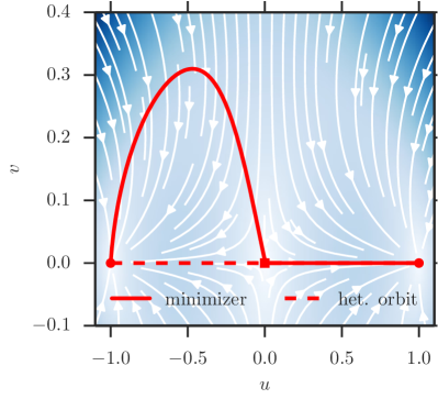
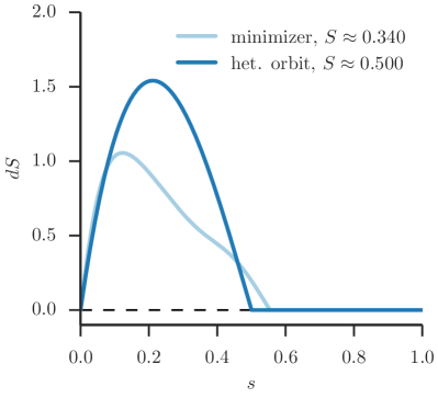
where $\beta$ is a parameter. For all values of $\beta$, the deterministic system has the two stable fixed points, $\varphi_{-}=(-1,0)$ and $\varphi_{+}=(1,0)$, and a unique unstable critical point $\varphi_{s}=(0,0)$. However it satisfies detailed balance only for $\beta=1$. In this case, we can write the drift in gradient form, $b(\varphi)=\nabla_{\varphi}U(\varphi)$, and the minimizers of the geometric action that connects $\varphi_{-}$ to $\varphi_{+}$ and vice-versa are the time-reverse of each other and lie on the location of the heteroclinic orbit where $\varphi^{\prime}\parallel\nabla U$. Here, we use $\beta=10$, in which case detailed balance is broken and the forward and backward transition pathways are no longer identical. Since the noise is additive, the system (54) falls into the category discussed in Sect. 3.4 (i.e. additive noise) and can be solved with the simplest variant of the algorithm. The minimizer of the action connecting $\varphi_{-}$ to $\varphi_{+}$ and the value of the action along it are shown in Fig. 1. Since the system is invariant under the transformation $v\to-v$, there is also a minimizer with identical action in the $v<0$ half-plane. Similarly, the paths from $\varphi_{+}$ to $\varphi_{-}$ can be obtained via the transformation $u\to-u$. The numerical parameters used in these calculations were $h=10^{-1}$, $N_{s}=2^{10}$, where $N_{s}$ denotes the number of configurations along the transition trajectory or the number of images.

Figure 1. Maier-Stein model, $\beta=10$. Left: PML and heteroclinic orbit. The arrows denote the direction of the deterministic flow, the shading its magnitude. The solid line depicts the minimizer, the dashed line the heteroclinic orbit. Dots are located at the fixed points (circle: stable; square: saddle). Right: Action density along the minimizer and the heteroclinic orbit.

4.2. Allen-Cahn/Cahn-Hilliard system

Pattern formation in motile micro-organisms is often driven by non-equilibrium forces, leading to visible patterns in cellular colonies [34, 8]. For example, E. coli in a uniform suspension separates into a bacteria-rich and a bacteria-poor phase if the swim speed decreases sufficiently rapidly with density [37]. Here we study a model inspired by these phenomena. We note that this model does not permit the thermodynamic mapping used in [37], so that understanding the non-equilibrium transitions in the model requires minimization of the geometric action of LDT.

4.2.1. Reduced Allen-Cahn/Cahn-Hilliard model

Figure 2. Allen-Cahn/Cahn-Hilliard toy ODE model, $\alpha=0.01$. The arrows denote the direction of the deterministic flow, the color its magnitude. The white dashed line corresponds to the slow manifold. The solid line depicts the minimizer, the dashed line the heteroclinic orbit. Markers are located at the fixed points (circle: stable; square: saddle).

Figure 3. Left: Action density along the path for the 2-dimensional reduced model. Path parameter is normalized to $s\in(0,1)$. For the second half of the transition, the action density is zero. Right: Minimizers of the action functional for different values of $\alpha$. For $\alpha\to 0$, the minimizer approaches the slow manifold. Note that the switch to a straight line minimizer happens at a finite value $\alpha\approx 1.12$.

Consider the SDE system

(55) $$d\phi=(\frac{1}{\alpha}Q(\phi-\phi^{3})-\phi)dt+\sqrt{\epsilon}dW$$

with $\phi=(\phi_{1},\phi_{2})$ and the matrix $Q=((1,-1),(-1,1))$. This system does not satisfy detailed balance, as its drift is made of two gradient terms with incompatible mobility operators (namely $Q$ and Id). Model (55) can be seen as a 2-dimensional reduction to a discretized version of the continuous Allen-Cahn/Cahn-Hilliard model discussed later in Sect. 4.2.2.

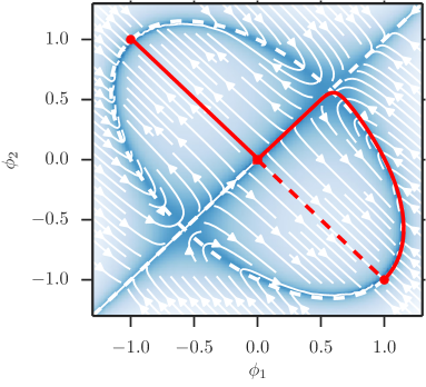
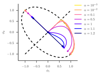
The deterministic flowlines of (55) are depicted in Fig. 2. The deterministic dynamics has two stable fixed points, $\phi_{A}=(-1,1)$ and $\phi_{B}=(1,-1)$, and an unstable critical point, $\phi_{S}=(0,0)$, lying on the separatrix where $\phi_{1}=\phi_{2}$ between the basins of $\phi_{A}$ and $\phi_{B}$. The location of the heteroclinic orbits connecting $\phi_{S}$ to $\phi_{A}$ and $\phi_{B}$ is a straight line between these points. When $\alpha$ is small in (55), there exists a “slow manifold”, comprised of all points where $Q(\phi-\phi^{3})=0$ which is shown as a white dashed line in Fig. 2 . On this manifold, the deterministic dynamics are of order $O(1)$, which is small in comparison to the dynamics of the $Q$-term, which are of order $O(1/\alpha)$. This suggests that for small enough $\alpha$ the transition trajectory will follow this slow manifold on which the drift is small, rather than the heteroclinic orbit, to escape the basin of the stable fixed points. This is confirmed in Fig. 2 where we show the action minimizer connecting $\phi_{B}$ to $\phi_{A}$. As can be seen, the minimizer first tracks the slow manifold, and it approaches the separatrix at a point far from $\phi_{S}$. It then follows closely the separatrix towards $\phi_{S}$ (which has to be part of the transition) to cross into the other basin and then relax (deterministically) towards $\phi_{A}$.

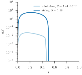
The action along the minimizer and the paths made of the heteroclinic orbits are depicted in Fig. 3 (left). Notably, due to its movement along the slow manifold, the action along the minimizer is smaller by a factor of order $\alpha$. Minimizers for different values of $\alpha$ are shown in Fig. 3 (right). Note that in the opposite limit $\alpha\gg 0$ the switch to a straight line happens at a finite value $\alpha\approx 1.12$.

In these computations, we used $N_{s}=2^{14}$, $h=10^{-2}$.

4.2.2. Full Allen-Cahn/Cahn-Hilliard model

Consider next the SPDE

(56) $$\phi_{t}=\frac{1}{\alpha}P(\kappa\phi_{xx}+\phi-\phi^{3})-\phi+\sqrt{\epsilon}\eta(x,t)\,,$$

where $P$ is an operator with zero spatial mean and $\eta(x,t)$ a spatio-temporal white-noise. This model is again of the form of two competing gradient flows with different mobilities:

(57) $$\phi_{t}=-M_{1}D_{\phi}V_{1}(\phi)-M_{2}D_{\phi}V_{2}(\phi)+\sqrt{\epsilon}M_{2}^{1/2}\eta(x,t)\,,$$

with

(58a) $$V_{1}(\phi) =\frac{1}{2}\kappa|\phi_{x}|^{2}+\frac{1}{2}|\phi|^{2}-\frac{1}{4}|\phi|^{4}, M_{1} =\frac{1}{\alpha}P$$

(58b) $$V_{2}(\phi) =-\frac{1}{2}|\phi|^{2}, M_{2} =\textrm{Id}\,.$$

For $P=-\partial_{x}^{2}$ the system is a mixture of a stochastic Allen-Cahn [2] and Cahn-Hilliard [7] equation. Here we will consider $P(\phi)=\phi-\mathchoice{{\vbox{\hbox{$\textstyle-$ }}\kern-7.83337pt}}{{\vbox{\hbox{$\scriptstyle-$ }}\kern-5.90005pt}}{{\vbox{\hbox{$\scriptscriptstyle-$ }}\kern-4.75003pt}}{{\vbox{\hbox{$\scriptscriptstyle-$ }}\kern-4.25003pt}}\!\int\phi\,dx$, which is similar in most aspects discussed below but simpler to handle numerically. We are again interested in situations where $\alpha$ is small, and the time scales associated with $V_{1}$ and $V_{2}$ differ significantly. In this case it will turn out that transition pathways are very different from the heteroclinic orbits, in that the separatrix between the basins of attraction is approached far from the unstable critical point of the deterministic system. This behavior is reminiscent of the 2-dimensional example discussed above, but in an SPDE setting.

The fixed points of the deterministic ($\epsilon=0$) dynamics of system  (56) are the solutions of

(59) $$P(\kappa\phi_{xx}+\phi-\phi^{3})-\alpha\phi=0\,.$$

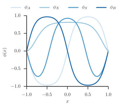
The only constant solution of this equation is the trivial fixed point $\phi(x)=0$, whose stability depends on $\alpha$ and $\kappa$. In the following, we choose $\alpha=10^{-2}$ and $\kappa={2\cdot 10^{-2}}$, in which case $\phi(x)=0$ is unstable. The two stable fixed points obtained by solving (59) for these values of $\alpha$ and $\kappa$ are depicted in Fig. 4 as $\phi_{A}$ and $\phi_{B}$, with $\phi_{A}=-\phi_{B}$. An unstable fixed point configuration on the separatrix between $\phi_{A}$ and $\phi_{B}$ is also shown as $\phi_{S}$.

Figure 4. The configurations $A,B,S,X$ in space: $\phi_{A}$ and $\phi_{B}$ are the two stable fixed points, $\phi_{S}$ is the unstable fixed point on the separatrix in between. At point $\phi_{X}$, the slow manifold intersects the separatrix.

Figure 5. Transition pathways between two stable fixed points of equation (56) in the limit $\epsilon\to 0$. Left: heteroclinic orbit, defining the deterministic relaxation dynamics from the unstable point $S$ down to either $A$ or $B$. Right: Minimizer of the geometric action, defining the most probable transition pathway from $A$ to $B$, following the slow manifold up to $X$, where it starts to nearly deterministically travel close to the separatrix into $S$.

For finite but small $\alpha$, the deterministic part of (56) has a “slow manifold” made of the solutions of

(60) $$P(\kappa\phi_{xx}+\phi-\phi^{3})=0\,.$$

On this manifold the motion is driven solely by changing the mean via the slow terms, $-\phi+\sqrt{\epsilon}\,\eta(x,t)$, on a time-scale of order $O(1)$ in $\alpha$. After two integrations in space, (60) can be written as

(61) $$\kappa\phi_{xx}+\phi-\phi^{3}=\lambda\,,$$

where $\lambda$ is a parameter. As a result the slow manifold can be described as one-parameter families of solutions parametrized by $\lambda\in\mathbb{R}$ – in general there is more than one family because the manifold can have different branches corresponding to solutions of (59) with a different number of domain walls. The configuration labeled as $\phi_{X}$ in Fig. 4 shows the field at the intersection of one of these branches with the separatrix. Since the deterministic drift along the slow manifold is small compared to the $O(1/\alpha)$ drift induced by the Cahn-Hilliard term, one expects that the most probable transition pathway will use this manifold as channel to escape the basin of attraction of the stable fixed points $\phi_{A}$ or $\phi_{B}$. This intuition is confirmed by the numerics, as shown next.

Figure 6. Projection of the heteroclinic orbit and the minimizer of the action functional into a 2-dimensional plane. The $x$-direction is proportional to its component in the direction of the initial condition $\phi_{A}$ while the $y$-direction corresponds to its spatial mean. The stable fixed points are located at $A$ and $B$, the unstable fixed point at $S$. The separatrix is the straight line $\int\phi(x)\phi_{A}(x)\,dx=0$. The heteroclinic orbit (light) travels $A\to S\to B$ in a horizontal line with vanishing mean, while the minimizer (dark) travels first along the slow manifold (dashed) $A\to X$ and then tracks the separatrix from $X$ to $S$.

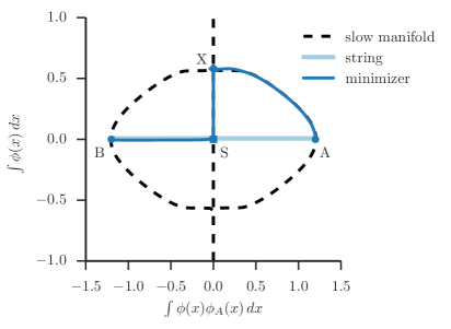
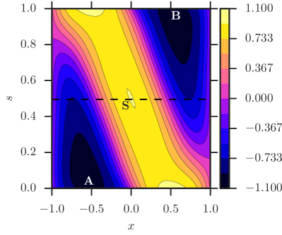
Fig. 5 (left) shows the heteroclinic orbit connecting the two stable fixed points $\phi_{A}$ and $\phi_{B}$ to the unstable configuration $\phi_{S}$. The mean is preserved along this orbit, which involves a nucleation event at the boundaries followed by domain wall motion through the domain. The unstable fixed point $\phi_{s}$, denoted by $S$, which also demarcates the position at which the separatrix is crossed, is the spatially symmetric configuration with a positive central region and two negative regions at the boundary. Locations $A$ and $B$ label the two stable fixed points $\phi_{A}$ and $\phi_{B}$.

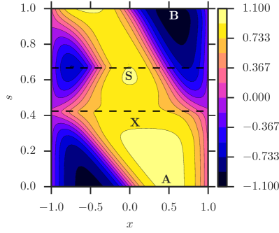
In contrast, Fig. 5 (right) shows the minimizer of the geometric action, which is the most probable transition path as $\epsilon\to 0$. It was computed via the algorithm outlined in Sect. 3.7, with $L=\frac{1}{\alpha}P\kappa\partial_{x}^{2}-\textrm{Id}$ and $R(u)=\frac{1}{\alpha}P(u-u^{3})$. Starting at the fixed point $A$ the minimizer takes a very different path than the heteroclinic orbit. It first moves the domain wall, at vanishing cost for $\alpha\to 0$, without nucleation. At the point $X$ the motion changes, tracking closely the separatrix towards the unstable point $S$. From this point onward, $S\to B$, the transition path then follows the heteroclinic orbit, which is the deterministic relaxation path. In this respect, the SPDE model (56) resembles closely the 2-dimensional model (55).

To further illustrate this resemblance, we choose to project the minimizer and the heteroclinic orbit onto two coordinates,

1. its mean $\int\phi(x)\,dx$, which resembles the direction $\phi_{1}+\phi_{2}$ of the 2-dimensional model, and

2. its component in the direction of the initial (or final) state, $\int\phi(x)\phi_{A}(x)\,dx$, which corresponds to the direction $\phi_{1}-\phi_{2}$ of the 2-dimensional model.

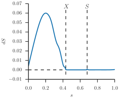
The transition path and the heteroclinic projected in these reduced coordinates are depicted in Fig. 6. Note that this figure is not a schematic, but the actual projection of the heteroclinic orbit and the minimizer of Fig. 5 according to (i) and (ii) above. The separatrix is the straight line $\int\phi(x)\phi_{A}(x)\,dx=0$. The movement of the minimizer (dark) closely along the slow manifold (dashed), $A\to X$, and the separatrix, $X\to S$, (which is also part of the slow manifold) into $S$ highlights its difference with the heteroclinic orbit (light). The configurations at the points $A,B,S$ and $X$ are depicted in Fig. 4, while Fig. 7 shows the action density $dS$ along the transition path. Note that this quantity becomes close to zero already at $X$, because the minimizer follows closely the separatrix from $X$ to $S$, and this motion is therefore quasi-deterministic.

Figure 7. Action along the minimizer. Note that the action is non-zero climbing up the slow-manifold, but diminishes to zero already at $X$ when it approaches the separatrix, before it reaches $S$.

The numerical parameters we used in these computations are $h=10^{-1}$, $N_{s}=100$, $N_{x}=2^{6}$, where $N_{x}$ denotes the number of spatial discretization points.

4.3. Burgers-Huxley model

As a second example involving an SPDE, we consider

(62) $$u_{t}+\alpha uu_{x}-\kappa u_{xx}=f(u,x,t)+\sqrt{\epsilon}\eta(x,t)\,.$$

where $\alpha>0$ and $\kappa>0$ are parameters, and we impose periodic boundary condition on $x\in[0,1]$. Without the term $f(u,x,t)$, this is the stochastic Burgers equation which arises in a variety of fields, in particular in the context of compressible gas dynamics, traffic flow, and fluid dynamics. With the reaction term $f(u,x,t)$ added this equation is referred to as the (stochastic) Burgers-Huxley equation [42] , which has been used e.g. to describe the dynamics of neurons. The addition of a reaction term makes it possible to obtain multiple stable fixed points. As a particular case, we will consider (62) with

(63) $$f(u,x,t)=-u(1-u)(1+u)$$

so that $u_{+}=1$ and $u_{-}=-1$ are the two stable fixed points of the deterministic dynamics. We are interested in the mechanism of the noise-induced transitions between these points.

Figure 8. Burgers-Huxley equation: Minimizer switching from $u_{-}=-1$ to $u_{+}=1$. Left: $u$-field. The saddle-point is marked with a dashed line. There is a noticeable kink in the dynamics switching from uphill ($s<s_{\text{saddle}}$) to downhill ($s>s_{\text{saddle}}$) dynamics. Right: Action density along the minimizer.

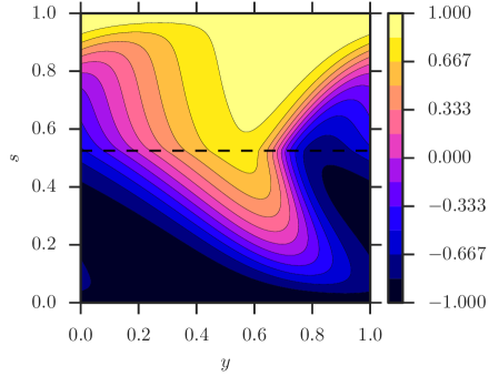
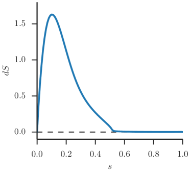
When $\alpha=0$, the system is in detailed balance and therefore the forward and backward reaction follow the same path. The potential associated with the reaction term (63) is symmetric under $u\to-u$, and both states are equally probable. In contrast, when $\alpha\neq 0$ it is not obvious a priori whether $u_{+}$ and $u_{-}$ are equally probable, since the non-linearity breaks the spatial symmetry, leading to a steepening of negative gradients into shocks while flattening positive gradients. A computation of the minimizer of the geometric action in both directions, for $\kappa=0.01$ and $\alpha=\tfrac{1}{4}$ reveals that indeed forward and backward reactions are equally probable, even though the transition paths do not coincide with the heteroclinic orbits. The transition from $u_{-}$ to $u_{+}$ is depicted in Fig. 8 (left). An intuitive explanation for the equal probability of $u_{+}$ and $u_{-}$ is given by the fact that the backward reaction pathways is identical to the forward path under the transformation $u\to-u$, $x\to-x$. The action along this minimizer is depicted in figure 8 (right). The minimizer is computed via the algorithm lined out in Sect. 3.7, with $L=-\kappa\partial_{x}^{2}$ and $R(u)=\alpha uu_{x}+u(1-u)(1+u)$.

The numerical parameters were chosen as $N_{s}=100$, $N_{x}=2^{8}$, $h=5\cdot 10^{-3}$.

4.4. Noise-induced transitions between climate regimes

Many climate systems exhibit metastability. Examples include the Kuroshio oceanic current off the coast of Japan, which can be in either a small or a large meander state and rarely switches between the two [9, 33], or the atmospheric mid-latitude circulation over the North-Atlantic, which makes rare transitions between a strongly zonal and a weakly zonal (“blocked”) flow, characterized as “Grosswetterlagen” in [4]. In these and similar examples, the climate system stays trapped in the vicinity of the stable regimes most of the time. Random noise, originating either from physical stresses or from unresolved modes in truncated models, induces rare regime transitions, which can be captured by large deviation minimizers. The transition trajectory and their corresponding action allow to make statements about not only the relative probability of the different regimes and the transition rates, but also the exact transition pathway taken to switch between regimes.

We want to illustrate the feasibility of our numerical scheme for this particular field of application by investigating metastability in two simple climate models: A three-dimensional model for Grosswetterlagen proposed by Egger [18] and the six-dimensional Charney-DeVore model [10]. Due to their highly truncated nature, both models have very limited predictive power, but exemplify the phenomenon of metastability in climate patterns or regimes.

4.4.1. Metastable climate regimes in Egger’s model

Figure 9. Egger’s model with $H=12,\beta=1.25,\gamma=2,k=2,U_{0}=10.5$ Left: Minimizers and deterministic relaxation paths. Right: Comparison of the action density.

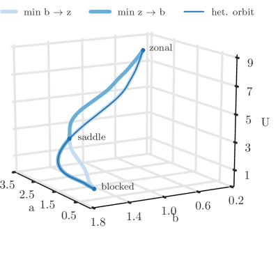
Egger [18] introduces the following SDE system as a crude model to describe weather regimes in central Europe:

(64) $$\begin{cases}da=kb(U-\beta/k^{2})\,dt-\gamma a\,dt+\sqrt{\epsilon}dW_{a}\,,\\ db=-ka(U-\beta/k^{2})\,dt+UH/k\,dt-\gamma b\,dt+\sqrt{\epsilon}dW_{b}\,,\\ dU=-bHk/2\,dt-\gamma(U-U_{0})\,dt+\sqrt{\epsilon}dW_{U}\,.\end{cases}$$

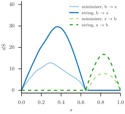
When $\epsilon$ is small, these equation exhibit metastability between a “blocked state” and a “zonal state”, shown in Fig. 9. We use our gMAM algorithm to compute the transition paths between these states. The system (64) falls into the category discussed in Sect. 3.4 (i.e. additive noise) and can be solved with the simplest variant of the algorithm. For $H=12,\beta=1.25,\gamma=2,k=2$ and $U_{0}=10.5$, the fixed points are approximately $(a,b,U)=(0.465,1.65,0.593)$ for the blocked, $(3.07,0.392,8.15)$ for the zonal and $(2.80,1.35,2.38)$ for the unstable fixed point (saddle). The minimizers of the action are show in Fig. 9(left) where they are compared to the heteroclinic orbits that connects the unstable critical points to the stable ones. The action density along the transition trajectories and the heteroclinic orbits is depicted in Fig. 9 (right).

The numerical parameters we used in these computations are $N_{s}=2^{8}$, $h=10^{-3}$.

4.4.2. Metastable climate regimes in the Charney-DeVore model

Figure 10. Contours of the stream-function $\psi(x,y)$ of the two meta-stable configurations of the 6-dimensional CDV model. Left: Zonal state; Right: Blocked state.

Figure 11. Contours of the stream-function $\psi(x,y)$ along the transition trajectory from the zonal to the blocked meta-stable configuration for the CDV model. The arclength parameter increases in lexicographic order, with the top left plot being the initial state and the bottom right plot being the final state. The saddle point configuration is depicted in the center. The colormap is identical to figure 10.

Figure 12. Contours of the stream-function $\psi(x,y)$ along the transition trajectory from the blocked to the zonal meta-stable configuration for the CDV model. The arclength parameter increases in lexicographic order, with the top left plot being the initial state and the bottom right plot being the final state. The saddle point configuration is depicted in the center. The colormap is identical to figure 10.

Figure 13. Action density $dS$ along the transition pathways from zonal to blocked (forward) and from blocked to zonal (backward). In both directions, after passing the saddle point, the action becomes zero since the motion is deterministic.

Egger’s model retains no nonlinear interaction between different fluid modes, which is believed to be insufficient to explain the transitions between zonal and blocked states. A more sophisticated model, truncating the barotropic vorticity equation (BVE) with full nonlinear terms, was introduced by Charney and DeVore [10]. Their starting point is the two-dimensional BVE on the $\beta$-plane,

(65) $$\frac{\partial}{\partial t}\omega=u\cdot\nabla\omega-C(\omega-\omega^{*})\,.$$

Here $\omega=\zeta+\beta y+\gamma h$ is the total vorticity, where $\gamma h$ is the topography in the $\beta$-plane, with $\beta=2\Omega\cos(\theta)/R$ for planetary angular velocity $\Omega$, radius $R$ and latitude $\theta$, and $\zeta=\Delta\psi$ is the relative vorticity for the stream-function $\psi$. The term $-C(\omega-\omega^{*})$ accounts for Ekman damping with coefficient $C>0$.

Charney-DeVore considered the vorticity equation (65) in the box $[0,2\pi]\times[0,\pi b]$ with periodic boundary conditions in $x$-direction and no-slip boundary conditions in $y$-direction. They then projected this equation over 6 Fourier modes in total, using the following representation for the stream-function $\psi(x,y,t)$:

(66) $$\psi(x,y,t)=\sum_{n,m}\psi_{nm}(t)\phi_{nm}(x,y)\,,$$

where the sums run on $n\in\{-1,0,1\}$ and $m\in\{1,2\}$ and

(67) $$\phi_{0m}(y) =\sqrt{2}\cos(my/b), \phi_{nm}(x,y) =\sqrt{2}e^{inx}\sin(my/b)\,.$$

Letting $x_{i}$, $i\in\{1,\dots,6\}$ be defined as

(68) $$\begin{split}x_{1}=\frac{1}{b}\psi_{01},\qquad x_{2}=\frac{1}{\sqrt{2}b}\left(\psi_{11}+\psi_{-11}\right),\qquad x_{3}=\frac{i}{\sqrt{2}b}\left(\psi_{11}-\psi_{-11}\right),\\ x_{4}=\frac{1}{b}\psi_{02},\qquad x_{5}=\frac{1}{\sqrt{2}b}\left(\psi_{12}+\psi_{-12}\right),\qquad x_{6}=\frac{i}{\sqrt{2}b}\left(\psi_{12}-\psi_{-12}\right)\,,\end{split}$$

taking the following form for the topography

(69) $$h(x,y)=\cos(x)\sin(y/b)\,,$$

and choosing $\omega^{*}$ such that only two parameters $x_{1}^{*}$ and $x_{4}^{*}$ are free and the other are set zero, they arrived at the following six-dimensional model

(70) $$\begin{split}dx_{1}&=\left(\tilde{\gamma}_{1}x_{3}-C(x_{1}-x_{1}^{*})\right)dt+\sqrt{2\epsilon}dW_{1}\,,\\ dx_{2}&=\left(-(\alpha_{1}x_{1}-\beta_{1})x_{3}-Cx_{2}-\delta_{1}x_{4}x_{6}\right)dt+\sqrt{2\epsilon}dW_{2}\,,\\ dx_{3}&=\left((\alpha_{1}x_{1}-\beta_{1})x_{2}-\gamma_{1}x_{1}-Cx_{3}+\delta_{1}x_{4}x_{5}\right)dt+\sqrt{2\epsilon}dW_{3}\,,\\ dx_{4}&=\left(\tilde{\gamma}_{2}x_{6}-C(x_{4}-x_{4}^{*})+\eta(x_{2}x_{6}-x_{3}x_{5})\right)dt+\sqrt{2\epsilon}dW_{4}\,,\\ dx_{5}&=\left(-(\alpha_{2}x_{1}-\beta_{2})x_{6}-Cx_{5}-\delta_{2}x_{3}x_{4}\right)dt+\sqrt{2\epsilon}dW_{5}\,,\\ dx_{6}&=\left((\alpha_{2}x_{1}-\beta_{2})x_{5}-\gamma_{2}x_{4}-Cx_{6}+\delta_{2}x_{2}x_{4}\right)dt+\sqrt{2\epsilon}dW_{6}\,,\end{split}$$

where, for $m\in\{1,2\}$,

(71) $$\begin{split}\alpha_{m}&=\frac{8\sqrt{2}}{\pi}\frac{m^{2}}{4m^{2}-1}\frac{b^{2}+m^{2}-1}{b^{2}+m^{2}}\,,\\ \beta_{m}&=\frac{\beta b^{2}}{b^{2}+m^{2}}\,,\\ \gamma_{m}&=\gamma\frac{\sqrt{2}b}{\pi}\frac{4m^{3}}{(4m^{2}-1)(b^{2}+m^{2})}\,,\\ \tilde{\gamma}_{m}&=\gamma\frac{\sqrt{2}b}{\pi}\frac{4m}{4m^{2}-1}\,,\\ \delta_{m}&=\frac{64\sqrt{2}}{15\pi}\frac{b^{2}-m^{2}+1}{b^{2}+m^{2}}\,,\\ \eta&=\frac{16\sqrt{2}}{5\pi}\,.\end{split}$$

The original Charney-DeVore equation did not contain random forcing terms: here we added to each equations an independent white noise $dW_{i}$ with amplitude $\sqrt{2\epsilon}$.

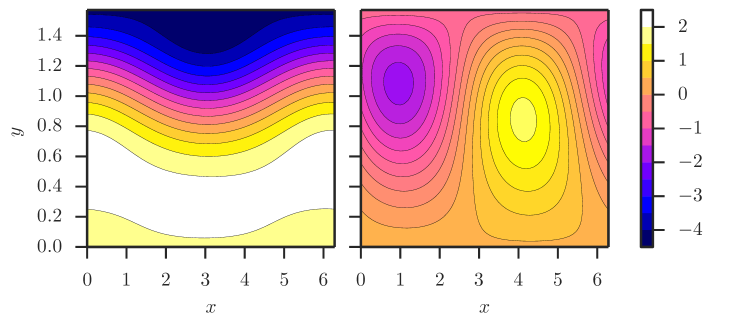
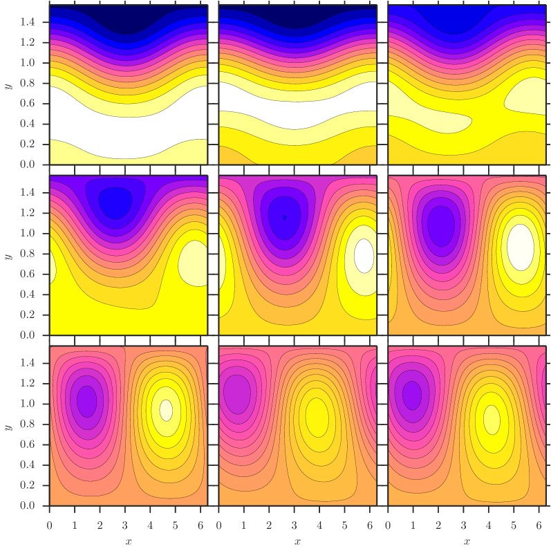
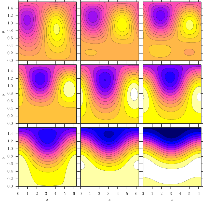
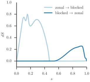
Choosing $b=\tfrac{1}{2}$, $C=\tfrac{1}{10}$, $\beta=\tfrac{5}{4}$, $\gamma=1$, $x_{1}^{*}=\tfrac{9}{2}$, and $x_{4}^{*}=-\tfrac{9}{5}$, the 6-dimensional stochastic model above possesses two metastable states, shown in Fig. 10: a zonal state (left) and a blocked state (right). The transition paths from zonal to blocked and from blocked to zonal are different. They are shown in Fig. 11 and Fig. 12, respectively, and they were both calculated by minimizing the geometric action using our simplified gMAM algorithm. The actions along both paths are depicted in Fig. 13.

The numerical parameters in these computations were $N_{s}=100$, $h=10^{-3}$.

4.5. Generalized voter/Ising model

Figure 14. Generalized voter/Ising model. Left: The arrows denote the direction of the deterministic flow, the shading its magnitude. The solid line depicts the minimizer, the dashed line the heteroclinic orbit. Markers are located at the fixed points (circle: stable; square: saddle). Right: Action density along the minimizers for the two trajectories, with normalized path parameter $s\in(0,1)$.

To analyze phase transitions in out-of-equilibrium systems, a Langevin equation was proposed in [1] that models critical phenomena with two absorbing states. This equation was constructed by requiring that it be symmetric under the transformation $\phi\to-\phi$ and have two absorbing states, arbitrarily chosen to be at $\pm 1$. The presence of these absorbing states makes the noise multiplicative, with a scaling involving the square root of the distance to the absorbing boundaries, as suggested by the voter model [13, 15]. In order to account for Ising-like spontaneous symmetry breaking, the authors of [1] also added a bi-stable “potential”-term with $-V^{\prime}(\phi)=(a\phi-b\phi^{3})$ to the equation, which finally lead them to:

(72) $$\phi_{t}=\left((1-\phi^{2})(a\phi-b\phi^{3})+D\phi_{xx}\right)\,dt+\sigma\sqrt{1-\phi^{2}}\eta(x,t)\,.$$

In the absence of noise ($\epsilon=0$) and for $a>0$, the $\phi=0$ state is locally unstable, but $b>0$ ensures stable fixed points at $\phi=\pm\sqrt{a/b}$. In the limit $a/b\to 1$, these fixed points approach the absorbing boundaries, and we are interested in the noise induced transition between these states.

We stress that making mathematical sense of (72) is non-trivial (see the discussion in Sect. 3.7). In the present application, we are going to consider a finite truncation of this SPDE, where the question of spatial regularity disappears. Specifically, we transform (72) into a two-dimensional stochastic ODE model by discretizing the spatial direction via the standard 3-point Laplace stencil, and taking only $N_{x}=2$ discretization points. This yields the stochastic ODE system

(73) $$\begin{cases}d\phi_{1}&=\left((1-\phi_{1}^{2})(a\phi_{1}-b\phi_{1}^{3})+D(\phi_{1}-\phi_{2})\right)\,dt+\sigma\sqrt{1-\phi_{1}^{2}}\,dW_{x}\\ d\phi_{2}&=\left((1-\phi_{2}^{2})(a\phi_{2}-b\phi_{2}^{3})-D(\phi_{1}-\phi_{2})\right)\,dt+\sigma\sqrt{1-\phi_{2}^{2}}\,dW_{y}\,,\end{cases}$$

where the constant $D$ couples the two degrees of freedom. This SDE poses an interesting test-case for our numerical scheme, since not only the noise is multiplicative, but also the computational domain must be restricted. The square defined by $1=\max(|\phi_{1}|,|\phi_{2}|)$ marks the region in which the noise is defined (real), and the noise decreases towards zero as it approaches this absorbing barrier. Analog to the discussion in [1], the choice of the parameters $(a,b)$ determines the dynamics, in particular if $a>0,b>0$ the model exhibits bi-stability: There is an unstable fixed point at $\phi=(0,0)$ and stable fixed points at $\phi=\pm(\sqrt{a/b},\sqrt{a/b})$. As long as $a<b$, these fixed points are inside the allowed region. For $a/b\to 1$ the two stable fixed points approach the absorbing boundary. Here, we take $b=1,a=1-10^{-4},D=0.4$, so that $\sqrt{a/b}\approx 0.99995$ is located close to the barrier at $1$. The minimizer and corresponding action are shown in Fig. 14.

The numerical parameters were chosen as $N_{s}=2^{8}$, $h=10^{-3}$.

4.6. Bi-stable reaction-diffusion model

In the context of chemical reactions and birth-death processes, one considers networks of several reactants in a container of volume $V$ which is considered well-stirred. As an example case, we consider the bi-stable chemical reaction network

$$A\underset{k_{1}}{\stackrel{{\scriptstyle k_{0}}}{{\rightleftharpoons}}}X,\qquad 2X+B\underset{k_{3}}{\stackrel{{\scriptstyle k_{2}}}{{\rightleftharpoons}}}3X$$

with rates $k_{i}>0$, and where the concentrations of $A$ and $B$ are held constant. This system was introduced in [32] as a prototypical model for a bi-stable reaction network. Its dynamics can be modeled as a Markov jump process (MJP) with generator

(74) $$(L^{R}f)(n)=A_{+}(n)\left(f(n+1)-f(n)\right)+A_{-}(n)\left(f(n-1)-f(n)\right)$$

with the propensity functions

(75) $$\begin{cases}A_{+}(n)&=k_{0}V+(k_{2}/V)n(n-1)\\ A_{-}(n)&=k_{1}n+(k_{3}/V^{2})n(n-1)(n-2)\,.\end{cases}$$

The model above satisfies a large deviation principle in the following scaling limit: Denote by $c=n/V$ the concentration of $X$, and normalize it by a typical concentration, $\rho=c/c_{0}$. Now, in the limit of a large number of particles per cell $\Omega=c_{0}V$ and simultaneously rescaling time by $1/\Omega$, we obtain

(76) $$(L_{\epsilon}^{R}f)(\rho)=\frac{1}{\epsilon}\Big{(}a_{+}(\rho)\left(f(\rho+\epsilon)-f(\rho)\right)+a_{-}(\rho)\left(f(\rho-\epsilon)-f(\rho)\right)\Big{)}\,,$$

where $\epsilon=1/\Omega$ is a small parameter. Here, we defined $k_{i}=\lambda_{i}(c_{0})^{1-i}$, and

(77) $$\begin{cases}a_{+}(\rho)&=\lambda_{0}+\lambda_{2}\rho^{2}\\ a_{-}(\rho)&=\lambda_{1}\rho+\lambda_{3}\rho^{3}\,.\end{cases}$$

The large deviation principle for (76) can be formally obtained via WKB analysis, that is, by setting $f(\rho)=e^{\epsilon^{-1}G(\rho)}$ in (76) and expanding in $\epsilon$ [14]. To leading order in $\epsilon$, this gives an Hamilton-Jacobi operator associated with an Hamiltonian that is also the one rigorously derived in LDT [35]. It reads

(78) $$H(\rho,\vartheta)=a_{+}(\rho)(e^{\vartheta}-1)+a_{-}(\rho)(e^{-\vartheta}-1)\,.$$

This is an example of a system whose Hamiltonian is not quadratic in the conjugate momentum $\vartheta$. Therefore the computation of $\vartheta_{*}$ by (26) can not be performed explicitly in general. For parameters $\lambda_{0}=0.8,\lambda_{1}=2.9,\lambda_{2}=3.1,\lambda_{3}=1$, the system has two stable fixed points $\rho_{\pm}$ and a saddle $\rho_{s}$ at $\rho_{+}=\tfrac{8}{5},\rho_{-}=\tfrac{1}{2},\rho_{s}=1$.

Since transitions in 1D are fairly trivial, we want to consider the case of $N$ neighboring reaction compartments, each well-stirred, but with random jumps possible between neighboring compartments. This situation was analyzed in [38] via direct sampling, but we are interested in the computation of the transition trajectory. Denote by $\rho_{i}$ the concentration in the $i$-th compartment and refer to the vector ${\rho}$ as the complete state, ${\rho}=\sum_{i=0}^{N}\rho_{i}\hat{e}_{i}$. In this case, we obtain a diffusive part of the generator, $L^{D}$, coupling neighboring compartments. For a diffusivity $D$, it is

(79) $$(L^{D}f)({\rho})=\frac{D}{\epsilon}\sum_{i=1}^{N}\rho_{i}\left(f({\rho}-\epsilon\hat{e}_{i}+\epsilon\hat{e}_{i-1})+f({\rho}-\epsilon\hat{e}_{i}+\epsilon\hat{e}_{i+1})-2f({\rho})\right)\,.$$

The process associated with this generator also admits a large deviation principle with Hamiltonian

(80) $$H^{D}({\rho},{\vartheta})=D\sum_{i=1}^{N}\rho_{i}\left(e^{\vartheta_{i-1}-\vartheta_{i}}+e^{\vartheta_{i+1}-\vartheta_{i}}-2\right)\,.$$

Therefore, the full Hamiltonian becomes $H({\rho},{\vartheta})=H^{D}({\rho},{\vartheta})+\sum_{i=1}^{N}H^{R}(\rho_{i},\vartheta_{i})$, where $H^{R}(\rho_{i},\vartheta_{i})$ is the reactive Hamiltonian in (78), which is summed up over all the compartments.

Figure 15. Bi-Stable reaction-diffusion model with $N=2$ reaction cells. Show are the forward (red) and backward (green) transitions between the two stable fixed points, in comparison to the heteroclinic orbit (dashed). The flow-lines depict the deterministic dynamics, their magnitude is indicated by the background shading.

Figure 16. Action densities for the bi-stable reaction-diffusion model. Depicted are the actions corresponding to the forward (solid) and backward (dashed) minimizer (dark) and heteroclinic (light) orbit.

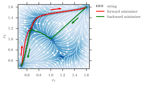
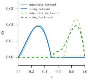
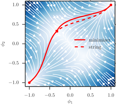
We used our new gMAM algorithm to minimize the geometric action and compute the transition paths between the stable fixed points for the simplest non-trivial case of $N=2$ compartments. Shown in Fig. 15 are the forward and backward trajectories. Note that the backward transition ($(\rho_{+},\rho_{+})\to(\rho_{-},\rho_{-})$) takes a special form: It climbs against the deterministic dynamics up to the maximum, then relaxes along the separatrix down to the saddle. Additionally, we compare these trajectories with the heteroclinic orbit obtained by the string method. The action along these trajectories is depicted in Fig. 16. Note how for the backward minimizer the action is zero already before it hits the saddle, as the movement from the maximum to the saddle happens deterministically.

The numerical parameters were chosen as $N_{s}=2^{9}$, $h=10$.

4.7. Slow-fast systems

In contrast to a large deviation principle arising in the limit of small noise or large number of particles, a different class of Hamiltonians arises for systems with a slow variable $X$ evolving on a timescale $O(1)$ and a fast variable $Y$ on a time scale $O(\alpha)$:

(81a) $$\dot{X} =f(X,Y)$$

(81b) $$dY =\frac{1}{\alpha}b(X,Y)dt+\frac{1}{\sqrt{\alpha}}\sigma(X,Y)dW\,.$$

Examples of systems with large timescale separation $\alpha\ll 1$ are ubiquitous in nature, and usually one is interested mostly in the long-time behavior of the slow variables. In particular, we are concerned with situations where the slow dynamics exhibits metastability. We want to use our algorithm to compute transition pathways in this setup for the limit of infinite time scale separation.

In the limit as $\alpha\to 0$, the fast variables reach statistical equilibrium before any motion of the slow variables, and these slow variables only experience the average effect of the slow ones. This behavior can be captured by the following deterministic limiting equation which is akin to a law of large numbers (LLN) in the present context and reads

(82) $$\dot{\bar{X}}=F(\bar{X})\quad\text{where}\quad F(x)=\lim_{T\to\infty}\frac{1}{T}\int_{0}^{T}f(x,Y_{x}(\tau))\,d\tau\,.$$

Here $Y_{x}(t)$ is the solution of (81b) for $X(t)=x$ fixed [19, 3, 30, 6]. For small but finite $\alpha$, the slow variables also experience fluctuations through the fast variables. In particular, the statistics of $\xi=(X-\bar{X})/\sqrt{\alpha}$ on $O(1)$ time scales can be described by a central limit theorem (CLT) as small Gaussian noise on top of the slow mean $\bar{X}$. The CLT scaling, however, is inappropriate to describe the fluctuations of the slow variables that are induced by the effect of the fast variables on longer time scales and may, for example, lead to transitions between stable fixed points of the limiting equation in (82). In particular, the naive procedure of constructing an SDE out of the LLN and CLT to then compute its LDT fails. Instead, the transitions in the limit of $\alpha\to 0$ are captured by an LDP with the Hamiltonian

(83) $$H(x,\vartheta)=\lim_{T\to\infty}\frac{1}{T}\log\mathbb{E}\exp\left(\vartheta\int_{0}^{T}f(x,Y_{x}(t))\,dt\right)\,.$$

Except for the special case $f(x,y)=r(x)+s(y)y$ (linear dependence on the fast variable), the Hamiltonian (83) is non-quadratic in $\theta$. As a consequence no S(P)DE with Gaussian noise exists for the slow variable which has an LDP to describe the transitions correctly.

The implicit nature of the Hamiltonian (83), in particular containing an expectation, complicates numerical procedures to compute its associated minimizers. Yet, in the non-trivial case of a quadratic dependence of the slow variable on the fast ones, for example,

(84) $$\begin{cases}\dot{X}=Y^{2}-\beta X\\ \displaystyle dY=-\frac{1}{\alpha}\gamma(X)Y\,dt+\frac{\sigma}{\sqrt{\alpha}}dW\,,\end{cases}$$

one indeed does obtain an explicit formula for the Hamiltonian (83) (as derived in [6])

(85) $$h(x,\vartheta)=-\beta x\vartheta+\tfrac{1}{2}\left(\gamma(x)-\sqrt{\gamma^{2}(x)-2\sigma^{2}\vartheta}\right)\,.$$

This example is interesting for our purpose not only because the Hamiltonian is non-quadratic, but furthermore because of the existence of a forbidden region $\vartheta>\gamma^{2}/(2\sigma)$ where the Hamiltonian is not defined.

Figure 17. Coupled slow-fast system ODE model for $D=1.0$. Left: The arrows denote the direction of the deterministic flow, the shading its magnitude. The solid line depicts the minimizer, the dashed line the relaxation paths from the saddle. Markers are located at the fixed points (circle: stable; square: saddle). Right: Action density along the minimizers for the two trajectories up to the saddle, with normalized path parameter $s\in(0,1)$.

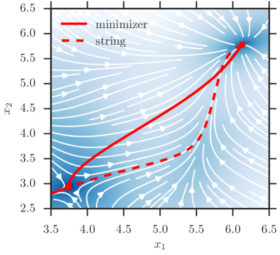
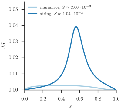
Additionally increasing the number of degrees of freedom by combining two independent multi-stable slow-fast systems and coupling them by a spring with spring constant $D$, the full system reads

(86) $$\begin{cases}\dot{X}_{1}=Y_{1}^{2}-\beta_{1}X_{1}-D(X_{1}-X_{2})\\ \dot{X}_{2}=Y_{2}^{2}-\beta_{2}X_{2}-D(X_{2}-X_{1})\\ \displaystyle dY_{1}=-\frac{1}{\alpha}\gamma(X_{1})Y_{1}dt+\frac{\sigma}{\sqrt{\alpha}}dW_{1}\\ \displaystyle dY_{2}=-\frac{1}{\alpha}\gamma(X_{2})Y_{2}dt+\frac{\sigma}{\sqrt{\alpha}}dW_{2}\,.\end{cases}$$

The Hamiltonian for the LDT for this system is

(87) $$H(x_{1},x_{2},\vartheta_{1},\vartheta_{2})=h(x_{1},\vartheta_{1})+h(x_{2},\vartheta_{2})+\langle-\nabla U(x_{1},x_{2}),\vartheta\rangle\,,$$

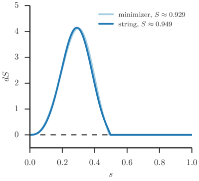
for $U(x,y)=\frac{1}{2}D(x-y)^{2}$ and $h(x,\vartheta)$ defined as in equation (85). The choice $\gamma(X)=(X-5)^{2}+1$ ensures two stable fixed points. The deterministic dynamics of this system (i.e. the evolution of the averaged slow variables) are depicted as white arrows in Fig. 17 (left). To stress the important portion of the transition trajectory, the plot is focused only on the initial state up to the saddle. Compared are the minimizer and the heteroclinic orbits connecting the stable fixed points to the saddle point. The corresponding actions are shown in Fig. 17 (right). The specific choice of model parameters for this computation is $\beta_{1}=0.6,\beta_{2}=0.3,D=1.0$ and $\sigma^{2}=10$.

The numerical parameters were chosen as $N_{s}=2^{10}$, $h=10^{-2}$.

5. Concluding Remarks

We have discussed numerical schemes to compute minimizers of large deviation action functionals, which are based on the geometric minimum action method. The basis of these schemes is the minimization of a geometric action on the space of arc-length parametrized curves, which makes it possible to perform the double minimization over transition time $T$ and action $S_{T}$ that is required to compute the LDT quasipotential. In particular, transitions between metastable fixed points of a system, which generally involve $T\to\infty$ and which are not tractable with non-geometric minimum action methods can be naturally analyzed in this setup.

A simplified gMAM algorithm was proposed here which is based on a particular formulation of the geometric action leading to a mixed optimization problem. This new formulation of the gMAM algorithm is easier to implement than the original method: In its simplest form, only first order derivatives of the Hamiltonian $H(\varphi,\vartheta)$ are needed. The algorithm is applicable to a large class of systems, and does not rely on an explicit formula of the large deviation rate function – only the Hamiltonian of the theory is needed. We derived specific reductions that are possible in regularly occurring special cases, such as SDEs with additive or multiplicative noise. Furthermore, we discussed optimizations for SPDEs with additive noise and commented on how to improve numerical efficiency.

The performances of the new gMAM algorithm were illustrated in a series of applications arising from different fields and involving different types of models, like S(P)DEs with additive and multiplicative Gaussian noises, Markov jump processes, or slow-fast systems.

Acknowledgement

We would like to thank M. Cates, A. Donev, and F. Bouchet for helpful discussions. This research was supported in part by the NSF grants DMR-1207432 (T. Grafke), DMS-1108780 and DMS-1522737 (T. Schäfer), and DMS-1522767 (E. Vanden-Eijnden).

References

- Al Hammal et al. [2005] Omar Al Hammal, Hugues Chaté, Ivan Dornic, and Miguel A. Muñoz. Langevin Description of Critical Phenomena with Two Symmetric Absorbing States. Physical Review Letters, 94(23):230601, June 2005. doi:10.1103/PhysRevLett.94.230601.
- Allen and Cahn [1972] S.M Allen and J.W Cahn. Ground state structures in ordered binary alloys with second neighbor interactions. Acta Metallurgica, 20(3):423–433, March 1972. ISSN 00016160. doi:10.1016/0001-6160(72)90037-5.
- Bakhtin [2003] Victor I. Bakhtin. Cramér’s asymptotics in systems with fast and slow motions. Stochastics and Stochastic Reports, 75(5):319–341, October 2003. ISSN 1045-1129. doi:10.1080/1045112031000155669.
- Baur [1951] Franz Baur. Extended range weather forecasting. Compendium of meteorology, pages 814–833, 1951.
- Beylkin et al. [1998] Gregory Beylkin, James M. Keiser, and Lev Vozovoi. A New Class of Time Discretization Schemes for the Solution of Nonlinear PDEs. Journal of Computational Physics, 147(2):362–387, December 1998. ISSN 00219991. doi:10.1006/jcph.1998.6093.
- Bouchet et al. [2016] Freddy Bouchet, Tobias Grafke, Tomàs Tangarife, and Eric Vanden-Eijnden. Large Deviations in Fast-Slow Systems. Journal of Statistical Physics, pages 1–20, January 2016. ISSN 0022-4715, 1572-9613. doi:10.1007/s10955-016-1449-4.
- Cahn and Hilliard [1958] John W. Cahn and John E. Hilliard. Free Energy of a Nonuniform System. I. Interfacial Free Energy. The Journal of Chemical Physics, 28(2):258–267, February 1958. ISSN 0021-9606, 1089-7690. doi:10.1063/1.1744102.
- Cates et al. [2010] M. E. Cates, D. Marenduzzo, I. Pagonabarraga, and J. Tailleur. Arrested phase separation in reproducing bacteria creates a generic route to pattern formation. Proceedings of the National Academy of Sciences, 107(26):11715–11720, June 2010. ISSN 0027-8424, 1091-6490. doi:10.1073/pnas.1001994107.
- Chao [1984] Shenn-Yu Chao. Bimodality of the Kuroshio. Journal of Physical Oceanography, 14(1):92–103, January 1984. ISSN 0022-3670. doi:10.1175/1520-0485(1984)014<0092:BOTK>2.0.CO;2.
- Charney and DeVore [1979] Jule G. Charney and John G. DeVore. Multiple Flow Equilibria in the Atmosphere and Blocking. Journal of the Atmospheric Sciences, 36(7):1205–1216, July 1979. ISSN 0022-4928. doi:10.1175/1520-0469(1979)036<1205:MFEITA>2.0.CO;2.
- Chernykh and Stepanov [2001] A. I. Chernykh and M. G. Stepanov. Large negative velocity gradients in Burgers turbulence. Physical Review E, 64(2):026306, July 2001. doi:10.1103/PhysRevE.64.026306.
- Cox and Matthews [2002] S.M. Cox and P.C. Matthews. Exponential Time Differencing for Stiff Systems. Journal of Computational Physics, 176(2):430–455, March 2002. ISSN 00219991. doi:10.1006/jcph.2002.6995.
- Dickman and Tretyakov [1995] Ronald Dickman and Alex Yu. Tretyakov. Hyperscaling in the Domany-Kinzel cellular automaton. Physical Review E, 52(3):3218–3220, September 1995. doi:10.1103/PhysRevE.52.3218.
- Doering et al. [2007] Charles R Doering, Khachik V Sargsyan, Leonard M Sander, and Eric Vanden-Eijnden. Asymptotics of rare events in birth-death processes bypassing the exact solutions. Journal of Physics: Condensed Matter, 19(6):065145, February 2007. ISSN 0953-8984, 1361-648X. doi:10.1088/0953-8984/19/6/065145.
- Dornic et al. [2001] Ivan Dornic, Hugues Chaté, Jérôme Chave, and Haye Hinrichsen. Critical Coarsening without Surface Tension: The Universality Class of the Voter Model. Physical Review Letters, 87(4):045701, July 2001. doi:10.1103/PhysRevLett.87.045701.
- E et al. [2002] Weinan E, Weiqing Ren, and Eric Vanden-Eijnden. String method for the study of rare events. Physical Review B, 66(5):052301, August 2002. doi:10.1103/PhysRevB.66.052301.
- E et al. [2004] Weinan E, Weiqing Ren, and Eric Vanden-Eijnden. Minimum action method for the study of rare events. Communications on Pure and Applied Mathematics, 57(5):637–656, May 2004. ISSN 1097-0312. doi:10.1002/cpa.20005.
- Egger [1981] J. Egger. Stochastically Driven Large-scale Circulations with Multiple Equilibria. Journal of the Atmospheric Sciences, 38(12):2606–2618, December 1981. ISSN 0022-4928. doi:10.1175/1520-0469(1981)038<2606:SDLSCW>2.0.CO;2.
- Freidlin [1978] M. I. Freidlin. The Averaging Principle and Theorems on Large Deviations. Russian Mathematical Surveys, 33:117–176, October 1978. doi:10.1070/RM1978v033n05ABEH002516.
- Freidlin and Wentzell [2012] Mark I Freidlin and Alexander D Wentzell. Random perturbations of dynamical systems, volume 260. Springer, 2012.
- Grafke et al. [2014] Tobias Grafke, Rainer Grauer, Tobias Schäfer, and E. Vanden-Eijnden. Arclength Parametrized Hamilton’s Equations for the Calculation of Instantons. Multiscale Modeling & Simulation, 12(2):566–580, January 2014. ISSN 1540-3459. doi:10.1137/130939158.
- Grafke et al. [2015] Tobias Grafke, Rainer Grauer, and Stephan Schindel. Efficient Computation of Instantons for Multi-Dimensional Turbulent Flows with Large Scale Forcing. Communications in Computational Physics, 18(03):577–592, September 2015. ISSN 1991-7120. doi:10.4208/cicp.031214.200415a.
- Hairer [2014] M. Hairer. A theory of regularity structures. Inventiones mathematicae, 198(2):269–504, March 2014. ISSN 0020-9910, 1432-1297. doi:10.1007/s00222-014-0505-4.
- Hairer and Weber [2015] Martin Hairer and Hendrik Weber. Large deviations for white-noise driven, nonlinear stochastic PDEs in two and three dimensions. Annales de la faculté des sciences de Toulouse Mathématiques, 24(1):55–92, 2015. ISSN 0240-2963. doi:10.5802/afst.1442.
- Heymann and Vanden-Eijnden [2008a] M. Heymann and E. Vanden-Eijnden. Pathways of maximum likelihood for rare events in nonequilibrium systems: application to nucleation in the presence of shear. Phys. Rev. Lett., 100(14):140601, 2008a.
- Heymann and Vanden-Eijnden [2008b] Matthias Heymann and Eric Vanden-Eijnden. The geometric minimum action method: A least action principle on the space of curves. Communications on Pure and Applied Mathematics, 61(8):1052–1117, August 2008b. ISSN 1097-0312. doi:10.1002/cpa.20238.
- Kassam and Trefethen [2005] A. Kassam and L. Trefethen. Fourth-Order Time-Stepping for Stiff PDEs. SIAM Journal on Scientific Computing, 26(4):1214–1233, January 2005. ISSN 1064-8275. doi:10.1137/S1064827502410633.
- Kifer [1992] Yuri Kifer. Averaging in dynamical systems and large deviations. Inventiones mathematicae, 110(1):337–370, December 1992. ISSN 0020-9910, 1432-1297. doi:10.1007/BF01231336.
- Kifer [2004] Yuri Kifer. Averaging principle for fully coupled dynamical systems and large deviations. Ergodic Theory and Dynamical Systems, 24(03):847–871, 2004.
- Kifer [2009] Yuri Kifer. Large deviations and adiabatic transitions for dynamical systems and Markov processes in fully coupled averaging. Memoirs of the American Mathematical Society, 201(944):0–0, 2009. ISSN 0065-9266, 1947-6221. doi:10.1090/memo/0944.
- Maier and Stein [1996] Robert S. Maier and D. L. Stein. A scaling theory of bifurcations in the symmetric weak-noise escape problem. Journal of Statistical Physics, 83(3-4):291–357, May 1996. ISSN 0022-4715, 1572-9613. doi:10.1007/BF02183736.
- Schlögl [1972] F. Schlögl. Chemical reaction models for non-equilibrium phase transitions. Zeitschrift für Physik, 253(2):147–161, April 1972. ISSN 0044-3328. doi:10.1007/BF01379769.
- Schmeits and Dijkstra [2001] Maurice J. Schmeits and Henk A. Dijkstra. Bimodal behavior of the Kuroshio and the Gulf Stream. J. Phys. Ocean., 31:3435, 2001.
- Shapiro [1995] James A. Shapiro. The significances of bacterial colony patterns. BioEssays, 17(7):597–607, July 1995. ISSN 1521-1878. doi:10.1002/bies.950170706.
- Shwartz and Weiss [1995] Adam Shwartz and Alan Weiss. Large Deviations For Performance Analysis: Queues, Communication and Computing. CRC Press, September 1995. ISBN 978-0-412-06311-4.
- Strang [1968] G. Strang. On the Construction and Comparison of Difference Schemes. SIAM Journal on Numerical Analysis, 5(3):506–517, September 1968. ISSN 0036-1429. doi:10.1137/0705041.
- Tailleur and Cates [2008] J. Tailleur and M. E. Cates. Statistical Mechanics of Interacting Run-and-Tumble Bacteria. Physical Review Letters, 100(21):218103, May 2008. doi:10.1103/PhysRevLett.100.218103.
- Tănase-Nicola and Lubensky [2012] Sorin Tănase-Nicola and David K. Lubensky. Exchange of stability as a function of system size in a nonequilibrium system. Physical Review E, 86(4):040103, October 2012. doi:10.1103/PhysRevE.86.040103.
- Vanden-Eijnden and Heymann [2008] E. Vanden-Eijnden and M. Heymann. The geometric minimum action method for computing minimum energy paths. Jour. Chem. Phys., 128:061103, 2008.
- Veretennikov [2000] A. Yu. Veretennikov. On large deviations for SDEs with small diffusion and averaging. Stochastic Processes and their Applications, 89(1):69–79, September 2000. ISSN 0304-4149. doi:10.1016/S0304-4149(00)00013-2.
- Wan [2011] Xiaoliang Wan. An adaptive high-order minimum action method. Journal of Computational Physics, 230(24):8669–8682, 2011.
- Wang et al. [1990] X Y Wang, Z S Zhu, and Y K Lu. Solitary wave solutions of the generalised Burgers-Huxley equation. Journal of Physics A: Mathematical and General, 23(3):271, 1990.
- Yoshida [1990] Haruo Yoshida. Construction of higher order symplectic integrators. Physics Letters A, 150(5-7):262–268, November 1990. ISSN 03759601. doi:10.1016/0375-9601(90)90092-3.
- Zhou et al. [2008] Xiang Zhou, Weiqing Ren, and Weinan E. Adaptive minimum action method for the study of rare events. J. Chem. Phys., 128:104111, 2008.