Theoretical study of photoproduction of an $\bm{\eta^{\prime}N}$ bound state on a deuteron target
with forward proton emission

Abstract

Possibilities of observing a signal of an $\eta^{\prime}n$ bound state are investigated by considering photoproductions of the $\eta$ and $\eta^{\prime}$ mesons on a deuteron target with forward proton emission. For this purpose, we take the $\eta^{\prime}n$ interaction from the linear sigma model with a coupling to $\eta n$, in which an $s$-wave $\eta^{\prime}n$ bound state can be dynamically generated, and we fix the $\gamma p\to\eta p$ and $\eta^{\prime}p$ scattering amplitudes so as to reproduce the experimental cross sections with forward proton emission. By using these $\gamma p\to\eta^{(\prime)}p$ and $\eta^{(\prime)}n\to\eta^{(\prime)}n$ amplitudes, we calculate cross sections of the $\gamma d\to\eta np$ and $\eta^{\prime}np$ reactions with forward proton emission in single and $\eta^{(\prime)}$-exchange double scattering processes. As a result, we find that the signal of the $\eta^{\prime}n$ bound state can be seen below the $\eta^{\prime}n$ threshold in the $\eta n$ invariant mass spectrum of the $\gamma d\to\eta np$ reaction and is comparable with the contribution from the quasifree $\eta^{\prime}$ production above the $\eta^{\prime}n$ threshold. We also discuss the behavior of the signal of the $\eta^{\prime}n$ bound state in several experimental conditions and model parameters.

I Introduction

The clarification of properties of the $\eta^{\prime}$ meson is one of the important topics in hadron physics. Its anomalously heavy mass, known as the $\text{U}_{\rm A}(1)$ problem Weinberg:1975ui , can be explained by the fact that the $\text{U}_{\rm A}(1)$ symmetry is explicitly broken by quantum anomaly in quantum chromodynamics (QCD) Adler:1969gk ; Bell:1969ts ; Bardeen:1969md and the $\eta^{\prime}$ meson is not a Nambu-Goldstone boson associated with the chiral symmetry breaking 'tHooft:1976up ; 'tHooft:1976fv ; Witten:1979vv ; Veneziano:1979ec . It is also important to emphasize that the U_A(1) anomaly is not the only source of the mass of the $\eta^{\prime}$ meson, but the SU(3) chiral symmetry is necessarily broken for the anomaly to affect the $\eta^{\prime}$ mass spectrum Lee:1996zy ; Jido:2011pq .

One of the recent interests in the $\eta^{\prime}$ meson is its in-medium properties Pisarski:1983ms ; Bernard:1987sg ; Kunihiro:1989my ; Kapusta:1995ww ; Tsushima:1998qp ; Costa:2002gk ; Nagahiro:2004qz ; Bass:2005hn ; Nagahiro:2006dr ; Jido:2011pq ; Nagahiro:2011fi ; Nanova:2012vw ; Nanova:2013fxl ; Sakai:2013nba , especially in the context of partial restoration of chiral symmetry in nuclear matter Jido:2011pq . As mentioned above, the $\eta^{\prime}$ mass is closely related also to the chiral symmetry breaking. In the nuclear medium, chiral symmetry is considered to be partially restored with 30% reduction of the magnitude of the quark condensate at the saturation density Suzuki:2002ae . Thus, the $\eta^{\prime}$ mass is expected to be reduced in the nuclear matter. A simple estimation based on partial restoration of chiral symmetry has suggested about 100 MeV reduction of the $\eta^{\prime}$ mass at the saturation density Jido:2011pq as seen in the chiral effective model calculations by the NJL model Costa:2002gk and the linear sigma model Sakai:2013nba . The strong mass reduction in nuclear matter provides a strong attractive scalar potential for the $\eta^{\prime}$ meson in finite nuclei. This has stimulated experimental and theoretical studies of search for $\eta^{\prime}$ bound states in nuclei Itahashi:2012ut ; Nagahiro:2012aq .

According to the linear sigma model, if the dynamical chiral symmetry breaking plays an important role for the mass generation of a hadron, the hadron should have strong coupling to the $\sigma$ field. Recalling that (a part of) the nucleon ($N$) mass is generated by the chiral symmetry breaking and the $\sigma$ exchange provides a strong attraction for the $NN$ interaction in the isoscalar-scalar channel, one expects a similar attraction in the $\eta^{\prime}N$ interaction and a possible two-body bound state of $\eta^{\prime}N$ Sakai:2013nba . Thus, the interaction between $\eta^{\prime}$ and $N$ is a key to investigate properties of the $\eta^{\prime}$ meson. The $\eta^{\prime}N$ interaction was investigated in, e.g., the chiral effective models Kawarabayashi:1980uh ; Borasoy:1999nd ; Oset:2010ub . A possibility to form an $\eta^{\prime}N$ bound state was pointed out in the linear sigma model in Ref. Sakai:2013nba . An experimental signal of the $\eta^{\prime}N$ bound state was implied in Ref. Moyssides:1983 , where they measured the $\pi^{-}p\to\eta^{\prime}n$ cross section just above the $\eta^{\prime}n$ threshold. Production experiments of the $\eta^{\prime}$ meson in other reactions, such as $\gamma p\to\eta^{\prime}p$ Dugger:2005my ; Williams:2009yj ; Crede:2009zzb ; Sumihama:2009gf and $pp\to\eta^{\prime}pp$ Moskal:2000gj ; Moskal:2000pu ; Czerwinski:2014yot , also give us a good ground to study the $\eta^{\prime}N$ interaction.

In this study, we theoretically investigate possibilities of observing a signal of an $\eta^{\prime}n$ bound state in the photoproduction cross sections of $\eta$ and $\eta^{\prime}$ mesons on a deuteron target, $\gamma d\to\eta np$ and $\eta^{\prime}np$, using the formulation developed in Refs. Jido:2009jf ; Jido:2010rx ; YamagataSekihara:2012yv ; Jido:2012cy . For this purpose, we consider forward proton emission so as to make a kinetically favored condition for the generation of the $\eta^{\prime}n$ bound state. As for the production process, we take into account a single-scattering $\eta^{(\prime)}$ photoproduction on a bound proton and double scatterings with the exchange of $\eta^{(\prime)}$ meson, which is produced on a bound proton in the first step. We employ the linear sigma model Sakai:2013nba ; Sakai:2014zoa so as to calculate the $\eta^{\prime}N$ interaction and its scattering amplitude. Then we compare the signal of the $\eta^{\prime}n$ bound state in the $\gamma d\to\eta np$ reaction to the quasifree $\eta^{\prime}$ contributions in the $\eta^{\prime}np$ reaction.

This paper is organized as follows. In Sec. II we develop our formulation of the cross sections of the $\eta$ and $\eta^{\prime}$ photoproductions on proton and deuteron targets. The $\eta^{\prime}N$ interaction in our effective model is also briefly introduced in this section. Next, in Sec. III we show our results of the $\eta$ and $\eta^{\prime}$ photoproduction cross sections on a deuteron target and discuss possibilities of observing the signal of the $\eta^{\prime}n$ bound state by comparing the signal with the quasifree $\eta^{\prime}$ contribution. In this section we also discuss the behavior of our results in several experimental conditions and model parameters. Section IV is devoted to the conclusion of this study.

II Formulation

In this section we formulate the cross sections of the $\eta^{(\prime)}$ photoproduction on the deuteron and proton targets. First, we consider the deuteron target case and discuss the diagrams for the photoproduction of the $\eta^{\prime}n$ bound state off the deuteron in Sec. II.1. Next, in Sec. II.2 we explain our approach to calculate the $\eta^{\prime}N$ scattering amplitude, in which an $\eta^{\prime}N$ bound state can appear as a resonance pole with appropriate model parameters of the linear sigma model. Finally, we go to the $\gamma p\to\eta^{(\prime)}p$ reaction in Sec. II.3, where we take into account the $\eta^{(\prime)}N\to\eta^{(\prime)}N$ rescattering process with the amplitude developed in Sec. II.2, and we fix the parameters for the $\gamma p\to\eta^{(\prime)}p$ reaction so as to reproduce the experimental data.

II.1 The $\bm{\gamma d\to\eta np}$ and $\bm{\eta^{\prime}np}$ reactions

Let us first consider the $\eta^{(\prime)}$ meson photoproduction on the deuteron target, $\gamma d\to Xp$ with $X=mn=\eta n$ or $\eta^{\prime}n$. The differential cross section of the reaction is expressed as

$$\frac{d^{2}\sigma_{\gamma d\to Xp}}{dM_{X}d\Omega_{p}}=\frac{p_{p}p_{m}^{\ast}M_{p}M_{n}}{4E_{\gamma}^{\rm lab}W_{3}}\frac{1}{(2\pi)^{5}}\int d\Omega_{n}^{\ast}|T_{\gamma d\to Xp}|^{2},$$ (1)

where $M_{X}=M_{mn}=M_{\eta n}$ or $M_{\eta^{\prime}n}$ is the invariant mass of $X$, $\Omega_{p}$ is the solid angle for the momentum of the final-state proton in the global center-of-mass frame, $M_{p}$ and $M_{n}$ are the proton and neutron masses, respectively, $E_{\gamma}^{\rm lab}$ is the photon energy in the laboratory frame, i.e., the deuteron rest frame, $W_{3}$ is the total energy obtained as $W_{3}=\sqrt{M_{d}^{2}+2M_{d}E_{\gamma}^{\rm lab}}$ with the deuteron mass $M_{d}$, $\Omega_{n}^{\ast}$ is the solid angle for the momentum of the neutron in the $m$-$n$ center-of-mass frame, and $T_{\gamma d\to Xp}$ is the scattering amplitude for the reaction $\gamma d\to Xp$. The magnitude of the momenta of the final-state proton $p_{p}$ and the meson $p_{m}^{\ast}$ are evaluated in the global center-of-mass frame and in the $m$-$n$ center-of-mass frame, respectively, and they are expressed as

$$p_{p}=\frac{\lambda^{1/2}(W_{3}^{2},\,M_{p}^{2},\,M_{X}^{2})}{2W_{3}},\quad p_{m}^{\ast}=\frac{\lambda^{1/2}(M_{X}^{2},\,M_{m}^{2},\,M_{n}^{2})}{2M_{X}},$$ (2)

with the Källen function $\lambda(x,\,y,\,z)=x^{2}+y^{2}+z^{2}-2xy-2yz-2zx$ and the meson mass $M_{m}$.

Figure 1: Feynman diagrams for the $\gamma d\to mnp$ reaction with $m=\eta$ or $\eta^{\prime}$. Here $T_{1}$ and $T_{2}$ are the $\gamma p\to mp$ and $mn\to mn$ scattering amplitudes, respectively.

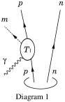
In this study we are interested in the photoproduction of an $\eta^{\prime}n$ bound state with forward proton emission, so we calculate the cross sections by considering kinetically favored amplitudes, which are diagrammatically shown in Fig. 1. Namely, we take into account a single-scattering $\eta^{(\prime)}$ photoproduction on a bound proton and double scatterings with the exchange of $\eta^{(\prime)}$ meson, which is produced on a bound proton in the first step. Since we require a fast proton in the forward direction, we can safely neglect the final-state interaction between proton and neutron. In addition, as we will see later, the $\eta^{\prime}$ exchange is most important, since $\eta^{\prime}$ in the intermediate state goes almost on its mass shell at $M_{X}\approx M_{\eta^{\prime}}+M_{n}$. On the other hand, the $\eta$ exchange is suppressed due to its largely off-shell propagation. This means that exchanges of other mesons such as $\pi$ should be suppressed more. We also note that we do not consider diagrams of $\eta$ and $\eta^{\prime}$ photoproductions on a bound neutron. This is because in this condition the final-state neutron should go in forward direction with large momentum while the final-state proton would be slow and its scattering angle would not be restricted to forward due to the kinematics, which can easily be suppressed by the experimental setup.

Thus, we calculate the scattering amplitude $T_{\gamma d\to Xp}$ as

$$T_{\gamma d\to Xp}=\mathcal{T}_{1}^{(m)}+\mathcal{T}_{2}^{(m)}+\mathcal{T}_{3}^{(m)},$$ (3)

where the subscripts $1$, $2$, and $3$ corresponds to the number of the diagrams in Fig. 1. The expression of each amplitude is obtained in a similar manner to that in Refs. Jido:2009jf ; Jido:2010rx ; YamagataSekihara:2012yv ; Jido:2012cy .

The first term $\mathcal{T}_{1}^{(m)}$, corresponding to the single scattering, is evaluated as

$$\mathcal{T}_{1}^{(m)}=T_{\gamma p\to mp}(W_{2})\times\tilde{\varphi}(\bm{p}_{n}),$$ (4)

with the $s$-wave $\gamma p\to mp$ scattering amplitude $T_{\gamma p\to mp}$ denoted by $T_{1}$ in Fig. 1 and the deuteron wave function in momentum space, $\tilde{\varphi}(\bm{q})$, which is given in the deuteron rest frame. Therefore, for the evaluation of the deuteron wave function $\tilde{\varphi}(\bm{p}_{n})$ we have to calculate the neutron momentum in the final state, $\bm{p}_{n}$, in the laboratory frame. The energy $W_{2}$ is calculated as

$$W_{2}=\sqrt{\left(p_{m}^{\mu}+p_{p}^{\mu}\right)^{2}},$$ (5)

where $p_{m}^{\mu}$ and $p_{p}^{\mu}$ are the momenta of the meson $m$ and proton in the final state, which can be evaluated from the final-state phase space.

The second term $\mathcal{T}_{2}^{(m)}$ corresponds to the double scattering with the $\eta^{\prime}$ exchange and evaluated as

$$\mathcal{T}_{2}^{(m)}= T_{\gamma p\to\eta^{\prime}p}(W_{2}^{\prime})T_{\eta^{\prime}n\to mn}(M_{X})$$

$$\times\int\frac{d^{3}q}{(2\pi)^{3}}\frac{\tilde{\varphi}(\bm{q}+\bm{p}_{p}-\bm{k})}{q^{2}-M_{\eta^{\prime}}^{2}+i\epsilon},$$ (6)

with the $\eta^{\prime}n\to mn$ amplitude $T_{\eta^{\prime}n\to mn}$ denoted by $T_{2}$ in Fig. 1, for which we employ an effective model described in the next subsection, the photon and final-state proton momenta in the laboratory frame $\bm{k}=(0,\,0,\,E_{\gamma}^{\rm lab})$ and $\bm{p}_{p}$, respectively, and an infinitesimal positive value $\epsilon$. The energy $W_{2}^{\prime}$ is approximated as

$$W_{2}^{\prime}\approx\sqrt{M_{p}^{2}+2M_{p}E_{\gamma}^{\rm lab}},$$ (7)

by assuming that the initial-state bound proton is at rest on its mass shell. The energy carried by the exchanged meson, $q^{0}$, should be fixed in appropriate models. In this study, we employ two approaches. The first one is the Watson approach Watson:1953zz , which gives us Jido:2012cy

$$q^{0}=M_{p}+E_{\gamma}^{\rm lab}-p_{p}^{0},$$ (8)

in the laboratory frame. In the second approach, we employ the truncated Faddeev approach as done in Ref. Miyagawa:2012xz , in which we have

$$q^{0}=M_{d}+E_{\gamma}^{\rm lab}-p_{p}^{0}-M_{n}-\frac{|\bm{q}+\bm{p}_{p}-\bm{k}|^{2}}{2M_{n}},$$ (9)

in the laboratory frame. Here we refer to the former (latter) treatment as option A (B). The details are given in Ref. Jido:2012cy .

The third term $\mathcal{T}_{3}^{(m)}$ corresponds to the double scattering with the $\eta$ exchange and is evaluated as

$$\mathcal{T}_{3}^{(m)}= T_{\gamma p\to\eta p}(W_{2}^{\prime})T_{\eta n\to mn}(M_{X})$$

$$\times\int\frac{d^{3}q}{(2\pi)^{3}}\frac{\tilde{\varphi}(\bm{q}+\bm{p}_{p}-\bm{k})}{q^{2}-M_{\eta}^{2}+i\epsilon}.$$ (10)

Here the energy carried by the exchanged meson, $q^{0}$, is fixed in the same manner as in the second term, $\mathcal{T}_{2}^{(m)}$, with the option A (8) or B (9).

In our calculation, both $T_{\gamma p\to\eta p}$ and $T_{\gamma p\to\eta^{\prime}p}$ can be factorized out of the integral because we assume it not to depend on the internal energy nor scattering angle. In a more realistic case, both $T_{\gamma p\to\eta p}$ and $T_{\gamma p\to\eta^{\prime}p}$ depend on them and thus should be in principle inside the integral. Nevertheless, the forward proton emission of this reaction, i.e., the scattering angle of the final-state proton, $\theta_{p}$, being around $0$ degree, indicates that neglecting the angular dependence is enough good as a first-order approximation. On the other hand, the energy $W_{2}^{\prime}$ as a parameter of the amplitudes $T_{\gamma p\to mp}$ can be fixed by assuming that the initial-state bound proton in the first scattering is at rest on its mass shell, as done in Ref. Jido:2009jf .

For the deuteron wave function, we neglect the $d$-wave component and we use a parameterization of the $s$-wave component given by an analytic function Lacombe:1981eg as

$$\tilde{\varphi}(\bm{q})=\sum_{j=1}^{11}\frac{C_{j}}{\bm{q}^{2}+m_{j}^{2}},$$ (11)

with $C_{j}$ and $m_{j}$ determined in Machleidt:2000ge .

II.2 The $\bm{\eta^{\prime}N}$ scattering amplitude

Next we formulate the $\eta^{\prime}N$ scattering amplitude around the $\eta^{\prime}N$ threshold. In this study we consider an $s$-wave $\eta^{\prime}N$-$\eta N$ coupled-channels problem, since the $\eta N$ channel can be important to the $\eta^{\prime}N$ scattering amplitude as the closest open channel in $s$ wave. In this study, we employ the $\eta^{\prime}N$ amplitude obtained from the linear sigma model with unitarization according to the approach developed in Refs. Sakai:2013nba ; Sakai:2014zoa . The scattering amplitude $T_{ij}$ is labeled by the channel indices $i$ and $j$ as $i=1$ ($2$) for $\eta^{\prime}N$ ($\eta N$). Here we note that we employ the physical masses for nucleons to calculate quantities, so the nucleon mass $M_{N}$ is equal to $M_{p}$ for the $\eta^{(\prime)}p$ reaction and to $M_{n}$ for the $\eta^{(\prime)}n$ reaction in the following formulation, while the interaction term is constructed with isospin symmetry.

According to Refs. Sakai:2013nba ; Sakai:2014zoa , we construct an interaction kernel from the linear sigma model as

$$V_{11}=-\frac{6gB}{\sqrt{3}m_{\sigma 0}^{2}},\quad V_{12}=V_{21}=+\frac{6gB}{\sqrt{6}m_{\sigma 8}^{2}},\quad V_{22}=0,$$ (12)

where constants $g$, $B$, $m_{\sigma 0}$, and $m_{\sigma 8}$ determine the strength of the interaction; $g$ is the coupling constant for the $\sigma NN$ vertex, $B$ represents the contribution from the $\text{U}_{\rm A}(1)$ anomaly, and $m_{\sigma 0}$ and $m_{\sigma 8}$ are the masses of the singlet and octet sigma mesons exchanged between $\eta^{(\prime)}$ and $N$. These parameters are fixed as $g=7.67$, $B=0.984\text{ GeV}$, $m_{\sigma 0}=0.7\text{ GeV}$, and $m_{\sigma 8}=1.23\text{ GeV}$ Sakai:2013nba .

Here, we note that the contribution from the $\eta N$ channel is not so large because the mixing angle between the $\eta$ and $\eta^{\prime}$ is small and the transition of the $\eta^{\prime}N$ into $\eta N$ governed by Eq. (12) is suppressed by the large mass of the octet scalar meson $m_{\sigma 8}$. This means that the following result would not depend so much on the details of the treatment of the $\eta N$ channel.

We use this tree-level interaction as an interaction kernel, and solve the scattering equation to obtain the scattering amplitude $T_{ij}(w)$:

$$T_{ij}(w)=V_{ij}+\sum_{k=1}^{2}V_{ik}G_{k}(w)T_{kj}(w),$$ (13)

where $w$ is the center-of-mass energy and $G_{i}$ is the $\eta^{(\prime)}N$ loop function. It is important that the tree-level amplitude $V_{ij}$ is independent of the external momentum [see Eq. (12)], and thus the scattering equation becomes an algebraic equation. For the loop function $G_{i}$, we employ a covariant expression as

$$G_{i}(w)\equiv i\int\frac{d^{4}q}{(2\pi)^{4}}\frac{2M_{N}}{[(P-q)^{2}-M_{N}^{2}](q^{2}-M_{i}^{2})},$$ (14)

with $P^{\mu}=(w,\,\bm{0})$, $M_{1}=M_{\eta^{\prime}}$, and $M_{2}=M_{\eta}$, and the loop function is calculated with the dimensional regularization as

$$G_{i}(w)=\frac{2M_{N}}{16\pi^{2}}\bigg{[}a_{i}(\mu_{\rm reg})+\ln\left(\frac{M_{N}^{2}}{\mu_{\rm reg}^{2}}\right)$$

$$+\frac{w^{2}+M_{i}^{2}-M_{N}^{2}}{2w^{2}}\ln\left(\frac{M_{i}^{2}}{M_{N}^{2}}\right)$$

$$-\frac{\lambda^{1/2}(w^{2},\,M_{N}^{2},\,M_{i}^{2})}{w^{2}}\text{artanh}\left(\frac{\lambda^{1/2}(w^{2},\,M_{N}^{2},\,M_{i}^{2})}{M_{N}^{2}+M_{i}^{2}-w^{2}}\right)\bigg{]},$$ (15)

with the subtraction constant $a_{i}$ at the regularization scale $\mu_{\rm reg}$, which is set as $\mu_{\rm reg}=M_{N}$. In this study they are fixed by the natural renormalization scheme developed in Ref. Hyodo:2008xr so as to exclude the Castillejo-Dalitz-Dyson (CDD) pole contribution from the loop function. This can be achieved by requiring $G_{i}(w=M_{N})=0$ for every channel $i$.

In this construction, a sufficient attraction between $\eta^{\prime}$ and $N$ leads to an $\eta^{\prime}N$ bound state described by a pole of the scattering amplitude $T_{ij}(w)$ with its residue $g_{i}g_{j}$:

$$T_{ij}(w)=\frac{g_{i}g_{j}}{w-w_{\rm pole}}+(\text{regular at }w=w_{\rm pole}).$$ (16)

The residue $g_{i}$ can be interpreted as the coupling constant of the $\eta^{\prime}N$ bound state to the $i$ channel. The coupling constant $g_{i}$ is further translated into the so-called compositeness $X_{i}$ via the two-body wave function so as to measure the fraction of the two-body component Hyodo:2011qc ; Aceti:2012dd ; Hyodo:2013nka ; Sekihara:2014kya ; Sekihara:2015gvw . Namely, in the present formulation the two-body wave function in channel $i$ in momentum space $\tilde{\Psi}_{i}(\bm{q})$ is proportional to the coupling constant $g_{i}$ Gamermann:2009uq ; YamagataSekihara:2010pj as

$$\tilde{\Psi}_{i}(\bm{q})=\frac{g_{i}\sqrt{4M_{N}w_{\rm pole}}}{w_{\rm pole}^{2}-[\omega_{i}(\bm{q})+\Omega_{N}(\bm{q})]^{2}}.$$ (17)

Then, the compositeness is defined as the norm of $\tilde{\Psi}_{i}(\bm{q})$, and its expression is

$$X_{i}= \int\frac{d^{3}q}{(2\pi)^{3}}\frac{\omega_{i}(\bm{q})+\Omega_{N}(\bm{q})}{2\omega_{i}(\bm{q})\Omega_{N}(\bm{q})}\left[\tilde{\Psi}_{i}(\bm{q})\right]^{2}$$

$$= -g_{i}^{2}\frac{dG_{i}}{dw}(w=w_{\rm pole}),$$ (18)

where $\omega_{i}(\bm{q})\equiv\sqrt{M_{i}^{2}+\bm{q}^{2}}$ and $\Omega_{N}(\bm{q})\equiv\sqrt{M_{N}^{2}+\bm{q}^{2}}$. Here we note that the compositeness as well as the wave function is a scheme dependent quantity, i.e., we can uniquely determine it when we fix the model space, interaction, and loop function. Since we take into account only the $\eta^{\prime}N$ and $\eta N$ channels in the present model, the sum of the norms for the $\eta^{\prime}N$ and $\eta N$ channels, $X_{1}+X_{2}$, coincides with the normalization of the total bound-state wave function $|\Psi\rangle$ as

$$\langle\Psi^{\ast}|\Psi\rangle=X_{1}+X_{2}=1.$$ (19)

In this sense, one can deduce the structure by comparing the value of the compositeness with unity. Besides, we may take into account missing channels, which do not appear as explicit degrees of freedom in the model space, by employing an energy dependent two-body interaction, as such a missing channel inevitably brings energy dependence to the two-body interaction Sekihara:2014kya ; Hyodo:2008xr .

Table 1: Pole position $w_{\rm pole}$, coupling constant $g_{i}$ ($i=\eta^{\prime}N$, $\eta N$), and compositeness $X_{i}$ of the $\eta^{\prime}N$ bound state in the present model.

$w_{\rm pole}$ [MeV]	$1889.5-6.3i$
$g_{\eta^{\prime}N}$	$2.40+0.45i$
$g_{\eta N}$	$-0.54-0.07i\phantom{-}$
$X_{\eta^{\prime}N}$	$1.01+0.00i$
$X_{\eta N}$	$-0.01+0.00i\phantom{-}$

The values of the pole position, coupling constant, and compositeness of the $\eta^{\prime}N$ bound state in the present model are listed in Table 1. As one can see, the pole position $w_{\rm pole}$ has a small imaginary part as a decay of the $\eta^{\prime}N$ bound state to the $\eta N$ channel, and the value is consistent with the experimental implication in Ref. Moyssides:1983 . The modulus of the $\eta^{\prime}N$ coupling constant is about five times larger than that of the $\eta N$ one. Since the $\eta^{\prime}N$ compositeness $X_{\eta^{\prime}N}$ is close to unity with a negligible imaginary part, the $\eta^{\prime}N$ bound state in the present model parameter is indeed dominated by the $\eta^{\prime}N$ component.

II.3 The $\bm{\gamma p\to\eta p}$ and $\bm{\eta^{\prime}p}$ scattering amplitudes

Figure 2: Feynman diagrams for the $\gamma p\to mp$ reaction with $m=\eta$ or $\eta^{\prime}$. Here the solid, dashed, and wavy lines represent the proton, $m$, and photon, respectively. The open and shaded circles correspond to the $\gamma p\to mp$ and $mp\to mp$ amplitudes, respectively.

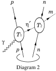
Finally, let us consider photoproductions of $\eta$ and $\eta^{\prime}$ on a proton target. In this study, we introduce the rescattering of $\eta^{(\prime)}p$ in the final state of the $\gamma p\to mp$ reaction with $m=\eta$ or $\eta^{\prime}$, as done in Ref. Nacher:1998mi . Namely, with the $\eta^{(\prime)}N\to\eta^{(\prime)}N$ amplitude developed in the previous subsection, we construct the scattering amplitude $T_{\gamma p\to mp}$ in the approach diagrammatically shown in Fig. 2, which is expressed as

$$T_{\gamma p\to i}(W)=V_{\gamma i}+\sum_{j=1}^{2}V_{\gamma j}G_{j}(W)T_{ji}(W).$$ (20)

Here $W$ is the center-of-mass energy, $T_{ji}$ and $G_{j}$ are the $\eta^{(\prime)}p\to\eta^{(\prime)}p$ scattering amplitude and loop function developed in the previous subsection, respectively, and the channel index $i=1$ ($2$) indicates the $\eta^{\prime}p$ ($\eta p$) channel. In general we may take different subtraction constants for the loop functions $G_{i}$ in Eqs. (13) and (20), but the same subtraction constant is used in this study. In contrast, the $\gamma p\to i$ part $V_{\gamma i}$ is unknown model parameter.

Figure 3: Differential cross sections of $\gamma p\to\eta p$ and $\eta^{\prime}p$ reactions calculated with the amplitudes in Eq. (20) and comparison with the experimental data in Refs. Williams:2009yj ; Sumihama:2009gf . The experimental data are taken with the scattering angle $-0.8<\cos\theta_{m}^{\rm cm}<-0.7$ for both $\eta$ and $\eta^{\prime}$ photoproductions with $\theta_{m}^{\rm cm}$ being the meson angle in the center-of-mass frame.

In this study we fix $V_{\gamma p\to i}$ by using the experimental data of the differential cross section for the reaction $\gamma p\to mp$, which is expressed as

$$\frac{d\sigma_{\gamma p\to mp}}{d\Omega}=\frac{p_{\rm cm}^{\prime}M_{p}}{16\pi^{2}E_{\gamma}^{\rm lab}W}|T_{\gamma p\to mp}|^{2}.$$ (21)

Here $\Omega$ is the solid angle for the momentum of the final-state proton in the center-of-mass frame and the total energy $W$ is obtained as $W=\sqrt{M_{p}^{2}+2M_{p}E_{\gamma}^{\rm lab}}$. The magnitude of the momentum of the final-state proton in the center-of-mass frame, $p_{\rm cm}^{\prime}$, can be calculated as

$$p_{\rm cm}^{\prime}=\frac{\lambda^{1/2}(W^{2},\,M_{p}^{2},\,M_{m}^{2})}{2W}.$$ (22)

Here we note that, since we mainly concentrate on the forward proton emission, we may need only the scattering amplitude at a certain angle. Furthermore, in this study we are interested in the ratio of the $\eta^{\prime}n$ bound state signal to the $\eta^{\prime}$ quasifree contribution. In this sense, regarding the $\gamma p\to i$ part $V_{\gamma i}$ to be constant is enough for our purpose to calculate the relative strength between the $\eta^{\prime}n$ bound state signal and the $\eta^{\prime}$ quasifree contribution in the forward proton emission. Thus, we fix two fitting parameters $V_{\gamma 1}$ and $V_{\gamma 2}$ so as to reproduce the experimental data. For the forward proton emission, we use the experimental data on the $\gamma p\to\eta^{\prime}p$ and $\eta p$ reactions in the scattering angle $-0.8<\cos\theta_{m}^{\rm cm}<-0.7$ with the $\eta^{(\prime)}$ scattering angle $\theta_{m}^{\rm cm}$ Williams:2009yj ; Sumihama:2009gf . As we will see in the numerical results, the $\gamma p\to\eta^{\prime}p$ reaction is most important, so we give more weight to the data of the $\gamma p\to\eta^{\prime}p$ reaction. From the fit with the parameters in the $\eta^{(\prime)}N\to\eta^{(\prime)}N$ amplitude ($g=7.67$, $B=0.984\text{ GeV}$, $m_{\sigma 0}=0.7\text{ GeV}$, and $m_{\sigma 8}=1.23\text{ GeV}$), we take the following parameters:

$$V_{\gamma 1}=0.348\text{ GeV}^{-1},\quad V_{\gamma 2}=0.354\text{ GeV}^{-1},$$ (23)

which reproduce the experimental cross sections with forward proton emission above the $\eta^{\prime}p$ threshold in Ref. Williams:2009yj ; Sumihama:2009gf , as shown in Fig. 3. We note that in Fig. 3 we have a prominent peak in the $\gamma p\to\eta p$ cross section below $W=1.9\text{ GeV}$ corresponding to the signal of the $\eta^{\prime}p$ bound state. In actual experimental observation, this contribution should interfere with others coming from the nonresonant background. This may provide a peak structure or a dip, generally a Fano resonance, depending on the interference.

We emphasize again that this strategy is sufficient for our purpose to estimate the production ratio of the $\eta^{\prime}n$ bound state compared to the $\eta^{\prime}$ quasifree contributions with forward proton emission. Actually, around the $\eta^{\prime}n$ threshold the strength of both the bound state signal and the quasifree contribution is similarly suppressed as the scattering angle increases, and hence a large cancellation will take place when we take the signal to quasifree ratio.

III Numerical Results

Now we calculate the differential cross section (1) for the $\gamma d\to mnp$ reaction with $m=\eta$ or $\eta^{\prime}$. We first perform theoretical studies of the signal for the $\eta^{\prime}n$ bound state in the photoproduction process in Sec. III.1. In this section, after examining two options, i.e., the Watson approach (8) and the truncated Faddeev approach (9), we investigate each diagram contribution to the cross sections of the two reactions. In addition, we study how the signal of the $\eta^{\prime}n$ bound state depends on the strength of the $\eta^{\prime}N$ interaction. Then, in Sec. III.2 we discuss how the signal of the $\eta^{\prime}n$ bound state can be seen in several experimental conditions. We here show the dependence of our results with respect to the initial photon energy and the scattering angle of the final-state proton, and integrate the differential cross section with respect to the scattering angle for the forward proton emission.

Throughout this section, the initial photon energy $E_{\gamma}^{\rm lab}$ and proton scattering angle in the global center-of-mass frame $\theta_{p}^{\rm cm}$ are fixed as $E_{\gamma}^{\rm lab}=2.1\text{ GeV}$ and $\theta_{p}^{\rm cm}=0$ degree, respectively, unless explicitly mentioned.

III.1 Theoretical study of the $\bm{\eta^{\prime}n}$ signal

III.1.1 Signal of the $\eta^{\prime}n$ bound state in two options

Figure 4: Invariant mass spectra for the $\gamma d\to Xp$ reactions with $X=\eta n$ and $\eta^{\prime}n$. The exchanged meson energy $q^{0}$ is fixed as in Eq. (8) [Eq. (9)] for the option A (B). The initial photon energy is fixed as $E_{\gamma}^{\rm lab}=2.1\text{ GeV}$ and the proton scattering angle in the global center-of-mass is $\theta_{p}^{\rm cm}=0$ degree.

First of all, we examine two options of the exchanged meson energy: A for the Watson approach (8) and B for the truncated Faddeev approach (9). We calculate the differential cross sections for the $\gamma d\to\eta np$ and $\eta^{\prime}np$ reactions in both two approaches as functions of the invariant mass $M_{X}=M_{\eta n}$ and $M_{\eta^{\prime}n}$, and the result is shown in Fig. 4 in the range [$1.86\text{ GeV}$, $1.94\text{ GeV}$]. As one can see from the figure, in both options A and B, we can clearly observe the signal of the $\eta^{\prime}n$ bound state in the $\eta n$ mass spectrum below the $\eta^{\prime}n$ threshold $\approx 1.897\text{ GeV}$, which is comparable to the quasifree $\eta^{\prime}$ contribution in the $\eta^{\prime}n$ mass spectrum above the threshold. However, the strength of the bound state signal is different in two options, while very similar quasifree $\eta^{\prime}$ contributions are found. Namely, the option A (B) gives a larger (smaller) signal of the $\eta^{\prime}n$ bound state. This difference could be interpreted as a theoretical ambiguity in calculating the differential cross section of the $\gamma d$ reaction in the present formulation.

Here we should mention that in the option A we have a small cusp in the $\eta n$ spectrum around $1.88\text{ GeV}$, which is an artificial threshold in the Watson approach Miyagawa:2012xz ; Jido:2012cy . Since we are interested in the signal of the $\eta^{\prime}n$ bound state in clearer conditions, we employ only the option B, which gives smaller signal of the bound state, in the following calculations.

Let us now numerically compare the contributions from the bound state signal and from others above the $\eta^{\prime}n$ threshold in option B. This can be achieved by integrating the differential cross section in appropriate ranges of the invariant mass $M_{X}$. On the one hand, the signal contribution is obtained by integrating $d^{2}\sigma_{\gamma d\to\eta np}/dM_{X}d\Omega_{p}$ in the range $[1.86\text{ GeV},\,M_{\eta^{\prime}}+M_{n}]$, which results in $0.011~{}\mu\text{b}/\text{sr}$. On the other hand, the other contributions above the $\eta^{\prime}n$ threshold contains the quasifree $\eta^{\prime}$ in the $\eta^{\prime}n$ spectrum and the tail of the $\eta^{\prime}n$ bound state signal in the $\eta n$ spectrum. Thus, we integrate the sum of the cross section in the two reactions, $d^{2}\sigma_{\gamma d\to\eta np}/dM_{X}d\Omega_{p}+d^{2}\sigma_{\gamma d\to\eta^{\prime}np}/dM_{X}d\Omega_{p}$, in the range $[M_{\eta^{\prime}}+M_{n},\,2.0\text{ GeV}]$, which results in $0.055~{}\mu\text{b}/\text{sr}$. Therefore, we obtain the ratio of the signal to other contributions as $0.011/0.055=0.20$.

III.1.2 Contribution from each diagram

Figure 5: Invariant mass spectrum for the $\gamma d\to\eta np$ reaction. The initial photon energy is fixed as $E_{\gamma}^{\rm lab}=2.1\text{ GeV}$ and the proton scattering angle in the global center-of-mass is $\theta_{p}^{\rm cm}=0$ degree. The inset represents an enlarged figure.

Next, we show in Fig. 5 the numerical result of each diagram contribution to the differential cross section for the $\gamma d\to\eta np$ reaction (1) as a function of the invariant mass $M_{X}=M_{\eta n}$. As one can see, we observe that in this invariant mass region the cross section is dominated by the diagram 2 in Fig. 1, i.e., the $\eta^{\prime}$ exchange contribution. This is because the invariant mass in this region contains the $\eta^{\prime}n$ threshold and thus the exchanged $\eta^{\prime}$ can go almost on its mass shell to generate an $\eta^{\prime}n$ bound state. On the other hand, both the diagrams 1 and 3 in Fig 1 are negligible. The contribution from the single scattering (diagram 1) is strongly suppressed by the deuteron wave function. Namely, in order to make the $\eta n$ invariant mass as large as the $\eta^{\prime}n$ threshold energy with the forward proton emission only by the single scattering, we need anomalously large Fermi motion of a bound neutron in the forward direction. The $\eta$ exchange as the diagram 3 is also small because the exchanged $\eta$ cannot approach on its mass shell in the $\eta^{\prime}n$ bound region with forward proton emission and the magnitude of the $\eta n\to\eta n$ amplitude is small compared to that of the $\eta^{\prime}n\to\eta n$ one employed in the diagram 2.

Figure 6: Invariant mass spectrum for the $\gamma d\to\eta^{\prime}np$ reaction. The initial photon energy is fixed as $E_{\gamma}^{\rm lab}=2.1\text{ GeV}$ and the proton scattering angle in the global center-of-mass is $\theta_{p}^{\rm cm}=0$ degree. The inset represents an enlarged figure.

In Fig. 6, we show the numerical result of the differential cross section for the $\gamma d\to\eta^{\prime}np$ reaction around the $\eta^{\prime}n$ threshold. The cross section starts at the $\eta^{\prime}n$ threshold. From the figure, we find that the quasifree $\eta^{\prime}$ contribution in the single scattering (diagram 1 in Fig. 1) dominates the cross section. This is caused by the deuteron wave function; since a bound proton and a bound neutron are almost at rest inside a deuteron, the $\eta^{\prime}$ meson produced by the $\gamma p^{\ast}\to\eta^{\prime}p$ reaction with a bound proton $p^{\ast}$ should be slow if the final-state proton goes the forward angle with $\theta_{p}^{\rm cm}=0$ degree, which makes the invariant mass $M_{X}$ to be close to the $\eta^{\prime}n$ threshold. Besides, the tail of an $\eta^{\prime}n$ bound state peak can make the $\eta^{\prime}$ exchange diagram (diagram 2) be a nonnegligible contribution to the cross section as the dashed-dotted line in Fig. 6. On the other hand, the $\eta$ exchange diagram negligibly contribute to the cross section due to a similar reason as in the $\gamma d\to\eta np$ reaction.

An interesting point is that we can observe the destructive interference between the quasifree $\eta^{\prime}$ photoproduction of the single scattering and the $\eta^{\prime}$ exchange contribution. This means the absorption of $\eta^{\prime}$ produced on a bound proton into the bound neutron inside the same deuteron. Actually, we can easily find that double scattering amplitude constructed with the imaginary part of the $\eta^{\prime}n\to\eta^{\prime}n$ amplitude and the on-shell $\eta^{\prime}$ exchange has opposite sign compared to the single scattering one. The present result provides us with an expectation that one may extract information on the $\eta^{\prime}N$ interaction from the quasifree $\eta^{\prime}$ production yield on a deuteron target compared to that on a proton target. We also expect large medium effects for $\eta^{\prime}$ such as the transparency ratio even in light nuclei.

III.1.3 Dependence on the strength of the $\eta^{\prime}N$ interaction

Table 2: Properties of the $\eta^{\prime}n$ bound state with several values of the parameter $g$ or $m_{\sigma 8}$. When changing the value of the parameter $g$ or $m_{\sigma 8}$, other parameters remain fixed. We also consider the case that we introduce the contribution from the $\pi N$ channel Sakai:2016 . the The binding energy $B_{\rm E}$ and width $\Gamma$ are defined as $B_{\rm E}\equiv M_{\eta^{\prime}}+M_{n}-\text{Re}\,w_{\rm pole}$ and $\Gamma\equiv-2\,\text{Im}\,w_{\rm pole}$, respectively.

Shift parameter $g$
$g$	$g_{\eta^{\prime}n}$	$B_{\rm E}$ [MeV]	$\Gamma$ [MeV]
$5.0$	No structure
$6.0$	Cusp only
$7.0$	$1.63+0.56i$	$0.9$	$5.4$
$8.0$	$2.71+0.43i$	$12.8\phantom{0}$	$16.0\phantom{0}$
$9.0$	$3.49+0.40i$	$31.8\phantom{0}$	$26.0\phantom{0}$
Shift parameter $m_{\sigma 8}$
$m_{\sigma 8}$ [GeV]	$g_{\eta^{\prime}n}$	$B_{\rm E}$ [MeV]	$\Gamma$ [MeV]
$0.9$	$3.19+1.25i$	$9.5$	$60.9\phantom{0}$
$1.0$	$2.79+0.91i$	$8.8$	$34.4\phantom{0}$
$1.1$	$2.57+0.67i$	$8.4$	$21.2\phantom{0}$
$1.2$	$2.43+0.49i$	$8.0$	$14.1\phantom{0}$
$1.3$	$2.34+0.37i$	$7.7$	$9.8$
Introduce $\pi N$ channel
	$g_{\eta^{\prime}n}$	$B_{\rm E}$ [MeV]	$\Gamma$ [MeV]
	$4.10+0.15i$	$57.0$	$14.5$

Now we see the dependence on the strength of the $\eta^{\prime}n$ interaction for the peak structure of the $\eta^{\prime}n$ bound state in the $\gamma d\to pX$ reaction with $X=\eta n$ and $\eta^{\prime}n$. Here we vary the interaction strength via the model parameter $g$ or $m_{\sigma 8}$ in the interaction kernel (12), and by introducing the contribution from the $\pi N$ channel. Since we are interested in how the signal of the $\eta^{\prime}n$ bound state depends on the model parameters, we modify the interaction strength only for the second scattering, i.e., $T_{2}$ in Fig. 1, while we fix the first step of the reaction ($T_{1}$ in Fig. 1) unchanged. We note that when we change the value of the parameter $g$ or $m_{\sigma 8}$, other parameters remain fixed as their original values.

Figure 7: Invariant mass spectrum for the $\gamma d\to Xp$ reaction with $X=\eta n$ and $\eta^{\prime}n$ as the sum of the two contributions. The interaction strength is controlled by the parameter $g$ in Eq. (12). The initial photon energy is fixed as $E_{\gamma}^{\rm lab}=2.1\text{ GeV}$ and the proton scattering angle in the global center-of-mass is $\theta_{p}^{\rm cm}=0$ degree.

Figure 8: Invariant mass spectrum for the $\gamma d\to\eta^{\prime}np$ reaction. The interaction strength is controlled by the parameter $g$ in Eq. (12). The initial photon energy is fixed as $E_{\gamma}^{\rm lab}=2.1\text{ GeV}$ and the proton scattering angle in the global center-of-mass is $\theta_{p}^{\rm cm}=0$ degree.

First we vary the interaction strength via $g$, which is the coupling constant for the $\sigma NN$ vertex. Since the coupling constant $g$ is commonly introduced to the $\eta^{\prime}n\leftrightarrow\eta^{\prime}n$ and $\eta^{\prime}n\leftrightarrow\eta n$ interaction, as the value of $g$ becomes large both the binding energy $B_{\rm E}\equiv M_{\eta^{\prime}}+M_{n}-\text{Re}\,w_{\rm pole}$ and width $\Gamma\equiv-2\,\text{Im}\,w_{\rm pole}$ of the $\eta^{\prime}n$ bound state increase. We show in the upper panel of Table 2 the properties of the $\eta^{\prime}n$ bound state with several values of $g$. We have checked that in the present condition the coupling constant $g\geq 6.9$ can form an $\eta^{\prime}n$ bound state below the $\eta^{\prime}n$ threshold.

The behavior of the signal of the $\eta^{\prime}n$ bound state is shown in Fig. 7, where we plot the sum of the differential cross sections of $\gamma d\to\eta np$ and $\eta^{\prime}np$ with the parameter $g=5.0$ to $9.0$ in intervals of $1.0$. From the figure, we can clearly observe the signal of the $\eta^{\prime}n$ bound state for $g=7.0$ and $8.0$. However, for $g=9.0$, the signal of the bound state becomes weak due to its large decay width, $\Gamma=26.0\text{ MeV}$. In addition, for $g=6.0$, we find only a cusp structure at the $\eta^{\prime}n$ threshold, as the interaction with $g=6.0$ cannot bind the $\eta^{\prime}n$ system below the $\eta^{\prime}n$ threshold. Such a cusp structure disappears when we take $g=5.0$. This result indicates that, if the $\eta^{\prime}N$ interaction is attractive enough, we have a chance to observe some peculiar structure around the $\eta^{\prime}n$ threshold, i.e., the bound state signal ($g=7.0$, $8.0$ and $9.0$) or a cusp of the differential cross section at the $\eta^{\prime}n$ threshold ($g=6.0$). We also note that we may observe interesting behavior in the $\eta^{\prime}n$ invariant mass spectrum just above its threshold, which reflects the physics below the $\eta^{\prime}n$ threshold, as seen in Fig. 8, where we plot only the $\eta^{\prime}n$ invariant mass spectrum. In the present model, one finds that the $\eta^{\prime}n$ invariant mass spectrum is convex downward just above the $\eta^{\prime}n$ threshold for $g>6$, in which there is a bound state below the threshold, while it turns to be convex upward for $g\leq 6$, where there is no bound state.

Figure 9: Invariant mass spectrum for the $\gamma d\to Xp$ reaction with $X=\eta n$ and $\eta^{\prime}n$ as the sum of the two contributions. The interaction strength is controlled by the parameter $m_{\sigma 8}$ in Eq. (12). The initial photon energy is fixed as $E_{\gamma}^{\rm lab}=2.1\text{ GeV}$ and the proton scattering angle in the global center-of-mass is $\theta_{p}^{\rm cm}=0$ degree.

Next, we shift the value of the parameter $m_{\sigma 8}$, which is the mass of the octet $\sigma$ meson exchanged between $\eta^{(\prime)}$ and $n$. Since $m_{\sigma 8}$ determines the strength of the transition $\eta^{\prime}N\leftrightarrow\eta N$, this mainly controls the decay width of the $\eta^{\prime}n$ bound state; the smaller value of $m_{\sigma 8}$ brings the larger decay width of the $\eta^{\prime}n$ bound state with a similar binding energy. The properties of the $\eta^{\prime}n$ bound state are listed in the middle panel of Table 2.

By changing the value of $m_{\sigma 8}$, we can study how the bound state signal melts with large decay width in the differential cross section. In Fig. 9 we show our result of the sum of the differential cross sections of $\gamma d\to\eta np$ and $\eta^{\prime}np$ with the parameter $m_{\sigma 8}=0.9\text{ GeV}$ to $1.3\text{ GeV}$ in intervals of $0.1\text{ GeV}$. We can see from Fig. 9 that for $m_{\sigma 8}\geq 1.1\text{ GeV}$ the signal of the $\eta^{\prime}n$ bound state is clear and nonnegligible compared to the quasifree contribution above the $\eta^{\prime}n$ threshold. In contrast, for $m_{\sigma 8}\leq 1.0\text{ GeV}$, we have only negligible contribution of the bound state signal. This result indicates that, even if there would exist an $\eta^{\prime}n$ bound state, we could not see its signal in the $\gamma d\to pn\eta$ reaction if its decay width is $\Gamma\gtrsim 25\text{ MeV}$.

Figure 10: Invariant mass spectrum for the $\gamma d\to Xp$ reaction with $X=\eta n$ and $\eta^{\prime}n$ as the sum of the two contributions. Solid and dashed lines represent the invariant mass spectra with and without inclusion of the $\pi N$ channel, respectively. The initial photon energy is fixed as $E_{\gamma}^{\rm lab}=2.1\text{ GeV}$ and the proton scattering angle in the global center-of-mass is $\theta_{p}^{\rm cm}=0$ degree.

Finally, we introduce the contribution from the $\pi N$ channel to the $\eta^{\prime}N$ interaction in the linear sigma model. The contribution from the $\pi N$ channel is included in order to respect the experimental data given in Ref. Rader:1973mx . Within this treatment, the effect of the coupling with $\pi N$ channel would not be so significant. Besides, for a more realistic treatment of the model, we also take into account the effect of the flavor SU(3) symmetry breaking. This SU(3) symmetry breaking makes the $\sigma_{0}$ mass lighter. As a result, the interaction in the $\eta^{\prime}N$ elastic channel, which contains $m_{\sigma 0}$ in the denominator, becomes more attractive and hence the binding energy of the $\eta^{\prime}N$ system increases. In the present model, the binding energy of the $\eta^{\prime}N$ bound state grows to $57.0\text{ MeV}$, which can be interpreted as a model parameter $m_{\sigma 0}$ dependence, but its decay width is still narrow, $14.5\text{ MeV}$. The details are given in Ref. Sakai:2016 . We note that, in the calculation of the reaction cross sections, we do not take into account the double scattering amplitude with the $\pi$ exchange, since the exchanged $\pi$ should go far from its mass shell, which gives only a negligible contribution.

We show in Fig. 10 the result of the sum of the differential cross sections of $\gamma d\to\eta np$ and $\eta^{\prime}np$. From the figure we can observe a clear signal of the $\eta^{\prime}n$ bound state at $M_{X}=1.84\text{ GeV}$ though the peak of the bound-state signal is reduced compared with that without $\pi N$ channel.

III.2 Behavior of the signal of the $\bm{\eta^{\prime}n}$ bound state in several experimental conditions

Let us now discuss how the signal of the $\eta^{\prime}n$ bound state can be seen in several experimental conditions. The model parameters are the same as those given in Sec. II.

III.2.1 Photon energy dependence

Figure 11: Invariant mass spectrum for the $\gamma d\to Xp$ reaction with $X=\eta n$ and $\eta^{\prime}n$ as the sum of the two contributions. The initial photon energy is taken from $E_{\gamma}^{\rm lab}=2.0\text{ GeV}$ to $2.4\text{ GeV}$ in intervals of $0.1\text{ GeV}$. The proton scattering angle in the global center-of-mass is $\theta_{p}^{\rm cm}=0$ degree.

First we examine the initial photon energy dependence of the differential cross section. We take the initial photon energy from $E_{\gamma}^{\rm lab}=2.0\text{ GeV}$ to $2.4\text{ GeV}$ in intervals of $0.1\text{ GeV}$ and the proton scattering angle $\theta_{p}^{\rm cm}=0$ degree. The result of the cross section around the $\eta^{\prime}n$ threshold is plotted in Fig. 11.

From Fig. 11, we can find that the peak height of the signal of the $\eta^{\prime}n$ bound state at $1.89\text{ GeV}$ is almost unchanged as the initial photon energy increases. This is due to the two facts on the $\eta^{\prime}$ photoproduction. First, the $\gamma p\to\eta^{\prime}p$ reaction cross section, and hence its amplitude, decreases as the photon energy increases, as seen in Fig. 3. Second, with forward proton emission, $\eta^{\prime}$ produced on a bound proton becomes slower in the laboratory frame as the photon energy increases, which makes the intermediate $\eta^{\prime}$ close to on its mass shell in the $\eta^{\prime}n$ signal region, and hence the $\eta^{\prime}$ exchange contribution becomes stronger. These two contributions compensate each other, and as a result the signal of the bound state is almost unchanged regardless of the initial photon energy. On the other hand, while the peak height of the $\eta^{\prime}$ quasifree contribution seen above the $\eta^{\prime}n$ threshold is similar, its peak position shifts downward as the photon energy increases. This is caused by that $\eta^{\prime}$ produced on a bound proton becomes slower in the laboratory frame as the photon energy increases, which makes the $\eta^{\prime}n$ invariant mass lower.

III.2.2 Scattering angle dependence

Figure 12: Invariant mass spectrum for the $\gamma d\to Xp$ reaction with $X=\eta n$ and $\eta^{\prime}n$ as the sum of the two contributions. The scattering angle of the final-state proton is taken from $\theta_{p}^{\rm cm}=0$ to $30$ degrees in the global center-of-mass frame. The initial photon energy is fixed as $E_{\gamma}^{\rm lab}=2.1\text{ GeV}$.

Next, we change the value of the scattering angle of the final-state proton. Here we take the scattering angle in the global center-of-mass frame, $\theta_{p}^{\rm cm}$, from $0$ to $30$ degrees in intervals of $10$ degrees. The result of the differential cross section in these values of the scattering angle is shown in Fig. 12. From the figure, for larger scattering angle $\theta_{p}^{\rm cm}$, we observe smaller bound state signal. This is because, with finite $\theta_{p}^{\rm cm}$, exchanged $\eta^{\prime}$ goes largely off-shell due to a large transverse momentum and hence the $\eta^{\prime}$ exchange contribution becomes weak. Therefore, this result indicates that the forward proton emission is suitable for the production of the $\eta^{\prime}n$ bound state, as we have expected. However, we also see that the quasifree $\eta^{\prime}$ peak shifts upward due to the same kinematics. This fact may help us to observe the signal of the $\eta^{\prime}n$ bound state in actual experiments, as in experiments we measure the production cross sections with finite scattering angles.

III.2.3 Integrating the angle for forward proton emission

Figure 13: Invariant mass spectrum for the $\gamma d\to Xp$ reaction with $X=\eta n$ and $\eta^{\prime}n$ as the sum of the two contributions. The scattering angle of the final-state proton in the laboratory frame, $\theta_{p}^{\rm lab}$, is integrated in the ranges [$0^{\circ}$, $5^{\circ}$], [$0^{\circ}$, $10^{\circ}$], and [$0^{\circ}$, $20^{\circ}$]. The initial photon energy is fixed as $E_{\gamma}^{\rm lab}=2.1\text{ GeV}$.

Finally, in order to see the cross section corresponding to the realistic experimental observations, we show the cross section integrated with respect to the scattering angle for forward proton emission in the laboratory frame in Fig. 13. The result indicates that, in any cases of the upper limit of the scattering angle, we can clearly distinguish the signal of the $\eta^{\prime}n$ bound state, if existed, from the $\eta^{\prime}$ quasifree contribution. This result indicates that we will observe the signal of the $\eta^{\prime}n$ bound state in experiments of the $\gamma d\to\eta^{(\prime)}np$ reaction with forward proton emission, especially if the bound state exists at more than several MeV below the $\eta^{\prime}n$ threshold with a small decay width.

IV Conclusion

In this study, we have investigated possibilities of observing a signal of an $\eta^{\prime}n$ bound state in the photoproductions of the $\eta$ and $\eta^{\prime}$ mesons on a deuteron target with forward proton emission. For this purpose, we have described the production process by two portions. One is the photoproduction of the $\eta^{(\prime)}$ meson on a proton, and the other is the $\eta^{(\prime)}n\to\eta^{(\prime)}n$ scattering. In this study, the $\eta^{(\prime)}N\to\eta^{(\prime)}N$ interaction is obtained in the linear sigma model, and this interaction is employed as a kernel of the scattering equation so as to calculate the $s$-wave $\eta^{(\prime)}N$ scattering amplitude, in which an $\eta^{\prime}N$ bound state can be dynamically generated. On the other hand, the $\gamma p\to\eta p$ and $\eta^{\prime}p$ scattering amplitudes are fixed in an effective model so as to reproduce the experimental cross sections with forward proton emission.

By using these two portions, we have calculated cross sections of the $\gamma d\to\eta np$ and $\eta^{\prime}np$ reactions with forward proton emission in single and $\eta^{(\prime)}$-exchange double scattering processes. As a result, we have found that the signal of the $\eta^{\prime}n$ bound state can be seen below the $\eta^{\prime}n$ threshold in the $\eta n$ invariant mass spectrum of the $\gamma d\to\eta np$ reaction and its strength is comparable with the contribution from the quasifree $\eta^{\prime}$ production above the $\eta^{\prime}n$ threshold in the $\eta^{\prime}n$ invariant mass spectrum. We have found that the double scattering process of the $\eta^{\prime}$ exchange dominates the production of the $\eta^{\prime}n$ bound state. We have also seen a nonnegligible destructive interference between the $\eta^{\prime}$ quasifree contribution in the single scattering and the tail of an $\eta^{\prime}n$ bound state peak coming from the double scattering of the $\eta^{\prime}$ exchange, due to the $\eta^{\prime}$ absorption into the bound neutron. Changing the strength of the $\eta^{\prime}n$ interaction, we have obtained a clear signal of the $\eta^{\prime}n$ bound state if its decay width is about $10\text{ MeV}$. In considering realistic experimental conditions such as several initial photon energy and scattering angle, we have concluded that we will observe the signal of the $\eta^{\prime}n$ bound state in experiments of the $\gamma d\to\eta^{(\prime)}np$ reaction with forward proton emission, especially in the case that the bound state exists at more than several MeV below the $\eta^{\prime}n$ threshold with a small decay width.