Generation of chiral spin state by quantum simulation

Abstract

Chirality of materials in nature appears when there are asymmetries in their lattice structures or interactions in a certain environment. Recent development of quantum simulation technology has enabled the manipulation of qubits. Accordingly, chirality can be realized intentionally rather than passively observed. Here we theoretically provide simple methods to create a chiral spin state in a spin-1/2 qubit system on a square lattice. First, we show that switching ON/OFF the Heisenberg and $XY$ interactions produces the chiral interaction directly in the effective Hamiltonian without controlling local fields. Moreover, when initial states of spin-qubits are appropriately prepared, we prove that the chirality with desirable phase is dynamically obtained. Finally, even for the case where switching ON/OFF the interactions is infeasible and the interactions are always-on, we show that, by preparing an asymmetric initial qubit state, the chirality whose phase is $\pi/2$ is dynamically generated.

I Introduction

Chirality specifies the properties of materials in which the mirror image does not coincide with itself by simple rotations and translations Rikken . Recently, chirality has come to play an important role in the stabilization of skyrmions Nagaosa ; tokura , and, in spintronic devices, chirality is observed in the domain wall motion through the Dzyaloshinsky-Moriya interaction Parkin ; Emori . When the chirality of a spin system supports a nonlocal extension of the order parameter, it is called a chiral spin liquid (CSL) that has attracted much attention in the research of high $T_{\rm c}$ superconductors since the 1980’s Wen ; Wilczek ; WWZ ; Affleck ; Kapitulnik . The research of CSL has been developed in combination with topological quantum computation  YK ; Yao .

The chiral spin state is represented by the chiral interaction $\vec{S}_{i}\cdot\vec{S}_{j}\times\vec{S}_{k}$ ($i,j,k$ indicate lattice sites) WWZ . In the Hubbard model, which can abstract the nature of strongly-correlated electrons, the chiral interactions appear only in the higher order of $t/U$-expansion, and are much smaller than the major Heisenberg couplings $\vec{S}_{i}\cdot\vec{S}_{j}$ Sen . Numerical studies Meng ; Motrunich showed the spin-liquid phase appears only in the limited parameter region of the Hubbard model. On the other hand, theoretically designed Hamiltonians  Greiter ; YK whose ground states are the CSL are mathematically well-established. However, it is difficult to synthesize corresponding materials.

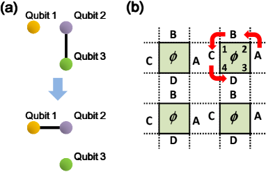
Figure 1: Dynamical creation of chiral interaction. (a) Schematic illustration of generating the chiral interaction $\hat{\chi}_{123}\equiv\vec{\sigma}_{1}\cdot\vec{\sigma}_{2}\times\vec{\sigma}_{3}$ by switching ON/OFF the Heisenberg interactions between qubits. In the first step, the Heisenberg interaction is switched ON between qubits 2 and 3. In the next step, after switching OFF the interaction between qubits 2 and 3, the interaction between qubits 1 and 2 is switched ON. Then, the effective interaction $\hat{\chi}_{123}$ is generated in addition to the Heisenberg couplings. (b),Generating process of the chiral interaction of the form of $(-\hat{\chi}_{123}-\hat{\chi}_{134}-\hat{\chi}_{124}+\hat{\chi}_{234}$) whose expectation value corresponds to Eq. (2), assuming that spin qubits are placed on each node of the square lattice. The interactions between two qubits are switched ON and OFF in the order of A$\rightarrow$B$\rightarrow$C$\rightarrow$D, where A$\sim$D indicate the interactions between two qubits.

Instead of finding materials that have target chiral properties, recent quantum simulation technologies Bloch ; Franco can be applied to dynamically simulate the chirality of a spin system. Here, we propose practical methods of controlling the chirality in a spin-qubit system on a square lattice by switching ON/OFF the interaction between qubits, or initializing the qubit states asymmetrically (spin-up or spin-down). Typical spin-qubits are realized in semiconductor quantum dot (QD) systems Petta ; Koppens ; Maune ; Veldhorst . Each QD includes one excess electron whose spin degree of freedom plays the role of qubit. The exchange coupling $J$ is caused by Coulomb interactions between electrons, and is controlled by the gate electrodes. The switching ON/OFF of the coupling $J$ is more feasible than the control of the arbitrary rotation of each qubit DiVincenzo . In addition, because the coherence time is limited, the quantum operations should be as simple as possible.

In this paper, we provide three methods to create a chiral spin state in a spin-1/2 qubit system on a square lattice by switching ON/OFF of the coupling $J$. As mentioned above, it is difficult to obtain the chiral interaction $\vec{S}_{i}\cdot\vec{S}_{j}\times\vec{S}_{k}$ as the dominant term in the conventional perturbation theory. In the first method, we show that effective chiral Hamiltonians can be designed only by switching ON/OFF the Heisenberg and $XY$ interactions. In the second and third methods, we derive chiral states with arbitrary phase by preparing appropriate initial qubit states. Here, we consider product states of spin-up or spin-down as the initial qubit states. This is because preparation of product states is much easier than that of entangled states. Moreover, focusing on product states makes the discussion simple and clear. In the second method, we show analytical forms of chiral states for four qubits on a square lattice. The third method provides how to control chiralities by preparing appropriate initial qubit states in an always-on lattice system. We show that asymmetrically-arranged qubit states periodically generate the chirality whose phase is $\pi/2$. In this paper, we would like to describe the clear relationship between the phase of the chirality and the asymmetric spin state.

This paper is organized as follows: In Sec. II we show how to generate effective chiral Hamiltonians by switching ON/OFF the coupling between qubits. In Sec. III, we show our second method in which analytical form of the chirality is derived in a four-qubit system. In Sec. IV, we consider the chiral spin state on the always-on lattice system. In Sec. V, we mention experimental possibilities. Sec. VI is devoted to a summary. In Appendix, we show detailed derivations of equations and related numerical calculations.

II Construction of effective chiral Hamiltonian

The chirality is defined around the loop with gauge-invariant form following Ref. WWZ . When $\hat{\chi}_{ij}\equiv\sum_{s=\uparrow\downarrow}\hat{c}_{is}^{\dagger}\hat{c}_{js},$ ($\hat{c}_{is}$ is the electron annihilation operator), the chirality of a square lattice is defined by

$$w_{1234} = \langle\hat{\chi}_{12}\hat{\chi}_{23}\hat{\chi}_{34}\hat{\chi}_{41}\rangle.$$ (1)

In this definition, qubit 1 is the origin and end of the loop. Thus, the asymmetry is discussed from the view of qubit 1. The chiral spin state is defined as a state where the imaginary part of $w_{1234}$ has a finite phase ($w_{1234}=|w_{1234}|\exp i\phi$ and $\phi\neq 0$). The phase $\phi$ of the loop is proportionate to the area of the loop and is important for the topological aspect of the qubit system Rokhsar ; Kitaev ; Ioffe . We treat a spin-1/2 model $\vec{S}_{i}=(1/2)\vec{\sigma}_{i}$, where $\vec{\sigma}_{i}=(\sigma^{x}_{i},\sigma^{y}_{i},\sigma^{z}_{i})$ ($\sigma^{x}_{i}$, $\sigma^{y}_{i}$, and $\sigma^{z}_{i}$ show the Pauli matrices of the lattice site $i$), focusing on the phase of the chirality rather than the properties of the spin-liquid. The expectation value of $E_{123}\equiv\langle\vec{\sigma}_{1}\cdot\vec{\sigma}_{2}\times\vec{\sigma}_{3}\rangle$ has a simple relation with the chirality of the loop WWZ : For the square lattice, we have

$${\rm Im}w_{1234}=\frac{1}{8}(-E_{123}-E_{134}-E_{124}+E_{234}).$$ (2)

Here, the asymmetry of the spin system is introduced by the asymmetric switching of the nearest-neighbor qubit-qubit interaction and the asymmetric spin configuration on the square lattice. First, we show how to obtain the chiral interaction $\vec{\sigma}_{1}\cdot\vec{\sigma}_{2}\times\vec{\sigma}_{3}$ by switching ON/OFF the nearest-neighbor interactions between qubits. For the Heisenberg model, we use the basic relation between three spins given by

$$[\vec{\sigma}_{1}\cdot\vec{\sigma}_{2},\vec{\sigma}_{2}\cdot\vec{\sigma}_{3}]=2i\vec{\sigma}_{2}\cdot\vec{\sigma}_{1}\times\vec{\sigma}_{3}.$$ (3)

The point is that the left commutation relation of this equation is obtained by simply multiplying the time-evolution operators $U_{ij}^{HS}(t)\equiv e^{itH^{HS}_{ij}}=\exp\{iJt\vec{\sigma}_{i}\cdot\vec{\sigma}_{j}\}$ in the Baker-Campbell-Hausdorf formula given by

$$U_{12}^{HS}(t_{1})U_{23}^{HS}(t_{2})=\exp\{iJ(t_{1}\vec{\sigma}_{1}\cdot\vec{\sigma}_{2}+t_{2}\vec{\sigma}_{2}\cdot\vec{\sigma}_{3})$$

$$-J^{2}t_{1}t_{2}/2[\vec{\sigma}_{1}\cdot\vec{\sigma}_{2},\vec{\sigma}_{2}\cdot\vec{\sigma}_{3}]+...\}.$$ (4)

Figure 1(a) shows this process: the first step is switching ON the interaction between spin 2 and 3, and the next step is, after switching OFF this interaction, switching ON the interaction between spin 1 and 2. This process is generalized to obtain the chiral interactions as the next dominant terms of the effective Hamiltonian.

$$H_{\rm eff}=\sum_{ij}J_{ij}\vec{\sigma}_{i}\cdot\vec{\sigma}_{j}+\sum_{ijk}J^{\prime}_{ijk}\vec{\sigma}_{i}\cdot\vec{\sigma}_{j}\times\vec{\sigma}_{k},$$ (5)

where $J^{\prime}_{ijk}=J_{ij}J_{jk}t_{0}.$ under the condition of $J_{ij}t_{0}<1$ when $t_{1}=t_{2}=t_{0}$ in Eq. (4). As an example, the Hamiltonian whose chiral interaction has the form of Eq. (2) is realized by the serial operations given by $U_{34}^{HS}(t)U_{41}^{HS}(t)U_{12}^{HS}(t)U_{23}^{HS}(t)$. Figure 1(b) shows this process graphically.

For the $XY$ Hamiltonian $H^{xy}=\sum_{i<j}H^{xy}_{ij}=\sum_{i<j}J[\sigma_{i}^{x}\sigma_{j}^{x}+\sigma_{i}^{y}\sigma_{j}^{y}]$, we can generate the pure chiral Hamiltonian $H\propto\vec{\sigma}_{1}\cdot\vec{\sigma}_{2}\times\vec{\sigma}_{3}$ by using the equation given by

$$O_{ijk}^{xy}\equiv[U_{jk}^{xy}]^{-1}(\sigma^{x}_{i}\sigma^{x}_{j}+\sigma^{y}_{i}\sigma^{y}_{j})U_{jk}^{xy}=\frac{1}{2}\sigma^{z}_{j}(\sigma^{x}_{k}\sigma^{y}_{i}-\sigma^{x}_{i}\sigma^{y}_{j}).$$

where $U_{ij}^{xy}=\exp i(\pi/4)[\sigma_{i}^{x}\sigma_{j}^{x}+\sigma_{i}^{y}\sigma_{j}^{y}]$. The chiral Hamiltonian $H\propto\vec{\sigma}_{1}\cdot\vec{\sigma}_{2}\times\vec{\sigma}_{3}$ is obtained by the sequence of switching ON/OFF the $XY$ interactions: $O_{123}^{xy}O_{231}^{xy}O_{312}^{xy}$.

III Construction of chiral spin state starting from product states

The above-mentioned method is effective when the target Hamiltonian is not complicated. Here, we provide a simpler method to obtain the chirality directly. When we look at the process of Fig. 1(a), it is found that switching ON one interaction can realize the finite chirality. That is, the expectation value, $w_{1234}^{HS}(t)=\langle\Psi_{0}|U_{23}^{HS\dagger}(t)\hat{\chi}(1234)U_{23}^{HS}(t)|\Psi_{0}\rangle$ with $\hat{\chi}(1234)\equiv\hat{\chi}_{12}\hat{\chi}_{23}\hat{\chi}_{34}\hat{\chi}_{41}$ and $|\Psi_{0}\rangle=|s_{1}s_{2}s_{3}s_{4}\rangle$, is given by $w_{1234}^{HS}(t)=(1+Z_{2}Z_{3})(n_{1\uparrow}n_{4\downarrow}+n_{1\downarrow}n_{4\uparrow})/4-(Z_{2}+Z_{3}+i\sin(4Jt)[Z_{2}-Z_{3}])(n_{1\uparrow}n_{4\downarrow}-n_{1\downarrow}n_{4\uparrow})/4$, where $Z_{i}=\langle s_{i}|\sigma_{i}^{z}|s_{i}\rangle$, and $n_{is}(\in\{0,1\})$ is the number of the $s$-spin for the site $i$ (See the Appendix A and ref tanaSW ; tanaSR ). When $Z_{3}=-Z_{2}$($s_{2}=\uparrow$, $s_{3}=\downarrow$, or $s_{2}=\downarrow$, $s_{3}=\uparrow$), we have $w_{1234}^{HS}(t)=-i\sin(4Jt)Z_{2}(n_{1\uparrow}n_{4\downarrow}-n_{1\downarrow}n_{4\uparrow})/2$. This means that switching ON one interaction itself generates the chirality of a phase $\pi/2$. The same form is obtained for the $XY$ interaction. The chirality of the Ising $XX$ interaction has a similar form except for $\sin(2Jt)$ instead of $\sin(4Jt)$.

Thus, the chiral spin states can be dynamically created by directly manipulating the interactions between qubits. This is because the basic Eq. (3) appears many times in the calculation of the expectation value $w_{1234}$. Moreover, switching ON two interactions enables the generation of the chiral state with a phase in the range of $-\pi$ to $\pi$, as shown in Table I. The case on the left in Table I shows the process shown in Fig. 1(a). The time-saving method is shown in the case on the right in Table I, in which the interaction between 1 and 4 and that between 2 and 3 are simultaneously switched ON (the general expressions are shown in the Appendix). For example, the flux state whose phase is $\pi$ Affleck ; WWZ is given periodically when $4Jt=\pi/2$ for the Heisenberg interaction.

		Chirality of	Chirality of
Ising $XX$		$\{e^{4iJt}-1-2i\sin(2Jt)Z_{1}Z_{2}\}/8$	$e^{-4iJt}(Z_{1}+Z_{2}e^{4iJt})[Z_{2}-Z_{1}]/8$
$XY$		$ie^{2iJt}\sin(4Jt)[Z_{2}-Z_{1}]^{2}/8$	$ie^{-4iJt}\sin(4Jt)[Z_{2}-Z_{1}]^{2}/8$
Heisenberg		$ie^{4iJt}\sin(4Jt)[Z_{2}-Z_{1}]^{2}/8$	$ie^{-4iJt}\sin(4Jt)[Z_{2}-Z_{1}]^{2}/8$

Table I: Switching ON two interactions to create the chiralities with desired phases. The chirality on the square lattice for the three interactions. For simplicity, we show the cases of $Z_{3}=Z_{1}=\langle s_{1}|\sigma_{1}^{z}|s_{1}\rangle$ and $Z_{4}=Z_{2}=\langle s_{2}|\sigma_{2}^{z}|s_{2}\rangle$ ($s_{i}\in\{\uparrow,\downarrow\}$). $Z_{i}=1$ for $s_{i}=\uparrow$ and $Z_{i}=-1$ for $s_{i}=\downarrow$. General form of the left switching pattern, see Appendix  B and C for detail.

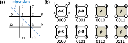
Figure 2: Configuration of spin qubits for the always-on interaction. (a) The twelve qubit sites for numerical calculation of the chirality $w_{1234}$. The sites are connected by the always-on interactions. The dashed line shows the mirror-plane when the chirality is defined by Eq. (1). (b), There are 2${}^{4}=16$ initial states for the spin configurations for the four qubits. Half of the spin configurations of the initial states are illustrated. Other configurations have the same results because of the symmetry. The circle and the double circles indicate the spin-up ($\uparrow$) and the spin-down ($\downarrow$) states, respectively. Colored patterns (0010,0011,0110,0111), whose spin configurations are asymmetric to the mirror-plane of Fig.(a), have a phase $\pi/2$ at $t\sim 0$ (see Fig. 3).

IV Chiral spin state with always-on interactions

Finally, let us consider a case of more restrictive condition in which the interactions between qubits are always-on (Fig. 2(a)). This happens when the distances between qubits are small in order to reduce decoherence. For this case, we generate the chirality only by preparing asymmetric initial qubit states. Because of the commutability of the Ising interactions $[\sigma^{x}_{i}\sigma^{x}_{j},\sigma^{x}_{j}\sigma^{x}_{k}]=0$, the time-dependent chirality of the $XX$ interaction can be derived analytically. On the other hand, the time-dependent chiralities of the $XY$ and the Heisenberg interactions are obtained by numerical calculations.

The chirality of the $XX$ interaction on the square lattice $w_{1234}^{XX}(t)=\langle\Psi_{0}|U^{xx\dagger}(t)\hat{\chi}(1234)U^{xx}(t)|\Psi_{0}\rangle$ with $U^{xx}(t)\equiv\exp\{iJt\sum_{i<j}^{1,..,12}X_{i}X_{j}\}$ and $|\Psi_{0}\rangle=|s_{1}s_{2}s_{3}s_{4}\rangle$ is given by

$$w_{1234}^{XX}(t)\!=\!\!\{\cos^{2}2Jt[Z_{3}(Z_{2}e^{4iJt}+Z_{4}e^{-4iJt})-Z_{2}(Z_{1}-Z_{4})$$ (6)

$$-Z_{1}(Z_{3}+Z_{4})-\cos^{2}2Jt\cdot Z_{1}Z_{2}Z_{3}Z_{4}]+1\}/8.$$

Note that $w_{1234}^{XX}(t)$ is irrelevant to the spin configurations of the qubits around. Thus, when $Z_{2}=-Z_{4}$ (the colored patterns shown in Fig. 2(b)), we have $w_{1234}^{XX}(t)\rightarrow iZ_{3}Z_{2}Jt$ at $t\sim 0$, which means that the chirality of the Ising interaction has a phase $\pi/2$ at $t\sim 0$. Because of the uniform interactions between qubits, the asymmetry is introduced by the asymmetric configuration of the qubit state seen from qubit 1. Figures 3(a) and (b) show the time-dependent amplitude and phase of $w_{1234}^{XX}$ of Eq. (6). Compared with the switching ON one interaction mentioned above, we need to control the four qubit states to obtain the $\pi/2$-phase.

Figures 3(c-f) show the numerically-calculated time-dependent chiralities of the $XY$ and the Heisenberg interactions given by

$$w_{1234}^{XY}(t) = \langle\Psi_{0}|U^{xy\dagger}(t)\hat{\chi}(1234)U^{xy}(t)|\Psi_{0}\rangle,$$ (7)

$$w_{1234}^{HS}(t) = \langle\Psi_{0}|U^{HS\dagger}(t)\hat{\chi}(1234)U^{HS}(t)|\Psi_{0}\rangle,$$ (8)

with $U^{xy}(t)=\exp\{it\sum_{i<j}^{1,..,12}H^{xy}_{ij}\}$, $U^{HS}(t)=\exp\{it\sum_{i<j}^{1,..,12}H^{HS}_{ij}\}$, and $|\Psi_{0}\rangle=|s_{1}s_{2}s_{3}s_{4}\rangle$ including the twelve spin qubits (Fig. 2(a)). The number of qubits included in these calculations comes from the limitation of the calculation resource, and the calculated chiralities of all the states of qubits 5 to 12 in Fig. 2(a) are summed and divided by $2^{8}$. We can see that when $Z_{2}=-Z_{4}$ the chirality has the finite phase. The $\pi/2$ phases around $t\sim 0$ are analyzed by the expansion $w_{1234}(t)\sim\langle\Psi_{0}|\hat{\chi}(1234)+it[\hat{\chi}(1234),H]+O(t^{2})|\Psi_{0}\rangle$, with $H=\sum_{i,j=1}^{12}H_{ij}$ for $H_{ij}=H_{ij}^{HS}$ or $H_{ij}=H_{ij}^{xy}$. Because $\langle\Psi_{0}|\hat{\chi}(1234)|\Psi_{0}\rangle=0$ and $\langle\Psi_{0}|[\hat{\chi}(1234),H]|\Psi_{0}\rangle=(1/2)Z_{3}(Z_{2}-Z_{4})$, $w_{1234}(t)$ has a $\pi/2$ phase around $t\sim 0$. Thus, even in the case of the always-on interaction, the chirality with finite phase can be obtained dynamically for asymmetrical spin configurations.

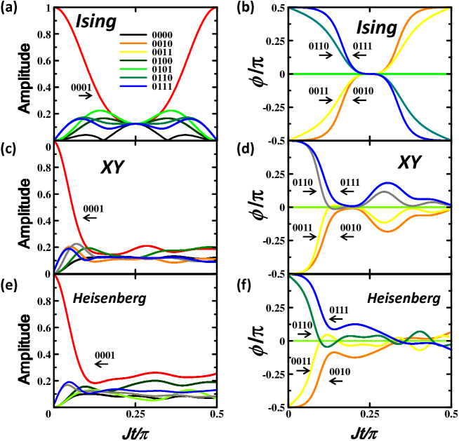
Figure 3: The time-dependent behavior of the chirality $w_{1234}$, Eq. (1), of the square lattice. Always-on interactions are assumed for the configuration of spin-qubits shown in Fig. 2. The left and right figures show the numerical results for the amplitudes $|w_{1234}|$ and the phases $\phi$ of $w_{1234}=|w_{1234}|\exp i\phi$, respectively. (a),(b),The results for the Ising interaction calculated from the analytic form of Eq. (6). (c),(d),The results of the average $w_{1234}$ for the $XY$ interaction numerically calculated from Eq. (7), and (e),(f), the results of the average $w_{1234}$ for the Heisenberg interaction numerically calculated from Eq. (8). For the $XY$ and the Heisenberg interactions, after obtaining $w_{1234}$ for all $2^{12}$ configurations, the average values of $w_{1234}$ are taken over the spin states of the site $5-12$. See Appendix D for details. As seen from (b), the colored patterns (0010,0011,0110,0111) in Fig. 2(b) have a phase $\pi/2$ at $t\sim 0$.

V Discussions

The chiralities calculated here include no relaxation process. In reality, qubit systems couple to the environment and decohere. In the case of GaAs QDs, the coherence is lost mainly through the interaction with the nuclear spins. For $J\approx 0.1$–$1~{}\mu$eV Petta , the coherent change of the chirality is expected to be in the period of $(2J)^{-1}\approx 2.0$–$20$ nsec, which is in the range of the experimental coherence times($<$ 50 ns Koppens ).

As shown in Ref. WWZ , there is a relationship between the expectation value $E_{ijk}$ and the Berry phase ${\cal B}_{ijk}$given by ${\cal B}_{123}-{\cal B}_{132}=(i/2)E_{123}$. Thus, when the Berry phase can be detected as shown in Refs Bertlmann ; Filipp , it might be possible to compare the calculated results here with experiments based on Eq.(2).

In this paper, we considered only product states as the initial states of the qubits. The time-dependent chirality of entangled states is interesting and important. However, because there are many types of entangled states, the chirality of entangled states should be discussed in a separated paper for the sake of clarity. Even if we focus on some specific entangled states, there are still a lot of things to classify the results. As an example, let us consider the chirality of the ground state of the Ising $ZZ$ interaction on a square lattice. The ground state of the four qubits on a square lattice is a degenerated state given by $A|0101\rangle+B|1010\rangle$ with an eigenvalue of $-4J$ ($A$ and $B$ are arbitrary constants). Then the chirality is calculated as $-(A^{*}B+AB^{*})=-\sin(2p)\cos(q)$ when $A=\cos(p)$, $B=\sin(p)\exp(iq)$. Thus, depending on the coefficients $A$ and $B$, the chirality changes variously.

VI Summary

In summary, we have shown simple methods to generate the chiral spin Hamiltonian from conventional spin-spin interactions. We have also shown that, even for the always-on interaction (the conventional spin system), the chiral spin state is realized if the initial state is appropriately prepared.

Appendix A Derivations of chiralities and basic relations

The formulation of the chirality, equation (1), is derived by assuming the half-filled case (one spin per site). The electron annihilation operator $\hat{c}_{is}$ ($s\in\{\uparrow,\downarrow\}$), and the Pauli matrices have the relationship given by

$$\sigma_{i}^{x} = c_{i\uparrow}^{\dagger}c_{i\downarrow}+c_{i\downarrow}^{\dagger}c_{i\uparrow},$$

$$\sigma_{i}^{y} = =-i(c_{i\uparrow}^{\dagger}c_{i\downarrow}-c_{i\downarrow}^{\dagger}c_{i\uparrow}),$$

$$\sigma_{i}^{z} = =c_{i\uparrow}^{\dagger}c_{i\uparrow}-c_{i\downarrow}^{\dagger}c_{i\downarrow},$$

with $\sigma_{i}^{p}\equiv\frac{1}{2}(\sigma^{x}_{i}+i\sigma^{y}_{i})=c_{i\uparrow}^{\dagger}c_{i\downarrow}$, and $\sigma_{i}^{m}\equiv\frac{1}{2}(\sigma^{x}_{i}-i\sigma^{y}_{i})=c_{i\downarrow}^{\dagger}c_{i\uparrow}$.

The explicit form of the chirality $w_{1234}$ given by equation (1) is directly derived by inserting $\hat{\chi}_{ij}\equiv\sum_{s=\uparrow\downarrow}\hat{c}_{is}^{\dagger}\hat{c}_{js}$, and we have,

$$\hat{\chi}_{12}\hat{\chi}_{23}\hat{\chi}_{34}\hat{\chi}_{41} = a_{p}c_{p}+b_{p}d_{m}+a_{m}c_{m}+b_{m}d_{p},$$ (9)

where

$$a_{p} = n_{2\downarrow}n_{3\downarrow}+\sigma_{2}^{m}\sigma_{3}^{p},$$

$$a_{m} = n_{2\uparrow}n_{3\uparrow}+\sigma_{2}^{p}\sigma_{3}^{m},$$

$$b_{p} = -\sigma_{2}^{p}n_{3\downarrow}-n_{2\uparrow}\sigma_{3}^{p},$$

$$b_{m} = -\sigma_{2}^{m}n_{3\uparrow}-n_{2\downarrow}\sigma_{3}^{m},$$

$$c_{p} = n_{1\uparrow}n_{4\downarrow}-\sigma_{1}^{p}\sigma_{4}^{m},$$

$$c_{m} = n_{1\downarrow}n_{4\uparrow}-\sigma_{1}^{m}\sigma_{4}^{p},$$

$$d_{m} = \sigma_{1}^{m}n_{4\downarrow}-n_{1\downarrow}\sigma_{4}^{m},$$

$$d_{p} = \sigma_{1}^{p}n_{4\uparrow}-n_{1\uparrow}\sigma_{4}^{p},$$

with $n_{i\uparrow}=c_{i\uparrow}^{\dagger}c_{i\uparrow}$, and $n_{i\downarrow}=c_{i\downarrow}^{\dagger}c_{i\downarrow}$.

When we derive expectation values accompanying with the unitary transformations $U_{ij}^{HS}(\theta)=\exp\{i\theta\vec{\sigma}_{i}\cdot\vec{\sigma}_{j}\}$, $U_{ij}^{XY}(\theta)=\exp\{i\theta[\sigma_{i}^{x}\sigma_{j}^{x}+\sigma_{i}^{y}\sigma_{j}^{y}]\}$, and $U_{ij}^{XX}(\theta)=\exp\{i\theta\sigma_{i}^{z}\sigma_{j}^{z}\}$, we use the equations given by tanaSW

$$U_{12}^{HS}(-\theta)\sigma^{z}_{1}U_{12}^{HS}(\theta)=\cos^{2}(2\theta)\sigma^{z}_{1}$$

$$+\sin^{2}(2\theta)\sigma^{z}_{2}+\frac{1}{2}\sin(4\theta)(\sigma^{x}_{1}\sigma^{y}_{2}-\sigma^{y}_{1}\sigma^{x}_{2})\>.$$ (10)

and its cyclic relations($x\rightarrow y\rightarrow z\rightarrow x$), for the Heisenberg interaction,

$$\!U_{12}^{XY}(-\theta)\sigma^{x}_{1}U_{12}^{XY}(\theta)\!\!\! \!=\! \!\!\cos(2\theta)\sigma^{x}_{1}-\sin(2\theta)\sigma^{z}_{1}\sigma^{y}_{2},$$ (11)

$$\!U_{12}^{XY}(-\theta)\sigma^{y}_{1}U_{12}^{XY}(\theta)\!\!\! \!=\! \!\!\cos(2\theta)\sigma^{y}_{1}+\sin(2\theta)\sigma^{z}_{1}\sigma^{x}_{2},$$ (12)

$$\!U_{12}^{XY}(-\theta)\sigma^{z}_{1}U_{12}^{XY}(\theta)\!\!\! \!=\! \!\!\cos^{2}(2\theta)\sigma^{z}_{1}+\sin^{2}(2\theta)\sigma^{z}_{2}$$ (13)

$$\!+\! \!\!\frac{1}{2}\sin(4\theta)[\sigma^{x}_{1}\sigma^{y}_{2}-\sigma^{y}_{1}\sigma^{x}_{2}]\>,$$

for $XY$ interaction, and

$$U_{12}^{XX}(-\theta)\sigma^{y}_{1}U_{12}^{XX}(\theta)\!=\!\cos(2\theta)\sigma^{y}_{1}+\sin(2\theta)\sigma^{z}_{1}\sigma^{x}_{2},$$ (14)

$$U_{12}^{XX}(-\theta)\sigma^{z}_{1}U_{12}^{XX}(\theta)\!=\!\cos(2\theta)\sigma^{z}_{1}-\sin(2\theta)\sigma^{y}_{1}\sigma^{x}_{2}\>,$$ (15)

for Ising interaction. The expectation values $\langle\Psi_{0}|\hat{\chi}_{12}\hat{\chi}_{23}\hat{\chi}_{34}\hat{\chi}_{41}|\Psi_{0}\rangle$ are estimated by the product states $|\Psi_{0}\rangle=|s_{1}s_{2}s_{3}s_{4}\rangle$ ($s_{i}\in\{\uparrow,\downarrow\}$).

Appendix B General form of the left method of Table I

The general form for the Heisenberg interaction is given by

$$w_{1234}^{HS} = \frac{1}{8}\left\{1-Z_{1}Z_{2}Z_{3}Z_{4}+Z_{4}Z_{B}-Z_{1}Z_{A}\right.$$ (16)

$$+ \left.e^{4iJt}(Z_{2}Z_{3}-Z_{1}[Z_{B}+Z_{4}]+Z_{4}Z_{A}\right.$$

$$+ \left.i\sin(4Jt)[Z_{4}-Z_{1}][Z_{2}-Z_{3}])\right\},$$

where $Z_{A}=\cos^{2}(2Jt)Z_{2}+\sin^{2}(2Jt)Z_{3}$ and $Z_{B}=\sin^{2}(2Jt)Z_{2}+\cos^{2}(2Jt)Z_{3}$. For the $XY$ interaction, we have

$$w_{1234}^{XY} = \frac{1}{8}\{1-Z_{1}Z_{2}Z_{3}Z_{4}+Z_{4}Z_{B}-Z_{1}Z_{A}$$ (17)

$$+ e^{4iJt}(Z_{2}Z_{3}-Z_{1}[Z_{B}+Z_{4}]+Z_{4}Z_{A})$$

$$+ ie^{2iJt}\sin(4Jt)[Z_{4}-Z_{1}][Z_{2}-Z_{3}])\},$$

For the Ising $XX$ interaction, we have

$$w_{1234}^{XX} = \frac{1}{8}\{(1-e^{2iJt}Z_{1}Z_{2})(1+e^{-2iJt}Z_{3}Z_{4})$$ (18)

$$+ (-Z_{1}+e^{2iJt}Z_{2})(Z_{3}+e^{2iJt}Z_{4})\}.$$

Appendix C General form of the right method of Table I

The general expression of the chirality of the right method of Table I is given by $w_{1234}^{XX}=G_{23}^{-}(\theta)H_{14}^{+}(\theta)+G_{23}^{+}(\theta)H_{14}^{-}(\theta)$ for the Ising $XX$ interaction, and the $XY$ and Heisenberg cases provide the same form of $w_{1234}^{XY}=w_{1234}^{hs}=F_{23}^{-}(\theta)H_{14}^{+}(2\theta)+F_{23}^{+}(\theta)H_{14}^{-}(2\theta)$. where

$$F_{ij}^{\pm}(\theta) \equiv ([1\pm Z_{i}][1\pm Z_{j}]\pm i\sin{4\theta}[Z_{i}-Z_{j}])/4,$$ (19)

$$G_{ij}^{\pm}(\theta) \equiv (1\pm Z_{i}e^{2i\theta})(1\pm Z_{j}e^{-2i\theta})/4,$$ (20)

$$H_{ij}^{\pm}(\theta) \equiv (1-Z_{i}Z_{j}\pm e^{-2i\theta}[Z_{i}-Z_{j}])/4,$$ (21)

Thus, in order to obtain a finite phase, $Z_{4}=-Z_{1}$ or $Z_{3}=-Z_{2}$ are necessary. Table I shows the results for the simple case of $Z_{4}=-Z_{3}=Z_{2}=-Z_{1}$.

Appendix D Numerical calculations

In Fig.3c-f, we have directly calculated equation (1) for the $XY$ and the Heisenberg interactions, as expressed by Eq.(7) and (8), respectively. There are $2^{12}$ patterns of the spin configurations in Fig. 2a. Depending on the spin configuration over the twelve sites of Fig.2a, the time-dependent chirality changes in various ways. Fig. 4 shows a sample of the results of the Heisenberg interaction of the pattern 0010 of Fig.2b. ‘2,18,34,50,66,82’ correspond to the spin configurations of the 12 sites. The spin configuration can be expressed by a binary form of ‘$i_{12}i_{11}i_{10}i_{9}~{}i_{8}i_{7}i_{6}i_{5}~{}i_{4}i_{3}i_{2}i_{1}$’, such that $i_{j}=0$ or 1 ($j=1,...,12$) depending on spin-up or spin-down, respectively. Then the binary form can be transformed to the decimal number given by $i_{12}\cdot 2^{12}+i_{11}\cdot 2^{11}+i_{10}\cdot 2^{10}+i_{9}\cdot 2^{9}+i_{8}\cdot 2^{8}+i_{7}\cdot 2^{7}+i_{6}\cdot 2^{6}+i_{5}\cdot 2^{5}+i_{4}\cdot 2^{4}+i_{3}\cdot 2^{3}+i_{2}\cdot 2^{2}+i_{1}$. For example, ‘2’ corresponds to ’0000 0000 0010’, which means that the spin of site 2 is flipped, and ’18’ corresponds to 0000 0001 0010, which means that the spins of sites 2 and 5 are flipped. It is seen that the phase of the chirality around $t\sim 0$ is $\pi/2$ for all configurations. The time-dependent behaviors for $t>0$ are different depending on their configuration. The results shown in Fig. 3 are the averaged results over all the configurations.

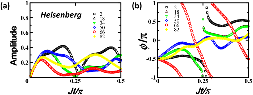
Figure A1: Examples of the calculation of the time-dependent chirality for the Heisenberg Hamiltonian of the twelve qubits before averaging. The ‘2’, ‘18’, ‘34’, ‘50’, ‘66’, and ‘82’ express the qubit states over the twelve sites when 0=$\uparrow$ and 1=$\downarrow$ such as $2=0000~{}0000~{}0010$, $18=0000~{}0001~{}0010$, $34=0000~{}0010~{}0010$, $50=0000~{}0011~{}0010$, $66=0000~{}0100~{}0010$, and $82=0000~{}0101~{}0010$. The last four digits ‘0010’ corresponds to the configuration of the pattern ‘0010’ of Fig. 2b. Other states in the $2^{8}$ configurations show similar behaviors. Fig. 3(e)(f) show the average of these results.

References

(1)
G. L. J. A. Rikken, and E. Raupach,
Nature 390, 493 (1997).
(2)
N. Nagaosa, and Y. Tokura,
Nature Nanotech. 8, 899 (2013).
(3)
Y. Tokunaga, X.Z. Yu, J.S. White, H.M. Rønnow, D. Morikawa, Y. Taguchi, and Y. Tokura,
Nature Comm. 6, 7638 (2015).
(4)
K.S. Ryu, L. Thomas, S.H. Yang, and S. Parkin, Nature Nanotech. 8, 527 (2013).
(5)
S. Emori, U. Bauer, S.M. Ahn, E. Martinez, and G.S.D. Beach, Nature Mater. 12, 611 (2013).
(6)
X. G. Wen,Quantum Field Theory of Many-body Systems.
(Oxford University Press, New York, 2004).
(7)
F. Wilczek, Fractional Statistics and Anyon Superconductivity.
(World Scientific, Singapore, 1990).
(8)
X.G. Wen, F. Wilczek, and A. Zee,
Phys. Rev. B 39, 11413 (1989).
(9)
I. Affleck, and J.B. Marston,
Phys. Rev. B 37, 3774 (1988).
(10)
H. Karapetyan, J. Xia, M. Hucker, G.D. Gu, J.M. Tranquada, M.M. Fejer, and A. Kapitulnik,
Phys. Rev. Lett. 112, 047003 (2014).
(11)
H. Yao, and S.A. Kivelson,
Phys. Rev. Lett. 99, 247203 (2007).
(12)
N.Y. Yao, C.R. Laumann, A.V. Gorshkov, H. Weimer,
L. Jiang, J.I. Cirac, P. Zoller, and M.D. Lukin,
Nature Comms 4, 1585 (2013).
(13)
D. Sen, and R. Chitra,
Phys. Rev. B 51, 1922 (1995).
(14)
Z.Y. Meng, T.C. Lang, S. Wessel, F.F. Assaad, and A. Muramatsu,
Nature 464, 847 (2010).
(15)
O.I. Motrunich,
Phys. Rev. B 73, 155115 (2006).
(16)
D.F. Schroeter, E. Kapit, R. Thomale, and M. Greiter,
Phys. Rev. Lett. 99, 097202 (2007).
(17)
I. Bloch, J. Dalibard, and S. Nascimbène, Nature Phys. 8, 267 (2012).
(18)
I.M. Georgescu, S. Ashhab, and F. Nori,
Rev. Mod. Phys. 86, 153 (2014).
(19)
J.R. Petta, A.C. Johnson, J.M. Taylor, E.A. Laird, A. Yacoby,
M.D. Lukin, C.M. Marcus, M.P. Hanson, and A.C. Gossard,
Science 309, 2180 (2005).
(20)
F.H.L. Koppens, K.C. Nowack, and L.M.K. Vandersypen,
Phys. Rev. Lett. 100, 236802 (2008)
(21)
B.M. Maune, A.E. Schmitz, M. Sokolich, C.A. Watson, M.F. Gyure, and A.T. Hunter,
Nature 481, 344 (2012).
(22)
M. Veldhorst, C.H. Yang, J.C.C. Hwang, W. Huang, J.P. Dehollain, J.T. Muhonen, S. Simmons,
A. Laucht, F.E. Hudson, K.M. Itoh, A. Morello, and A.S. Dzurak,
Nature 526, 410(2015).
(23)
D.P. DiVincenzo, D. Bacon, J. Kempe, G. Burkard, and K.B. Whaley,
Nature 408, 339-342 (2000).
(24)
A. Kitaev,
Annals of Physics 321, 2 (2006).
(25)
L.B. Ioffe, M.V. Feigel’man, A. Ioselevich,
D. Ivanov, M. Troyer, and G. Blatter,
Nature 415, 503(2002).
(26)
D.S. Rokhsar, Phys. Rev. Lett. 65, 1506 (1990).
(27)
T. Tanamoto,
Phys. Rev. A. 88, 062334 (2013).
(28)
T. Tanamoto, K. Ono, Y.X. Liu, and F. Nori,
Scientific Rep. 5, 10076 (2015).
(29)
R. A. Bertlmann, K. Durstberger, Y. Hasegawa, and B. C. Hiesmayr,
Phys. Rev. A 69, 032112 (2004).
(30)
S. Filipp, J. Klepp, Y. Hasegawa, C. Plonka-Spehr, U. Schmidt, P. Geltenbort, and H. Rauch,
Phys. Rev. Lett. 102, 030404 (2009).