Resistivity Minimum in Highly Frustrated Itinerant Magnets

Abstract

We study the transport properties of frustrated itinerant magnets comprising localized classical moments, which interact via exchange with the conduction electrons. Strong frustration stabilizes a liquidlike spin state, which extends down to temperatures well below the effective Ruderman-Kittel-Kasuya-Yosida interaction scale. The crossover into this state is characterized by spin structure factor enhancement at wave vectors smaller than twice the Fermi wave vector magnitude. The corresponding enhancement of electron scattering generates a resistivity upturn at decreasing temperatures.

Certain magnetic metals exhibit a resistivity minimum at low temperature. The Kondo effect explains this minimum via an effective exchange interaction $J$ between magnetic impurities and conduction electrons Kondo (1964). Resistivity minima are also observed in compounds comprising a periodic array of localized magnetic moments such as $4f$-electron compounds Hewson (1993). Because the Kondo effect is induced by spin-flip impurity scattering, it is expected to be strongly suppressed in systems with large local magnetic moments or with strong easy-axis spin anisotropy. Surprisingly, several compounds in this category, such as Gd₂PdSi₃ and $R$CuAs₂ ($R$=Sm, Gd, Tb, and Dy) Mallik et al. (1998); Sampathkumaran et al. (2003); Sengupta et al. (2004) and $R$InCu₄ ($R$=Gd, Dy, Ho, Er, and Tm) Fritsch et al. (2005, 2006), exhibit a pronounced resistivity minimum despite heavy suppression of the Kondo effect. These compounds are dominated by the Ruderman-Kittel-Kasuya-Yosida (RKKY) interaction, which competes against Kondo screening. It is natural to ask, therefore, if there exists a general mechanism by which a RKKY interaction can induce a resistivity minimum AA .

In this Letter, we answer the question affirmatively: frustrated itinerant magnets can exhibit a low-$T$ liquidlike spin state with enhanced resistivity under quite general conditions. For simplicity, we focus on a 2D Kondo lattice model (KLM) with classical local moments (no Kondo effect) and a small Fermi surface (FS). For a circular FS, the bare magnetic susceptibility $\chi^{0}_{\bm{k}}$ of the conduction electrons has a flat area of maxima for $k\leq 2k_{F}$ (where $k\equiv|\bm{k}|$ and $k_{F}$ is the magnitude of Fermi wave vectors). The RKKY interaction thus seeks to enhance the structure factor (SF) in the region $k\leq 2k_{F}$. We demonstrate that this effect leads to an increase of the electrical resistivity $\rho$ upon decreasing the temperature over the window $T_{0}\lesssim T\lesssim|\theta_{\rm CW}|$, where the magnetic correlation length increases from one lattice space $a$ (at $|\theta_{\rm CW}|$) to $\xi\gg a$ (at $T_{0}$) . Frustration ($|\theta_{\rm CW}|/T_{0}\gg 1$) is required just to open this window; the rest is done by the nature of the RKKY interaction. The average enhancement of the spin SF for wave vectors connecting points on the FS increases the elastic electron-spin scattering upon lowering $T$.

The effect of the RKKY interaction on electron transport was considered in Refs. Liu et al. (1987) and Ruvalds and Sheng (1988). The sign of the effect was found to be opposite (metallic) to that found in this Letter. This difference arises because we consider low filling, where the sign of $d\rho/dT$ can be shown to be insulating under quite general assumptions about the SF. In contrast, Refs. Liu et al. (1987) and Ruvalds and Sheng (1988) considered a large FS, where the effect can have either sign depending on details of the electronic structure.

We first present an analytical derivation of the effect for the weak-coupling (WC) limit [$J\eta(\varepsilon_{F})\ll 1$, where $\eta(\varepsilon_{F})$ is the density of states at the Fermi level]. The resistivity is evaluated in the Born approximation and the spin SF is obtained in two ways: from a high-$T$ expansion Oitmaa et al. (2006) and by using the spherical approximation Stanley (1968); Conlon and Chalker (2010). Finally, we perform large-scale simulations of the full KLM. We use a variant of the kernel polynomial method (KPM) Weiße et al. (2006); Barros and Kato (2013); Barros et al. (2014) to integrate Langevin dynamics (LD) and to evaluate the resistivity using the Kubo formula Kubo (1957). Our KPM-LD simulations on a triangular lattice (TL) with $256^{2}$ sites confirm the WC results and generalize them to the intermediate and strong-coupling regimes.

We consider the KLM,

$${\cal H}\!=\!\!\sum_{\bm{k},\sigma}(\varepsilon_{\bm{k}}-\mu)c_{\bm{k}\sigma}^{\dagger}c_{\bm{k}\sigma}^{\;}\!+\!\frac{J}{\sqrt{N}}\!\!\sum_{{\bm{q}},{\bm{k}},\sigma,\sigma^{\prime}}\!\!\!\!\!c_{{\bm{q}}\sigma}^{\dagger}{\bm{\sigma}}_{\sigma\sigma^{\prime}}c_{{\bm{q}}+{\bm{k}}\sigma^{\prime}}^{\;}\!\cdot\!{\bm{S}}_{\bm{k}}.$$ (1)

The operator $c_{{\bm{k}}\sigma}^{\dagger}(c_{{\bm{k}}\sigma}^{\;})$ creates (annihilates) an itinerant electron with momentum ${\bm{k}}$ and spin $\sigma$. $\varepsilon_{\bm{k}}=-\sum_{\bm{\delta}}t_{\bm{\delta}}e^{i{\bm{k}}\cdot{\bm{\delta}}}$ is the bare electronic dispersion relation with chemical potential $\mu$ and hopping amplitudes $t_{\bm{\delta}}$ between sites connected by ${\bm{\delta}}$. The second term is the exchange interaction between the conduction electrons and the local magnetic moments ${\bm{S}}_{\bm{k}}$ in Fourier space. We assume classical moments with magnitude $|\bm{S}_{i}|=1$ ($\bm{\sigma}$ is the vector of the Pauli matrices).

The conduction electrons can be integrated out in the WC limit by expanding in the small parameter $J\eta(\varepsilon_{F})$. The resulting RKKY spin Hamiltonian is

$$H_{\mathrm{RKKY}}=-J^{2}\sum_{\bm{k}}\chi^{0}_{\bm{k}}{\bm{S}}_{\bm{k}}\cdot{\bm{S}}_{\bar{\bm{k}}}$$ (2)

with ${\bar{\bm{k}}}\equiv-{\bm{k}}$ and ${\bm{S}}_{\bm{k}}=\sum_{l}e^{i{\bm{k}}\cdot{\bm{r}}_{l}}{\bm{S}}_{l}/\sqrt{N}$ ($N$ is the total number of lattice sites). The effective coupling constant in momentum space is $-J^{2}\chi^{0}_{\bm{k}}$ with $\chi^{0}_{\bm{k}}=T\sum_{\bm{q},\omega_{n}}G^{0}_{\bm{q},\omega_{n}}G^{0}_{\bm{q}+\bm{k},\omega_{n}}$, where $\omega_{n}=(2n+1)\pi T$ are the Matsubara frequencies and $G^{0}_{\bm{k},\omega_{n}}=\left\{i\omega_{n}-\left[\varepsilon_{\bm{k}}-\mu\right]\right\}^{-1}$ is the bare Green’s function. Then, the RKKY interaction favors magnetic orderings that maximize $\chi^{0}_{\bm{k}}$.

The electrons feel an effective potential produced by the spin configuration through the exchange interaction $J$. If the system orders at low-enough temperature $(T\leq T_{c})$, the periodic array of spins only produces coherent electron scattering, which does not contribute to $\rho$ . However, the situation changes above $T_{c}$ because the magnetic moments develop liquidlike correlations, which produce incoherent elastic electron-spin scattering. Within the Born approximation, the scattering cross section is proportional to the spin SF,

$${\cal S}({\bm{k}})=\frac{1}{N}\sum_{jl}e^{i{\bm{k}}\cdot({\bm{r}}_{j}-{\bm{r}}_{l})}\langle{\bm{S}}_{j}\cdot{\bm{S}}_{l}\rangle=\langle{\bm{S}}_{\bm{k}}\cdot{\bm{S}}_{\bar{\bm{k}}}\rangle,$$ (3)

where $\langle\cdots\rangle$ denotes the thermodynamic average. ${\cal S}({\bm{k}})$ satisfies the sum rule $\sum_{\bm{k}}{\cal S}({\bm{k}})=N$ because $|\bm{S}_{i}|=1$. Unlike the high-$T$ gas regime, characterized by a nearly ${\bm{k}}$-independent spin SF, short-range magnetic correlations appear in the liquid regime. The RKKY interaction is expected to enhance ${\cal S}({\bm{k}})$ for wave vectors connecting points on the FS because those are the processes that more effectively reduce the electronic energy. Given that the same processes contribute to the incoherent elastic scattering in the paramagnetic state, $\rho$ should increase upon reducing $T$ from the high-$T$ gas regime to the $T_{0}\lesssim T\lesssim|\theta_{\rm CW}|\sim J^{2}/t$ liquidlike regime.

To illustrate this point we will consider the simple case of a circular FS, relevant for most 2D lattices with a low electron (hole) filling fraction . The dispersion relation near the bottom (top) of the band can be approximated by $\varepsilon_{\bm{k}}\simeq{\bm{k}}^{2}/2m$. The resulting RKKY Hamiltonian is strongly frustrated: any spiral with wave vector ${\bm{k}}$ is a ground state as long as $k\leq 2k_{F}$. The RKKY interaction favors these magnetic configurations because those are the only spirals that can scatter electrons between points ${\bm{q}}$ and ${\bm{q}}+{\bm{k}}$ on the FS.

Within the Born approximation, the inverse relaxation time for elastic scattering is

$$\frac{1}{\tau_{k_{F}}}=\frac{4\pi J^{2}}{N}\sum_{\bm{k}}\delta(\varepsilon_{F}-\varepsilon_{\bm{k}}){\cal S}({\bm{k}}-{\bm{k}}_{F})(1-\cos{\theta_{{\bm{k}}_{F},{\bm{k}}}}).$$ (4)

This expression is further simplified if ${\cal S}({\bm{k}})={\cal S}(k)$, which is a good approximation for low carrier filling fractions in the integration domain $k<2k_{F}$:

$$\frac{1}{\tau_{k_{F}}}=4\pi mJ^{2}c\int^{1}_{0}dx\frac{x^{2}}{\sqrt{1-x^{2}}}\,{\cal S}(2k_{F}x),$$ (5)

where $c$ is a number that depends on the lattice, e.g., $c=\sqrt{3}/\pi^{2}$ for a TL. The $T$ dependence of $\tau_{k_{F}}$ is then determined by the variation of ${\cal S}(k)$ for $k\leq 2k_{F}$.

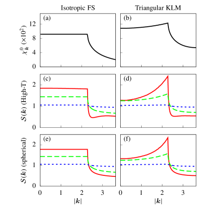
Figure 1: Bare electronic susceptibility for (a) a 2D electron gas with isotropic dispersion $\varepsilon_{\bm{k}}=k^{2}/2m$, and (b) a TL with NN hopping ($t=1$) and filling fraction $n=0.09$. Panels (c)–(f) show the momentum dependence of ${\cal S}({\bm{k}})$ at temperatures $T=\{0.03,0.06,0.45\}J^{2}/t$ represented by solid, dashed, and dotted curves, respectively. Panels (c) and (d) are obtained from a high-$T$ expansion [see Eq. (6)], while panels (e) and (f) are obtained from the spherical approximation. Each panel is calculated using the bare magnetic susceptibility vertically above it. For panels (d) and (f) we assume $\mathcal{S}({\bm{k}})\simeq\mathcal{S}(k)$, which is correct to within 1% relative error.

We will use two independent approaches for computing the $T$ dependence of ${\cal S}(k)$ in the gas and liquidlike regimes. The first approach is a straightforward high-$T$ expansion Oitmaa et al. (2006):

$${\cal S}({\bm{k}}) = 1+K{\tilde{\chi}}_{\bm{k}}+K^{2}\left[{\tilde{\chi}}^{2}_{\bm{k}}-\langle{\tilde{\chi}}^{2}\rangle\right]+K^{3}\big{[}{\tilde{\chi}}^{3}_{\bm{k}}-\langle{\tilde{\chi}}^{3}\rangle$$ (6)

$$-2{\tilde{\chi}}_{\bm{k}}\langle{\tilde{\chi}}^{2}\rangle+\frac{2}{5N^{2}}\sum_{{\bm{q}}{\bm{q}}^{\prime}}{\tilde{\chi}}_{\bm{q}}{\tilde{\chi}}_{\bm{q}^{\prime}}{\tilde{\chi}}_{{\bm{k}}-{\bm{q}}-{\bm{q}^{\prime}}}\big{]}$$

with $K=2J^{2}\beta/3$, ${\tilde{\chi}}_{\bm{k}}={\chi}^{0}_{\bm{k}}-\langle{\chi}\rangle$, and $\langle{\tilde{\chi}}^{n}\rangle=\sum_{\bm{k}}{\tilde{\chi}}^{n}_{\bm{k}}/N$. Figure 1(a) shows the bare magnetic susceptibility for the isotropic FS under consideration. Figure 1(b) shows the bare susceptibility for a TL with nearest-neighbor (NN) hopping $t$ and an electron filling fraction $n=0.09$ (the mass is $m=1/3t$). As expected, the effect of the small $C_{6}$ lattice anisotropy (of order $k^{6}_{F}$) is to split the large global maxima degeneracy that would correspond to an isotropic ${\chi}^{0}_{\bm{k}}$. We will see that this splitting does not alter significantly the window of stability of the liquidlike regime. Figures 1(c) and 1(d) show the momentum dependence of the SF at different temperatures obtained from Eq. (6) for the isotropic FS and the triangular KLM, respectively.

To understand the insulating sign of the temperature dependence of $1/\tau$, it suffices to analyze the second term in Eq. (6), which gives the leading order contribution to the momentum dependence of ${\cal S}({\bm{k}})$. Since $\chi_{k}>0$, the prefactor of the $1/T$ term in $1/\tau$ is positive as long as the average of $\chi_{k}$ over the interval $(0,2k_{F})$ in Eq. (5) exceeds the contribution from $\langle\chi\rangle$, which is just a constant times $\langle\chi\rangle$. Suppose that $\chi^{0}_{k}$ does not vary dramatically in the interval $(0,2k_{F})$, where it can be estimated by some typical value $\bar{\chi}$, and falls off quickly for $k_{F}\ll k\ll b$, where $b\sim 1$ is the reciprocal lattice spacing. Then, the contribution of $\chi_{k}^{0}$ to the integral in Eq. (5) is on the order of $\bar{\chi}$. On the other hand, $\langle\chi\rangle$ is an average value over the entire Brillouin zone, normalized by its area. Therefore, $\langle\chi\rangle\sim\bar{\chi}(k_{F}/b)^{2}$, and the contribution from $\chi_{k}^{0}$ is reduced only by a small correction of order $(k_{F}/b)^{2}$ sup .

Compared with the high-$T$ expansion, the so-called spherical approximation Stanley (1968); Conlon and Chalker (2010) is less well controlled, but can be applied to a wider temperature range. The hard constraints $|{\bm{S}}_{i}|=1$ are replaced with a global soft constraint $\sum_{i}|\bm{S}_{i}|^{2}=N$, which renders the spin Hamiltonian quadratic and can be easily integrated to give ${\cal S}({\bm{k}})=\frac{3T}{2[\Delta(T)-J^{2}{\tilde{\chi}}_{\bm{k}}]}$, where $\Delta(T)$ is determined from the self-consistency equation sup : $\frac{1}{N}\sum_{\bm{k}}J^{2}/[\Delta(T)-J^{2}{\tilde{\chi}}_{\bm{k}}]=K.$ Figures 1(e) and 1(f) show that the results for the isotropic FS and the triangular KLM agree with Figs. 1(c) and 1(d) down to $T\simeq 0.03J^{2}/t$, at which point the high-$T$ expansion fails.

The electrical conductivity is given by

$$\sigma=-\frac{e^{2}}{2}\int\frac{\sqrt{3}d^{2}k}{8\pi^{2}}\tau_{k}v_{k}^{2}\frac{df(\varepsilon_{k})}{d\varepsilon_{k}}\simeq\frac{3\sqrt{3}e^{2}}{8\pi}tk^{2}_{F}\tau_{k_{F}}.$$ (7)

Replacing $\tau_{k_{F}}$ with its expression given in Eq. (5), we obtain

$$\rho(T)=\frac{4}{\pi}\rho_{0}\int^{1}_{0}dx\frac{x^{2}}{\sqrt{1-x^{2}}}{\cal S}(2k_{F}x),$$ (8)

where $\rho_{0}=8\pi J^{2}/(3tek_{F})^{2}$. Figure 2(a) compares the resistivity curves $\rho(T)$ obtained from the high-$T$ expansion and from the spherical approximation. As expected from the comparison of the magnetic SF, the resistivity curves practically coincide down to $T\simeq 0.03J^{2}/t$. Both curves confirm our main conjecture $d\rho/dT<0$ because the system develops stronger spin-spin correlations for wave vectors $k\leq 2k_{F}$. This increase should be interrupted at $T=T_{0}$ where precursors of magnetic Bragg peaks develop from the broad peaks of the liquid state and the Born approximation ceases to be valid.

The analytical approach that we have used for computing $\rho(T)$ is only valid in the WC regime. Away from the WC regime, the RKKY theory is no longer valid as an effective low-energy theory for the KLM and the Born approximation is no longer justified. Moreover, the two different approaches that we used for computing ${\cal S}({\bm{k}})$ fail at low $T$. Our calculations then need to be complemented with numerical simulations valid for any coupling strength and down to arbitrarily low $T$.

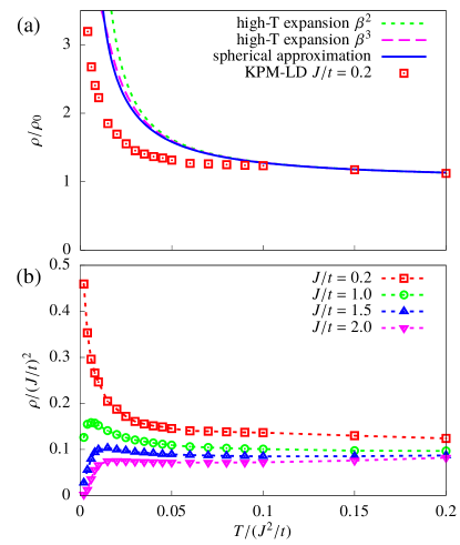
Figure 2: (a) Temperature dependence of the resistivity for a triangular KLM with NN hopping ($t=1$) and filling fraction $n=0.09$. The lines correspond to calculations based on the the Born approximation [see Eq. (8)] and different analytical approaches for computing the temperature dependence of ${\cal S}({\bm{k}})$. The symbols correspond to the results of KPM-LD simulations rescaled by $\rho(T=J^{2}/t)$. (b) Resistivity curve (in units of $h/e^{2}$) obtained from KPM-LD simulations for different coupling strengths com .

We perform KPM-LD simulations on a $256\times 256$ TL with small electron filling $n=0.09$ and $J/t=(0.2,1.0,1.5,2.0)$ . We integrate the dimensionless stochastic Landau-Lifshitz dynamics with a unit damping parameter using the Heun-projected scheme Mentink et al. (2010) for a total of $(2\times 10^{3},4\times 10^{3},6\times 10^{3},1\times 10^{4})$ time steps of duration $\Delta\tau=(100,10,5,2)$. We estimate the effective spin forces using the gradient transformation described in Ref. Barros and Kato, 2013. To decrease the stochastic error, we use the probing method of Ref. Tang and Saad, 2012 with $R=128$ random vectors. The Chebyshev polynomial expansion order is $M=500$. To calculate the resistivity, we expand the Kubo-Bastin formula Kubo (1957); Bastin et al. (1971) using the KPM Weiße et al. (2006); García et al. (2015) with $M=(6000,1000,1000,500)$ . For each temperature, we average the longitudinal conductivity over ten snapshots separated by $(100,100,200,500)$ integration time steps.

Figure 2(b) shows the numerical $\rho(T)$ results for the different $J/t$ values. Frustration decreases with $J/t$ because higher order contributions (beyond RKKY level) split the degeneracy for $k\leq 2k_{F}$. For the strong-coupling limit $J\gg t$ the low-energy sector of ${\cal H}$ can be mapped into a double-exchange model, which favors ferromagnetic (FM) ordering at a critical temperature $T_{c}$ comparable to $|\theta_{\rm CW}|$. Given that the temperature window with liquidlike correlations diminishes as a function of $J/t$, the relative low-temperature upturn of $\rho(T)$ should also decrease, as shown in Fig. 2(b).

In the intermediate-coupling regime $J/t=1$, 1.5, and 2, the low-$T$ upturn of $\rho(T)$ reaches a maximum at temperature $T_{0}$ and drops rapidly for $T<T_{0}$. This crossover corresponds to the enhanced SF at wave vectors $k<2k_{F}$. Figures 3(a) and 3(b) show the temperature dependence of ${\cal S}({\bm{k}})$ for $J/t=1$ and $2$, respectively. The roughly uniform weight of ${\cal S}({\bm{k}})$ for $k<2k_{F}$ starts redistributing below $T\approx 0.006J^{2}/t$. When $J/t\approx 1$ we observe the formation of a ring in Fourier space at $T\approx T_{0}$. This disordered phase is dynamically trapped at the lowest temperatures, $T\lesssim 0.002J^{2}/t$. As expected from the strong-coupling analysis, its radius $k_{0}<2k_{F}$ decreases with $J/t$. For larger couplings $J/t\gtrsim 2$ the FM phase clearly wins at low $T$. We note that, for $T>T_{0}$, there is strong backward scattering produced by the $k\lesssim 2k_{F}$ components of ${\cal S}({\bm{k}})$. The resistivity drops below $T_{0}$ because the backscattering contribution ($k=2k_{F}$) is reduced by the formation of a ring at $k_{0}<2k_{F}$ [see the integrand of Eq. (8)].

Here, we have only considered the resistivity component arising from electron-spin scattering. Electron-electron and electron-phonon scattering also contribute to $\rho$ in real materials. These additional contributions increase with $T$, whereas we have argued that the electron-spin scattering produces a negative $d\rho/dT$. The combination thus yields a resistivity minimum . Although we have assumed classical local spins ($S\rightarrow\infty$), our results can be extended to arbitrary $S$. The generalization of Eq. (6) is straightforward . The main qualitative change is the Kondo effect expected for quantum spins and the antiferromagnetic exchange $J$. This effect becomes apparent by applying the $T$-matrix formalism up to order $J^{3}$ to the KLM sup , which yields

$$\rho(T)\approx\rho_{\text{RKKY}}(T)\left[1-8J\eta(\epsilon_{F})\ln\left(\frac{k_{B}T}{D}\right)\right],$$ (9)

where $\rho_{\text{RKKY}}(T)$ is given in Eq. (8). $\rho_{\text{RKKY}}(T)$ becomes $T$ independent at $T\gg|\theta_{\rm CW}|$, so the only $T$ dependence arises from the Kondo effect. According to Eq. (9), the Kondo logarithmic behavior crosses over into a power law sup

$$\rho_{\text{RKKY}}(T)\sim\frac{a}{T-T^{*}}+b,$$ (10)

upon entering the range $T_{0}\lesssim T\lesssim|\theta_{\rm CW}|$. The qualitatively different $T$ dependence should allow us to distinguish between the two mechanisms for the resistivity upturn. Moreover, the upturn produced by the RKKY mechanism should be accompanied by a corresponding upturn in the correlation length $\xi$. Indeed, moderately frustrated materials, such as Gd₂PdSi₃ and $R$CuAs₂ ($R$=Sm, Gd, Tb, and Dy) Mallik et al. (1998); Sampathkumaran et al. (2003); Sengupta et al. (2004), exhibit a nonlogarithmic resistivity upturn right above the Néel temperature. According to Refs. Udagawa et al. (2012); Chern et al. (2013), the resistivity minimum of the pyrochlore oxides Pr₂Ir₂O₇ and Nd₂Ir₂O₇ is also caused by spin-spin correlations described by the spin ice model.

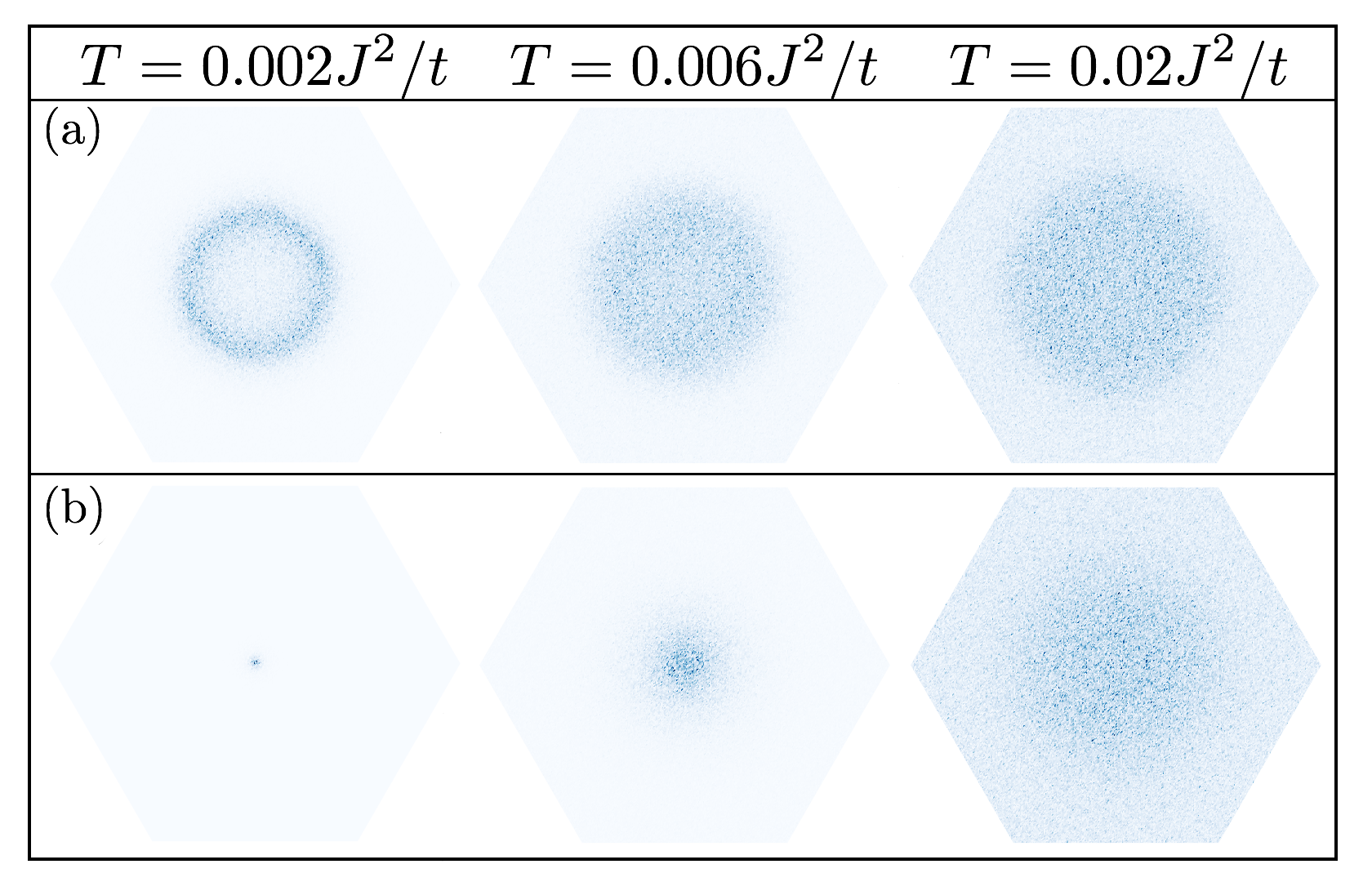
Figure 3: Structure factor ${\cal S}({\bm{k}})$ for three temperatures at intermediate couplings (a) $J/t=1$ and (b) $J/t=2$. At $T\approx 0.02J^{2}/t$, ${\cal S}({\bm{k}})$ is nearly uniformly distributed in the disk $k\lesssim 2k_{F}$. Around $T\approx 0.006J^{2}/t$ the weight begins shifting toward a $k\lesssim 2k_{F}$ radius ring ($J/t\approx 1$) or $k=0$ FM order ($J/t\gtrsim 2$).

Furthermore, the Kondo effect is absent in transition metal oxides, where $J$ is FM (Hund’s coupling). Our results indicate that the resistivity upturn persists in the intermediate coupling regime, relevant to these materials. Indeed, a resistivity upturn has been observed in (Ga_1-xMn_x)As Matsukura et al. (1998); Jungwirth et al. (2006) and manganites Salamon and Jaime (2001) above the FM transition temperature $T_{c}$.

Our key conclusion is that the RKKY interaction enhances the elastic electron-spin scattering by increasing the magnetic SF for wave vectors connecting points on the FS. Assuming that this enhancement eventually leads to Bragg peaks (for $T<T_{c}$), which do not produce incoherent scattering, frustration is necessary to open a wide enough temperature window (liquidlike regime) over which the resistivity upturn becomes noticeable. Although we have focused on 2D systems with a small FS, the conclusion applies generally to frustrated itinerant magnets, provided that $\chi^{0}_{\bm{k}}$ is larger on average for wave vectors $\bm{k}$ connecting points on the FS.

—Supplemental Material—

I Perturbation Theory for KLM

For a Kondo lattice model (KLM), the temperature dependence of the resistivity has contributions from single spin-flip scattering (Kondo effect), and from multi-spin scattering processes, which are controlled by the RKKY mechanism discussed in this paper. Below, we show how both effects contribute to the transport to lowest non-trivial order in perturbation theory.

We consider the KLM in the main text $\mathcal{H}=\mathcal{H}_{0}+\mathcal{H}_{1}$, and allow the local moments to be quantum mechanical spins:

$$\mathcal{H}_{0} =\sum_{\bm{k},\sigma}(\varepsilon_{\bm{k}}-\mu)c_{\bm{k}\sigma}^{\dagger}c_{\bm{k}\sigma}^{\;},$$ (S1a)

$$\mathcal{H}_{1} =\frac{J}{\sqrt{N}}\sum_{{\bm{q}},{\bm{k}},\sigma,\sigma^{\prime}}c_{{\bm{q}}\sigma}^{\dagger}{\bm{\sigma}}_{\sigma\sigma^{\prime}}c_{{\bm{q}}+{\bm{k}}\sigma^{\prime}}^{\;}\cdot{\bm{S}}_{\bm{k}}.$$ (S1b)

The inverse relaxation time is obtained from the T-matrix formalism:

$$\frac{1}{\tau_{\bm{q}}}=2\pi\sum_{\bm{k}}\delta(\epsilon_{\bm{q}}-\epsilon_{\bm{k}})\sum_{\sigma\sigma^{\prime}}\left|T_{\bm{q}\sigma,\bm{k}\sigma^{\prime}}\right|^{2}\left(1-\cos\theta_{\bm{q},\bm{k}}\right),$$ (S2)

where the T-matrix is

$$T=\mathcal{H}_{1}+\mathcal{H}_{1}G_{0}\mathcal{H}_{1},$$ (S3)

up to second order in $J$ and $G_{0}$ is the non-interacting electronic Green’s function. More explicitly:

$$T_{\bm{q}\uparrow,\bm{k}\uparrow} =\frac{J}{\sqrt{N}}S_{\bm{k}-\bm{q}}^{z}+\frac{J^{2}}{N}\sum_{\bm{p}}\Bigg{[}-\frac{2}{\sqrt{N}}S_{\bm{k}-\bm{q}}^{z}\frac{1-f(\epsilon_{\bm{p}})}{\epsilon_{\bm{k}}-\epsilon_{\bm{p}}}$$

$$\quad+\frac{S_{\bm{p}-\bm{q}}^{z}S_{\bm{k}-\bm{p}}^{z}+S_{\bm{k}-\bm{p}}^{+}S_{\bm{p}-\bm{q}}^{-}}{\epsilon_{\bm{k}}-\epsilon_{\bm{p}}}\Bigg{]},$$ (S4a)

$$T_{\bm{q}\downarrow,\bm{k}\downarrow} =-\frac{J}{\sqrt{N}}S_{\bm{k}-\bm{q}}^{z}+\frac{J^{2}}{N}\sum_{\bm{p}}\Bigg{[}-\frac{2}{\sqrt{N}}S_{\bm{k}-\bm{q}}^{z}\frac{f(\epsilon_{\bm{p}})}{\epsilon_{\bm{k}}-\epsilon_{\bm{p}}}$$

$$\quad+\frac{S_{\bm{p}-\bm{q}}^{z}S_{\bm{k}-\bm{p}}^{z}+S_{\bm{p}-\bm{q}}^{+}S_{\bm{k}-\bm{p}}^{-}}{\epsilon_{\bm{k}}-\epsilon_{\bm{p}}}\Bigg{]},$$ (S4b)

$$T_{\bm{q}\downarrow,\bm{k}\uparrow} =\frac{J}{\sqrt{N}}S_{\bm{k}-\bm{q}}^{+}+\frac{J^{2}}{N}\sum_{\bm{p}}\Bigg{[}\frac{1}{\sqrt{N}}S_{\bm{k}-\bm{q}}^{+}\frac{2f(\epsilon_{\bm{p}})-1}{\epsilon_{\bm{k}}-\epsilon_{\bm{p}}}$$

$$\quad+\frac{S_{\bm{p}-\bm{q}}^{+}S_{\bm{k}-\bm{p}}^{z}-S_{\bm{k}-\bm{p}}^{+}S_{\bm{p}-\bm{q}}^{z}}{\epsilon_{\bm{k}}-\epsilon_{\bm{p}}}\Bigg{]},$$ (S4c)

$$T_{\bm{q}\uparrow,\bm{k}\downarrow} =\frac{J}{\sqrt{N}}S_{\bm{k}-\bm{q}}^{-}+\frac{J^{2}}{N}\sum_{\bm{p}}\Bigg{[}\frac{1}{\sqrt{N}}S_{\bm{k}-\bm{q}}^{-}\frac{2f(\epsilon_{\bm{p}})-1}{\epsilon_{\bm{k}}-\epsilon_{\bm{p}}}$$

$$\quad+\frac{S_{\bm{k}-\bm{p}}^{-}S_{\bm{p}-\bm{q}}^{z}-S_{\bm{p}-\bm{q}}^{-}S_{\bm{k}-\bm{p}}^{z}}{\epsilon_{\bm{k}}-\epsilon_{\bm{p}}}\Bigg{]},$$ (S4d)

where $f(\epsilon)$ is the Fermi distribution function.

For elastic scattering in the paramagnetic phase, it follows that

$$\sum_{\sigma\sigma^{\prime}}\!\left|T_{\bm{q}\sigma,\bm{k}\sigma^{\prime}}\right|^{2}\!\!=\!\!\frac{2J^{2}}{N}\mathcal{S}(\bm{k}-\bm{q})\!\!\left[1\!+\!\frac{2J}{N}\!\sum_{\bm{p}}\!\frac{2f(\epsilon_{\bm{p}})-1}{\epsilon_{\bm{k}}-\epsilon_{\bm{p}}}\right],$$ (S5)

where $\mathcal{S}(\bm{k})=\langle\bm{S}_{\bm{k}}\cdot\bm{S}_{\bar{\bm{k}}}\rangle$ is the spin structure factor.

The resistivity is then given by

$$\rho(T)\approx\rho_{\text{RKKY}}(T)\cdot\left[1-8J\eta(\epsilon_{F})\ln\left(\frac{k_{B}T}{D}\right)\right],$$ (S6)

where $\eta(\epsilon_{F})$ is the density of states at Fermi level, and $D$ is the bandwidth. The logarithmic contribution of order $J^{3}$ corresponds to the celebrated Kondo effect. The temperature dependence of the prefactor, $\rho_{\text{RKKY}}(T)$, arises from multi-spin scattering processes. To leading order (Born approximation), this temperature dependence is essentially the temperature dependence of the structure factor for wave-vectors connecting points on the Fermi surface. Back scattering processes ($k=2k_{F}$) are the ones that have the largest weight in Eq. (8) of the main text.

II Sign of the temperature dependence of $1/\tau$

According to Eqs. (5) and (6) of the main text, the $T$-dependence of $1/\tau$ to leading order in the high-temperature expansion is

$$\frac{1}{\tau}=\text{const}+\frac{aA}{T},$$ (S7)

where $a=8\pi cmJ^{4}/3>0$ (the numerical coefficient $c$ depends on the lattice type) and

$$A=\frac{1}{(2k_{F})^{3}}\int^{2k_{F}}_{0}dk\frac{k^{2}}{\sqrt{1-(k/2k_{F})^{2}}}\left(\chi_{k}^{0}-\langle\chi\rangle\right).$$ (S8)

Here, $\langle\chi\rangle$ ia an average of $\chi^{0}_{k}$ over the Brillouin zone, which we model by a circle with radius $b$, chosen in such a way that its area coincides with that of the actual Brillouin zone.

$$\langle\chi\rangle=\frac{2}{b^{2}}\int^{b}_{0}dkk\chi^{0}_{k}.$$ (S9)

A particular choice of $b$ is irrelevant as long as $b\gg k_{F}$. It is convenient to split the integral in Eq. (S9) into two parts as $\int_{0}^{b}dk=\int^{2k_{F}}_{0}+\int_{2k_{F}}^{b}$. For $k_{F}\ll k\ll b$, $\chi^{0}_{k}$ falls off as $\chi_{1}(k_{F}/k)^{2}$, where $\chi_{1}\sim\chi^{0}_{2k_{F}}$. Therefore, the second integral can be estimated in the leading logarithmic approximation as

$$\frac{2}{b^{2}}\int^{b}_{2k_{F}}dkk\chi_{k}^{0}\approx 2\chi_{1}\left(\frac{k_{F}}{b}\right)^{2}\ln\frac{b}{k_{F}}.$$ (S10)

Combining the rest of $\langle\chi\rangle$ with the integral over $\chi^{0}_{k}$ in Eq. (S8), we rewrite $A$ as

$$A = \int^{2k_{F}}_{0}\frac{dkk}{(2k_{F})^{2}}\chi^{0}_{k}\left[\frac{k}{2k_{F}}\frac{1}{\sqrt{1-(k/2k_{F})^{2}}}-2\pi\left(\frac{k_{F}}{b}\right)^{2}\right]$$ (S11)

$$-\frac{\pi}{2}\chi_{1}\left(\frac{k_{F}}{b}\right)^{2}\ln\frac{b}{k_{F}}.$$

Unless $\chi^{0}_{k}$ is peaked at some $k\ll k_{F}$, typical $k$ in the integral above is on the order of $k_{F}$. This means that the first term in the square brackets is on the order of one, while the second one is much smaller than one by the condition $k_{F}\ll b\sim 1$. The third term is small by the same condition. Therefore, $A$ can be approximated by the first term in the square bracket, which is positive definite, and the $T$ dependence of $1/\tau$ is of the insulating sign.

III Temperature dependence of $\rho_{\text{RKKY}}$

The temperature dependence of $\rho_{\text{RKKY}}$ from Born approximation can be read out from Eq. (6) and (8) in the main text:

$$\rho_{\text{RKKY}}(T) =\frac{4}{\pi}\rho_{0}\int_{0}^{1}dx\frac{x^{2}}{\sqrt{1-x^{2}}}\Big{[}1+K\tilde{\chi}_{2k_{F}x}$$

$$\quad+K^{2}\left(\tilde{\chi}_{2k_{F}x}^{2}-\langle\tilde{\chi}^{2}\rangle\right)\Big{]}$$

$$\approx\frac{a}{T-T^{*}}+b,$$ (S12)

where

$$a =\frac{8J^{2}}{3\pi}\rho_{0}\int_{0}^{1}dx\frac{x^{2}}{\sqrt{1-x^{2}}}\tilde{\chi}_{2k_{F}x},$$ (S13a)

$$b =\frac{4}{\pi}\rho_{0}\int_{0}^{1}dx\frac{x^{2}}{\sqrt{1-x^{2}}},$$ (S13b)

$$T^{*} =\frac{2J^{2}}{3}\frac{\int_{0}^{1}dx\frac{x^{2}}{\sqrt{1-x^{2}}}\left(\tilde{\chi}_{2k_{F}x}^{2}-\langle\tilde{\chi}^{2}\rangle\right)}{\int_{0}^{1}dx\frac{x^{2}}{\sqrt{1-x^{2}}}\tilde{\chi}_{2k_{F}x}}.$$ (S13c)

$T^{*}$ represents the effect of higher order corrections to the leading $1/T$ behavior that is obtained from the high-T expansion. Thus, Eq. (S12) is expected to hold as long as $T>>|T^{*}|$ . Consequently, if a fit based on Eq. (S12) gives a value of $|T^{*}|$ higher than the position of the resistivity minimum, one should not rely on the high-$T$ expansion for computing the temperature dependence of the resistivity. A numerical approach, like the KPM-LD described in the main text, would still be appropriate.

Eq. (S13c) yields $T^{*}\approx 0.01J^{2}/t$ for the triangular KLM with filling fraction $n=0.09$. For general models with complicated Fermi surfaces, the sign of $T^{*}$ can be either positive or negative. For example, a fit to Eq. (S12) of our KPM-LD data at $J/t=0.2$ gives $T^{*}\approx-0.002J^{2}/t$ [see Fig. S1(a)]. To further test the validity of Eq. (S12), we also include in Figs. S1(b-d) the resistivity fits for a few specific materials, in which the Kondo effect is believed to be absent Sampathkumaran et al. (2003); Fritsch et al. (2006). In all these cases, Fig. S1 shows that the non-logarithmic resistivity upturns can be well described by Eq. (S12).

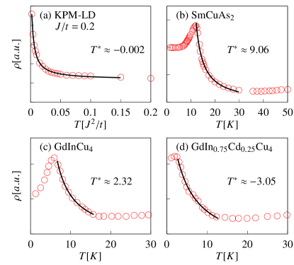
Figure S1: Fits (solid lines) to various resistivity data (circles) by Eq. (S12) with three parameters $\{a,b,T^{*}\}$. Data points are taken from: (a) KPM-LD results for triangular KLM with $J/t=0.2$ at filling $n=0.09$. (b) SmCuAs₂, from Ref. Sampathkumaran et al. (2003). (c-d) GdIn_1-xCd_xCu₄, from Ref. Fritsch et al. (2006).

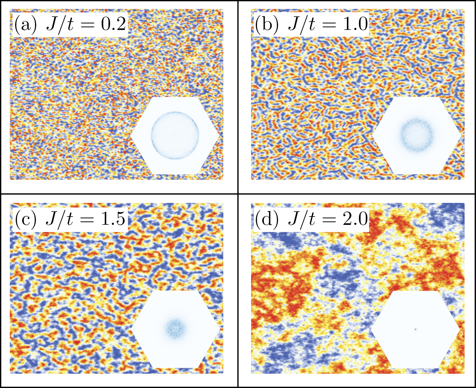
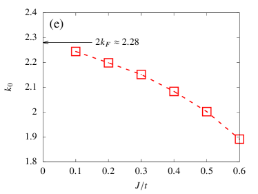
Figure S2: (a-d) Real-space fluctuations obtained from KPM-LD for a triangular KLM at filling fraction $n=0.09$ and temperature $T=0.002J^{2}/t$. The color gradient represents an arbitrary component of the spin 3-vector. Insets: corresponding $\mathcal{S}(\bm{k})$ in the 1st BZ. (e) KPM-LD results of momentum-space ring radius $k_{0}$ as a function of $J/t$, again with fixed parameters $n=0.09$ and temperature $T=0.002J^{2}/t$. (the dashed line is guide to the eye)

IV Spherical approximation

In the spherical approximation, the local constraint, $|\bm{S}_{i}|=1$, is replaced by a global one: $\sum_{i}|\bm{S}_{i}|^{2}=N$, where $N$ is the total number of sites. The partition function becomes:

$$\mathcal{Z} =\int\mathcal{D}\bm{S}d\lambda e^{-\beta\mathcal{H}-i\lambda\left(\sum_{i}|\bm{S}_{i}|^{2}-N\right)}$$

$$=\int\mathcal{D}\bm{S}d\lambda e^{-\beta\sum_{\bm{k}}\left[\Delta-J^{2}\tilde{\chi}_{\bm{k}}\right]|S_{\bm{k}}|^{2}},$$ (S14)

where $\lambda\equiv-i\beta\Delta$ is a Lagrangian multiplier introduced to enforce the global constraint. After integrating out the spins, we obtain the structure factor:

$${\cal S}({\bm{k}})=\frac{3T}{2[\Delta(T)-J^{2}{\tilde{\chi}}_{\bm{k}}]},$$ (S15)

where the parameter $\Delta(T)$ is determined by the self-consistency condition $\sum_{\bm{k}}|\bm{S}_{\bm{k}}|^{2}=\sum_{i}|\bm{S}_{i}|^{2}=N$, or equivalently

$$\frac{1}{N}\sum_{\bm{k}}\frac{J^{2}}{\Delta(T)-J^{2}{\tilde{\chi}}_{\bm{k}}}=\frac{2J^{2}\beta}{3}.$$ (S16)

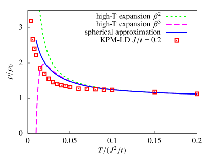
Figure S3: Temperature dependence of the resistivity for a triangular KLM at filling fraction $n=0.09$. The lines correspond to calculations based on the the Born approximation and a bare susceptibility with a renormalized wave-vector, $\chi^{0}_{k}\to\chi^{0}_{\alpha k}$, where the rescaling factor $\alpha$ is chosen to enforce the condition $k_{0}\simeq 2.2$ for $J/t=0.2$ . The symbols correspond to the results of KPM-LD simulations.

V Renormalization of Fermi wave-vector

In the weak-coupling limit $J/t\to 0$, the structure factor $\mathcal{S}(\bm{k})$ at low temperature is maximized at a ring with radius $k_{0}=2k_{F}$. However, as it is discussed in the main text, the ring shrinks towards the center of the 1st Brillouin zone upon increasing $J/t$. Correspondingly, in real space, we see the liquid-like phase with characteristic wavelength $2\pi/k_{0}$, which finally develops into ferromagnetism at large couplings $J/t\gtrsim 2$ [see Figs. S2 (a-d)].

To further illustrate this fact, we performed KPM-LD simulations on $256\times 256$ triangular lattice for $n=0.09$, $J/t=\{0.1,0.2,\ldots,0.6\}$ and a relatively low temperature $T/(J^{2}/t)=0.002$. The Chebyshev polynomial expansion order is $M=1000$ ($J/t=0.1$) and $M=500$ ($J/t=\{0.2,0.3,\ldots,0.6\}$). The number of random vectors is $R=512$ ($J/t=0.1$) and $R=128$ ($J/t=\{0.2,0.3,\ldots,0.6\}$). The numbers of total Langevin steps are $\{1\times 10^{4},3\times 10^{3}\}$ ($J/t=\{0.1,0.2\}$), and $5\times 10^{3}$ ($J/t=\{0.3,\ldots,0.6\}$), each of duration $\Delta\tau=100$ ($J/t=\{0.1,0.2\}$) and $\Delta\tau=10$ ($J/t=\{0.3,\ldots,0.6\}$). Then starting from the $2\times 10^{3}$th Langevin step, we average the value of $k_{0}$ for spin configurations differed by every $100$ Langevin steps.

As shown in Figs. 1(d)(f) of the main text, $k_{0}=2k_{F}$ ($k_{0}\approx 2.28$) in the weak-coupling limit, $J/t\to 0$. This result arises from the bare magnetic susceptibility maximum at $k=2k_{F}$ [see Fig. 1(b)]. However, Fig. S2(e) shows that $k_{0}$ decreases monotonically as a function of $J/t$. For $J/t=0.2$, the difference between $k_{0}$ and the bare $2k_{F}$ ($2k_{F}$ at $J/t=0$) is approximately equal to $0.08$. This shift of $k_{0}$ as a function of $J/t$ explains the low-temperature deviation between the analytical result for $\rho$, obtained in the weak-coupling limit, and the numerical result obtained for $J/t=0.2$ [see Fig. 2(a)]. To better illustrate this point, Fig. S3 shows a comparison between the analytical results based on a bare susceptibility function in which the wave-vector has been rescaled ($\chi^{0}_{k}\to\chi^{0}_{\alpha k}$) to enforce the condition $k_{0}\simeq 2.2$ for $J/t=0.2$. These clear improvement of the agreement between the analytical and the numerical result indicates that the shift in $k_{0}$, which is not captured at the RKKY level, is the main source of deviation between the resistivity curve, $\rho(T)$, for finite $J/t$ and the curve obtained in the weak-coupling limit $J/t\to 0$.

References

- Kondo (1964) J. Kondo, Prog. Theor. Phys. 32, 37 (1964).
- Hewson (1993) A. C. Hewson, The Kondo Problem to Heavy Fermions (Cambridge University Press, Cambridge, England, 1993).
- Mallik et al. (1998) R. Mallik, E. V. Sampathkumaran, M. Strecker, and G. Wortmann, Europhys. Lett. 41, 315 (1998).
- Sampathkumaran et al. (2003) E. V. Sampathkumaran, K. Sengupta, S. Rayaprol, K. K. Iyer, T. Doert, and J. P. F. Jemetio, Phys. Rev. Lett. 91, 036603 (2003).
- Sengupta et al. (2004) K. Sengupta, S. Rayaprol, E. Sampathkumaran, T. Doert, and J. Jemetio, Physica (Amsterdam) 348B, 465 (2004).
- Fritsch et al. (2005) V. Fritsch, J. D. Thompson, and J. L. Sarrao, Phys. Rev. B 71, 132401 (2005).
- Fritsch et al. (2006) V. Fritsch, J. D. Thompson, J. L. Sarrao, H.-A. Krug von Nidda, R. M. Eremina, and A. Loidl, Phys. Rev. B 73, 094413 (2006).
- (8) The “metallicity parameter” is not particularly large in these compounds (for example, in Ref. Nakatsuji et al., 2006), and one could in principle invoke localization as an explanation of the resistivity upturn. However, the fact that the resistivity maximum occurs at the ordering temperature points to the magnetic nature of the effect.
- Note (1) Commonly, the magnetic correlation length is on the order of the lattice spacing at the Curie-Weiss temperature. However, it may develop at higher temperatures in materials with competing ferro- and antiferromagnetic interactions. In this Letter, we define as the temperature at which becomes equal to the lattice spacing.
- Liu et al. (1987) F.-s. Liu, W. A. Roshen, and J. Ruvalds, Phys. Rev. B 36, 492 (1987).
- Ruvalds and Sheng (1988) J. Ruvalds and Q. G. Sheng, Phys. Rev. B 37, 1959 (1988).
- Oitmaa et al. (2006) J. Oitmaa, C. Hammer, and W. Zheng, Series Expansion Methods for Strongly Interacting Lattice Models (Cambridge University Press, Cambridge, England, 2006).
- Stanley (1968) H. E. Stanley, Phys. Rev. 176, 718 (1968).
- Conlon and Chalker (2010) P. H. Conlon and J. T. Chalker, Phys. Rev. B 81, 224413 (2010).
- Weiße et al. (2006) A. Weiße, G. Wellein, A. Alvermann, and H. Fehske, Rev. Mod. Phys. 78, 275 (2006).
- Barros and Kato (2013) K. Barros and Y. Kato, Phys. Rev. B 88, 235101 (2013).
- Barros et al. (2014) K. Barros, J. W. F. Venderbos, G.-W. Chern, and C. D. Batista, Phys. Rev. B 90, 245119 (2014).
- Kubo (1957) R. Kubo, J. Phys. Soc. Jpn. 12, 570 (1957).
- Note (2) Whether the resistivity drops or increases below depends on the competition of this effect and the reduction of the number of carriers due to the opening of a gap at the Fermi level. The resistivity behavior at is described in Ref. Fisher and Langer (1968).
- Note (3) Exceptions are fine-tuned systems with flat bands or lines of global maxima or minima of .
- (21) See Supplemental Material for the perturbation calculation of the resistivity for the KLM, the sign dependence of the inverse relaxation time, the temperature dependence of , the derivation of the spherical approximation, and the renormalization of the structure factor ring radius .
- (22) The data point at is accurate to order . The primary sources of error are the finite and the incomplete equilibration at this lowest temperature data point.
- Note (4) All lists of parameters in this paragraph correspond to the four values of in the parentheses.
- Mentink et al. (2010) J. H. Mentink, M. V. Tretyakov, A. Fasolino, M. I. Katsnelson, and T. Rasing, J. Phys. Condens. Matter 22, 176001 (2010).
- Tang and Saad (2012) J. M. Tang and Y. Saad, Numerical Linear Algebra with Applications 19, 485 (2012).
- Bastin et al. (1971) A. Bastin, C. Lewiner, O. Betbeder-matibet, and P. Nozieres, J. Phys. Chem. Solids 32, 1811 (1971).
- García et al. (2015) J. H. García, L. Covaci, and T. G. Rappoport, Phys. Rev. Lett. 114, 116602 (2015).
- Note (5) For , the first three data points at low temperature are expanded up to .
- Note (6) Except for cases when the electron-spin scattering is either too strong or too weak in comparison to the other scattering channels.
- Note (7) The only difference is that the prefactors of become now functions of .
- Udagawa et al. (2012) M. Udagawa, H. Ishizuka, and Y. Motome, Phys. Rev. Lett. 108, 066406 (2012).
- Chern et al. (2013) G.-W. Chern, S. Maiti, R. M. Fernandes, and P. Wölfle, Phys. Rev. Lett. 110, 146602 (2013).
- Matsukura et al. (1998) F. Matsukura, H. Ohno, A. Shen, and Y. Sugawara, Phys. Rev. B 57, R2037 (1998).
- Jungwirth et al. (2006) T. Jungwirth, J. Sinova, J. Mašek, J. Kučera, and A. H. MacDonald, Rev. Mod. Phys. 78, 809 (2006).
- Salamon and Jaime (2001) M. B. Salamon and M. Jaime, Rev. Mod. Phys. 73, 583 (2001).
- Nakatsuji et al. (2006) S. Nakatsuji, Y. Machida, Y. Maeno, T. Tayama, T. Sakakibara, J. van Duijn, L. Balicas, J. N. Millican, R. T. Macaluso, and J. Y. Chan, Phys. Rev. Lett. 96, 087204 (2006).
- Fisher and Langer (1968) M. E. Fisher and J. S. Langer, Phys. Rev. Lett. 20, 665 (1968).