ALGORITHMIC COMPUTATION OF POLYNOMIAL AMOEBAS

Abstract

We present algorithms for computation and visualization of amoebas, their contours, compactified amoebas and sections of three-dimensional amoebas by two-dimensional planes. We also provide a method and an algorithm for the computation of polynomials whose amoebas exhibit the most complicated topology among all polynomials with a fixed Newton polytope. The presented algorithms are implemented in computer algebra systems Matlab 8 and Mathematica 9.

1 Introduction

The amoeba of a multivariate polynomial in several complex variables is the Reinhardt diagram of its zero locus in the logarithmic scale with respect to each of the variables [16]. The term <<amoeba>> has been coined in [5, Chapter 6] where two competing definition of the amoeba of a polynomial have been given: the affine and the compactified versions. Both definitions are only interesting in dimension two and higher since the amoeba of a univariate polynomial is a finite set that can be explored by a variety of classical methods of localization of polynomial roots.

The geometry of the amoeba of a polynomial carries much information on the zeros of this polynomial and is closely related to the combinatorial structure of its Newton polytope (see Theorem 2.1). Despite loosing half of the real dimensions, the image of the zero locus of a polynomial in the amoeba space reflects the relative size of some of its coefficients.

From the computational point of view, the problem of giving a complete geometric or combinatorial description of the amoeba of a polynomial is a task of formidable complexity [10], despite the substantial recent progress in this direction [12, 13, 11]. The number of connected components of an amoeba complement as a function of the coefficients of the polynomial under study is still to be explored by means of the modern methods of computer algebra. In particular, the conjecture by M.Passare on the solidness of maximally sparse polynomials (see Definition 5) remains open for a long time.

Amoebas can be computed and depicted by means of a variety of approaches and methods (see [3, 10, 8, 12, 6, 13] and the references therein). The present paper is meant to move forward the art of computing and drawing complex amoebas of algebraic hypersurfaces. A special attention paid to the geometrically most interesting and computationally most challenging case of optimal hypersurfaces (see Definition 4). We expose methods and algorithms for computation and visualization of amoebas of bivariate polynomials, their contours and compactified versions. The developed algorithms are used in higher dimensions for depicting sections of amoebas of polynomials in three variables. The main focus of the paper is on polynomials whose amoebas have the most complicated topological structure among all polynomials with a given Newton polytope (see Definition 4). We provide an algorithm for explicit construction of such polynomials.

The presented algorithms are implemented in the computer algebra systems Matlab 8 (64-bit) and Wolfram Mathematica 9 (64-bit). All examples in the paper have been computed on Intel Core i5-4440 CPU clocked at 3.10 GHz with 16 Gb RAM under MS Windows 7 Ultimate SP1.

2 CONVEX POLYTOPES, CONES AND AMOEBAS: DEFINITIONS AND PRELIMINARIES

Let $p\left(x\right)$ be a polynomial in $n$ complex variables:

$$p\left(x_{1},\ldots,x_{n}\right)=\sum_{\alpha\in A}c_{\alpha}x^{\alpha}=\sum_{\alpha\in A}c_{\alpha_{1}\ldots\alpha_{n}}x_{1}^{\alpha_{1}}\cdot\ldots\cdot x_{n}^{\alpha_{n}},$$

where $A\subset\mathbb{Z}^{n}$ is a finite set.

Definition 1

The Newton polytope $\mathcal{N}_{p\left(x\right)}$ of a polynomial $p\left(x\right)$ is the convex hull of the set $A$ of its exponent vectors.

Definition 2

The recession cone of a convex set $M$ is the set-theoretical maximal element in the family of convex cones whose shifts are contained in $M$.

Definition 3

The amoeba $\mathcal{A}_{p\left(x\right)}$ of a polynomial $p\left(x\right)$ is the image of its zero locus under the map

$$\mathrm{Log}:\;\left(x_{1},\ldots,x_{n}\right)\longmapsto\left(\ln\left|x_{1}\right|,\ldots,\ln\left|x_{n}\right|\right).$$

The connected components of the complement to the amoeba $\mathcal{A}_{p\left(x\right)}$ are convex and in bijective correspondence with the expansions of the rational function $1/p(x)$ into Laurent series centered at the origin [4]. The next statement shows how the Newton polytope $\mathcal{N}_{p\left(x\right)}$ is reflected in the geometry of the amoeba $\mathcal{A}_{p\left(x\right)}$ [4, Theorem 2.8 and Proposition 2.6].

Theorem 2.1

(See [4].) Let $p\left(x\right)$ be a Laurent polynomial and let $\left\{M\right\}$ denote the family of connected components of the amoeba complement ${}^{c}\!\mathcal{A}_{p\left(x\right)}$. There exists an injective function $\nu:\{M\}\rightarrow\mathbb{Z}^{n}\cap\mathcal{N}_{p\left(x\right)}$, such that the cone that is dual to the polytope $\mathcal{N}_{p\left(x\right)}$ at the point $\nu\left(M\right)$ coincides with the recession cone of $M$. In particular, the number of connected components of ${}^{c}\!\mathcal{A}_{p\left(x\right)}$ cannot be smaller than the number of vertices of the polytope $\mathcal{N}_{p\left(x\right)}$ and cannot exceed the number of integer points in $\mathcal{N}_{p\left(x\right)}$.

Thus the amoeba of polynomial $p(x)$ in $n\geqslant 2$ variables is a closed connected unbounded subset of $\mathbb{R}^{n}$ whose complement consists of a finite number of convex connected components. Besides, a two-dimensional amoeba has <<tentacles>> that go off to infinity in the directions that are orthogonal to the sides of the polygon $\mathcal{N}_{p\left(x\right)}$ (see Fig. 3.1, 3.2, 4.1).

The two extreme values for the number of connected components of an amoeba complement are of particular interest.

Definition 4

(See [4, Definition 2.9].) An algebraic hypersurface $\mathcal{H}\subset(\mathbb{C}^{*})^{n}$, $n\!\geqslant\!2$, is called optimal if the number of connected components of the complement of its amoeba ${}^{c}\!\mathcal{A}_{\mathcal{H}}$ equals the number of integer points in the Newton polytope of the defining polynomial for $\mathcal{H}$. We will say that a polynomial (as well as its amoeba) is optimal if its zero locus is an optimal algebraic hypersurface.

In other words, an algebraic hypersurface is optimal if the topology of its amoeba is as complicated as it could possibly be under the condition that the Newton polytope of the defining polynomial is fixed. The other extreme case of the topologically simplest possible amoeba is defined as follows.

Definition 5

(See [9].) An algebraic hypersurface $\mathcal{H}\subset(\mathbb{C}^{*})^{n}$, $n\geqslant 2$, is called solid, if the number of connected components of its amoeba complement ${}^{c}\!\mathcal{A}_{\mathcal{H}}$ equals the number of vertices of the Newton polytope of its defining polynomial $\mathcal{H}$.

Thus the solid and the optimal amoebas are the endpoints of the spectrum of amoebas of polynomials with a given Newton polytope. Of course there exist plenty of optimal (as well as solid) amoebas defined by polynomials with a given Newton polytope. In fact, both sets of amoebas regarded as subsets in the complex space of coefficients of defining polynomials, have nonempty interior.

In the bivariate case, an amoeba is solid if and only if all of the connected components of its complement are unbounded and no its tentacles are parallel. A two-dimensional optimal amoeba has, on the contrary, the maximal possible number of bounded connected components in its complement and the maximal possible number of parallel tentacles.

The functional dependency of the topological type of the amoeba $\mathcal{A}_{p\left(x\right)}$ on the coefficient of its defining polynomial $p\left(x\right)$ is complex and little understood at the present moment. A sufficient condition for the amoeba of a polynomial to be optimal is that it satisfies a <<natural>> system of partial differential equations of hypergeometric type [1, 2] while the support of the polynomial in question is complex enough [14]. In Section 4 we expose an algorithm for the computation of the hypergeometric polynomial with the prescribed Newton polytope.

Example 1

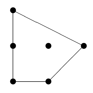
Let $\mathcal{N}$ denote the convex hull of the set of lattice points $\{\left(0,0\right),\left(1,0\right),$ $\left(0,2\right),\left(2,1\right)\}$, see Fig. 2.1. This polygon will appear in several examples that follow and has been chosen as one of the simplest polygons that contain an inner integer point as well as an integer point in the relative interior of its edge.

Figure 2.1: The support of the polynomials in Example 1

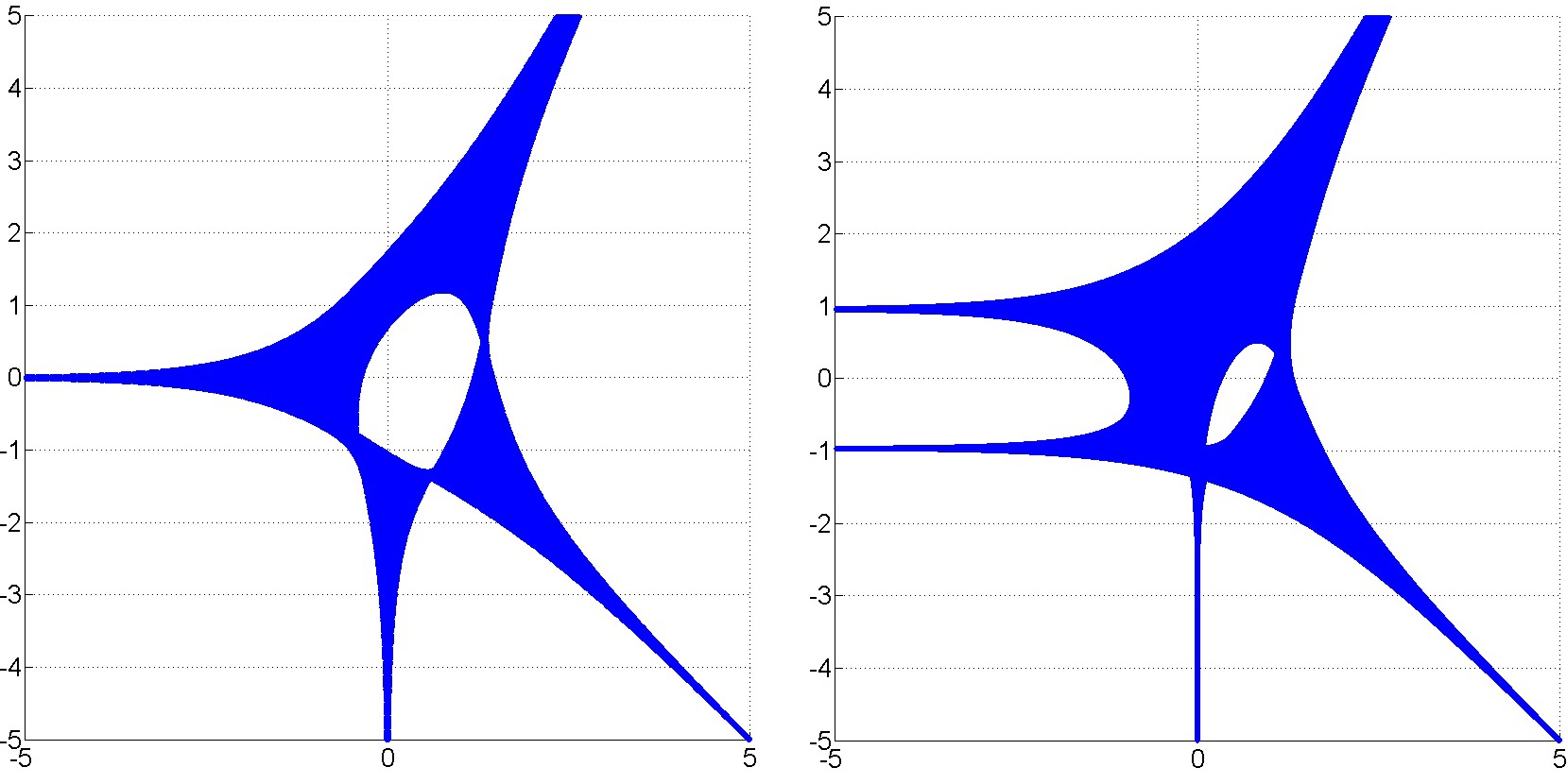
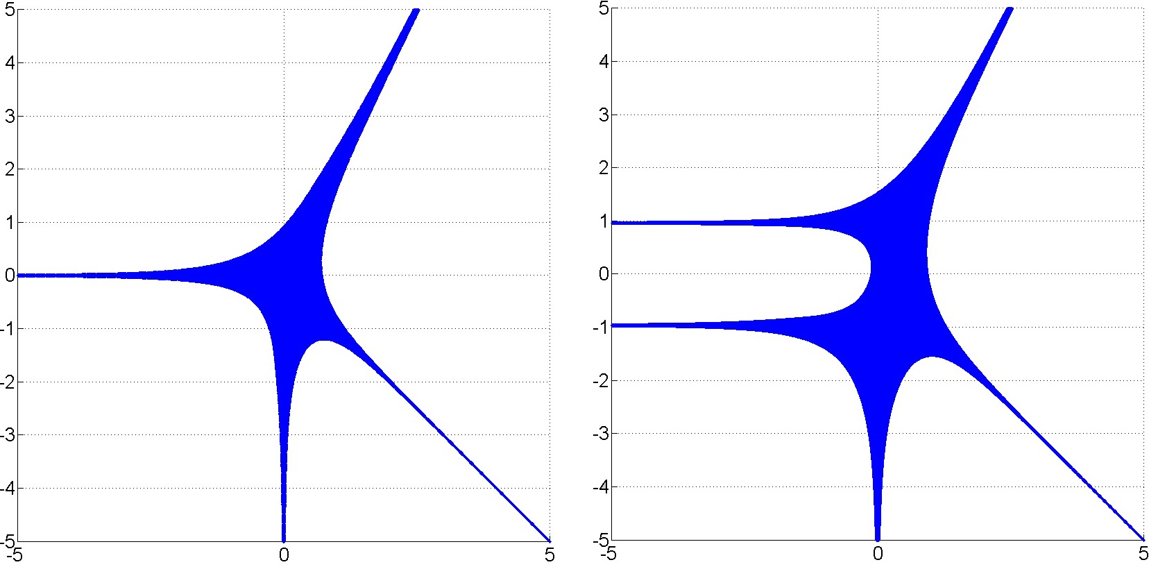
Fig. 3.1 and 3.2 show the amoebas of the four bivariate polynomials $p_{1}\left(x,y\right)=1+x+y+xy+y^{2}+x^{2}y$, $p_{2}\left(x,y\right)=1+x+3y+xy+y^{2}+x^{2}y$, $p_{3}\left(x,y\right)=1+x+y+4xy+y^{2}+x^{2}y$, $p_{4}\left(x,y\right)=1+x+3y+4xy+y^{2}+x^{2}y$ whose Newton polygons coincide with $\mathcal{N}$. The complement of the solid amoeba in Fig. 3.1 (left) consists of the four unbounded connected components with two-dimensional recession cones. The complement to the optimal amoeba in Fig. 3.2 (right) comprises six connected components: the four unbounded components with the two-dimensional recession cones, one unbounded component between the tentacles with the one-dimensional recession cone and the bounded component. The other two amoebas depicted in Fig. 3.1 (right) and 3.2 (left) exhibit five connected components in their respective complements and topologically assume an intermediate position between the solid and the optimal amoebas defined by polynomials with the Newton polygon $\mathcal{N}$.

The existing analytic methods [4, 11] do not in general allow one to predict the topological type of a polynomial with generic coefficients. From the computational point of view the tasks of depicting the amoebas in Fig. 3.1 and 3.2 are rather similar. Yet, to predict the existence of a bounded connected component of a given order [4] in an amoeba complement by means of analytic methods is in general a task of formidable complexity [10].

3 COMPUTING TWO-DIMENSIONAL AMOEBAS

Definition 6

We will call the <<carcase>> of an amoeba $\mathcal{A}$ any subset of $\mathcal{A}$, such that the number of connected components of the complement to the intersection $\mathcal{A}\cap B$ for a sufficiently large ball $B$ is as big as it could possibly be (that is, equal to the number of connected components in the complement of $\mathcal{A}$ in $\mathbb{R}^{n}$).

We remark that the carcase of an amoeba is not uniquely defined. However, the topology of its complement in a sufficiently big ball is well-defined and is as complex as possible. When speaking of depicting an amoeba we will mean depicting its suitable carcase.

In this section we consider bivariate polynomials of the form $p\left(x,y\right)=\sum c_{ij}x^{i}y^{j}$, $i=0,\ldots,m$, $j=0,\ldots,n$ and provide an algorithm for computing their amoebas.

Theorem 2.1 yields that the geometry of the amoeba $\mathcal{A}_{p}$ is closely related to the properties of the Newton polytope $\mathcal{N}_{p}$ of the polynomial $p$. Yet, the coefficients of $p$ also play a role and determine the size of the carcase of the amoeba in question. In what follows, the boundary of the domain where the carcase of an amoeba is depicted has been determined experimentally.

The next straightforward algorithm which computes the amoeba of a bivariate polynomial has been used by numerous authors in various forms [3, 8, 6]. We include it for the sake of completeness and future reference.

Algorithm 1 Algorithm for computing the amoeba $\mathcal{A}_{p}$ of a bivariate polynomial

1:List of the polynomial coefficients cx_list, in $x$ by all monomials $y^{k}$, $k=0,\ldots,\deg_{y}p$; the boundaries of the rectangular domain in the logarithmic amoeba space $a$, $b$; the number of values of the absolute value $n_{r}$ and the angle $n{}_{\varphi}$ of the complex variable.

2:List of coordinates of points that belong to the amoeba carcase $z\_list$, $w\_list$.

3:procedure Amoeba2D(cx_list, $a$, $b$, $n_{r}$, $n_{\varphi}$)

4:     z_list := empty list

5:     w_list := empty list

6:     d := the number of elements in cx_list – 1

7:     1d := $\left(1,\ldots,1\right)\in\mathbb{R}^{d}$ $\triangleright$ the vector with $d$ units

8:     $h_{r}:=\left(\exp\left(b\right)-\exp\left(a\right)\right)/\left(n_{r}-1\right)$

9:     $h_{\varphi}:=2\pi/\left(n_{\varphi}-1\right)$

10:     for $r=\exp(a):\exp(b):h_{r}$ do

11:         for $\varphi=0:2\pi:h_{\varphi}$ do

12:              $x:=r*\exp\left(\sqrt{-1}*\varphi\right)$

13:              $y:=\mathrm{roots}(cx\_list)$ $\triangleright$ the vector of zeros of the polynomial with the coefficients $cx\_list$

14:              Add $\mathrm{Log}(\left|x\right|*1d)$ to $z\_list$

15:              Add $\mathrm{Log}(\left|y\right|)$ to $w\_list$

16:         end for

17:     end for

18:     return $\left\{z\_list,w\_list\right\}$

19:end procedure

To obtain a picture of good quality the steps of the Algorithm 1 are repeated with the variables $x$ and $y$ interchanged. The points with the computed coordinates are depicted in the same figure.

Example 2

For the polynomial $p_{4}\left(x,y\right)$ in Example 1 the lists of polynomial coefficients in the variables $x$ and $y$ are as follows: cx_list=$\{1,\>3+4x+x^{2},\>1+x\}$ and cy_list=$\{y,\>1+4y,\>1+3y+y^{2}\}$. The (carcase of the) amoeba is depicted in the rectangle $\left[-5,5\right]\times\left[-5,5\right]$. The number of values of the absolute value of a variable is $n_{r}=2000$ while the number of values of its argument is $n{}_{\varphi}=180$. Fig. 3.1 and Fig. 3.2 feature the amoebas of the polynomials in Example 1 computed by means of Algorithm 1.

Figure 3.1: The amoebas of the polynomials $p_{1}\left(x,y\right)$ and $p_{2}\left(x,y\right)$

Figure 3.2: The amoebas of the polynomials $p_{3}\left(x,y\right)$ and $p_{4}\left(x,y\right)$

The topologically more involved amoeba of the polynomial in Example 4 has been computed in a similar way.

4 GENERATING OPTIMAL POLYNOMIALS

In this section we employ the notion of a hypergeometric polynomial for the purpose of constructive generation of optimal amoebas. We will need the following auxiliary definition.

Definition 7

A formal Laurent series

$$\sum_{s\in\mathbb{Z}^{n}}\varphi\left(s\right)\,x^{s}$$ (4.1)

is called hypergeometric if for any $j=1,\ldots,n$ the quotient $\varphi(s+e_{j})/\varphi(s)$ is a rational function in $s=(s_{1},\ldots,s_{n}).$ Throughout the paper we denote this rational function by $P_{j}(s)/Q_{j}(s+e_{j}).$ Here ${\{e_{j}\}}_{j=1}^{n}$ is the standard basis of the lattice $\mathbb{Z}^{n}.$ By the support of this series we mean the subset of $\mathbb{Z}^{n}$ on which $\varphi(s)\neq 0.$

A hypergeometric function is a (multi-valued) analytic function obtained by means of analytic continuation of a hypergeometric series with a nonempty domain of convergence along all possible paths.

Theorem 4.1

(Ore, Sato, cf [15]) The coefficients of a hypergeometric series are given by the formula

$$\varphi\left(s\right)=t^{s}\,U\left(s\right)\,\prod_{i=1}^{m}\Gamma\left(\left\langle{\bf A}_{i},s\right\rangle+c_{i}\right),$$ (4.2)

where $t^{s}=t_{1}^{s_{1}}\ldots t_{n}^{s_{n}}$, $t_{i},c_{i}\in\mathbb{C}$, ${\bf A}_{i}=\left(A_{i,1},\ldots,A_{i,n}\right)\in\mathbb{Z}^{n}$, $i=1,\ldots,m$ and $U\left(s\right)$ is the product of a certain rational function and a periodic function $\phi\left(s\right)$ such that $\phi\left(s+e_{j}\right)=\phi\left(s\right)$ for every $j=1,\ldots,n$.

Given the above data ($t_{i},c_{i},{\bf A}_{i},U\left(s\right)$) that determines the coefficient of a multivariate hypergeometric Laurent series, it is straightforward to compute the rational functions $P_{i}\left(s\right)/Q_{i}\left(s+e_{i}\right)$ using the $\Gamma$-function identity.

Definition 8

A (formal) Laurent series $\sum_{s\in\mathbb{Z}^{n}}\varphi\left(s\right)x^{s}$ whose coefficient satisfies the relations $\varphi(s+e_{j})/\varphi\left(s\right)=P_{j}\left(s\right)/Q_{j}\left(s+e_{j}\right)$ is a (formal) solution to the following system of partial differential equations of hypergeometric type:

$$x_{j}P_{j}\left(\theta\right)f\left(x\right)=Q_{j}\left(\theta\right)f\left(x\right),\,\,\,j=1,\ldots,n.$$ (4.3)

Here $\theta=\left(\theta_{1},\ldots,\theta_{n}\right)$, $\theta_{j}=x_{j}\frac{\partial}{\partial x_{j}}$.

The system (4.3) will be referred to as the Horn hypergeometric system defined by the Ore-Sato coefficient $\varphi(s)$ (see [2]) and denoted by ${\rm Horn}\left(\varphi\right)$.

In the present paper we will only consider the important special case of an Ore-Sato coefficient (4.2) with $t_{i}=1$ for all $i=1,\ldots,n$ and $U\left(s\right)\equiv 1$. The Horn system associated with such an Ore-Sato coefficient will be denoted by ${\rm Horn}\left(A,c\right)$, where $A$ is the matrix with the rows ${\bf A}_{1},\ldots,{\bf A}_{m}\in\mathbb{Z}^{n}$ and $c=\left(c_{1},\ldots,c_{m}\right)\in\mathbb{C}^{m}$. In this case the operators $P_{j}\left(\theta\right)$ and $Q_{j}\left(\theta\right)$ explicitly determine the system (4.3):

$$P_{j}\left(s\right)=\prod_{i:A_{i,j}>0}\prod_{\ell_{j}^{(i)}=0}^{A_{i,j}-1}\left(\left\langle{\bf A}_{i},s\right\rangle+c_{i}+\ell_{j}^{\left(i\right)}\right),$$

$$Q_{j}\left(s\right)=\prod_{i:A_{i,j}<0}\prod_{\ell_{j}^{(i)}=0}^{|A_{i,j}|-1}\left(\left\langle{\bf A}_{i},s\right\rangle+c_{i}+\ell_{j}^{\left(i\right)}\right).$$

For a convex integer polytope $\mathcal{N},$ we construct the list $B$ of the outer normals to the faces of $\mathcal{N}.$ We denote the length of this list by $q$. We assume the elements of $B$ to be normalized so that the coordinates of each outer normal are integer and relatively prime. Define the Ore-Sato coefficient

$$\varphi\left(s\right)=\frac{1}{\prod\limits_{j=1}^{q}\Gamma\left(1-\left\langle B_{j},s\right\rangle-c_{j}\right)}.$$ (4.4)

The hypergeometric system (4.3) defined by the Ore-Sato coefficient $\varphi(s)$ admits a polynomial solution with several interesting properties. Under some additional assumptions it turns out to have an optimal amoeba. We will employ the following algorithm to generate optimal polynomials of hypergeometric type.

Algorithm 2 Generation of a bivariate hypergeometric polynomial and its defining system of equations

1:List of vertices $N\_list$ of a convex integer polygon $P$.

2:List of coefficients $c\_list$ of the hypergeometric polynomial $p\left(x,y\right)$ whose Newton polygon is $P$.

3:procedure Hyperpoly2D(N_list)

4:     $B$ = list of outer normals to the sides of $P$.

5:     $\varphi\left(s,t\right)=1/\prod\limits_{j=1}^{q}\Gamma\left(1-\left\langle B_{j},\left(s,t\right)\right\rangle-c_{j}\right)$

6:     $c\_list$ = list of the coefficients of the hypergeometric polynomial

7:     $R_{1}=\mathrm{FunctionExpand}[\varphi\left(s+1,t\right)/\varphi\left(s,t\right)]$

8:     $R_{2}=\mathrm{FunctionExpand}[\varphi\left(s,t+1\right)/\varphi\left(s,t\right)]$

9:     $P_{1}=\mathrm{Numerator}[R_{1}]$

10:     $P_{2}=\mathrm{Numerator}[R_{2}]$

11:     $Q_{1}=\mathrm{Denumerator}[R_{1}]$

12:     $Q_{2}=\mathrm{Denumerator}[R_{2}]$

13:     $\theta_{x}=x\frac{dp}{dx}$

14:     $\theta_{y}=y\frac{dp}{dy}$

15:     $p$ = the polynomial defined by $c\_list$

16:     if $xP_{1}(\theta)p=Q_{1}(\theta)p$ and $yP_{2}(\theta)p=Q_{2}(\theta)p$ then

17:         return $\left\{c\_list\right\}$

18:     end if

19:end procedure

Example 3

The outer normals (normalized as explained above) to the sides of the polygon shown in Fig. 2.1 are as follows: $\left(0,-1\right)$, $\left(-1,0\right)$, $\left(1,2\right)$, $\left(1,-1\right)$. Using (4.4) we obtain

$$\begin{array}[]{c}\varphi\left(s,t\right)=(\Gamma\left(s+1\right)\Gamma\left(t+1\right)\Gamma\left(-s-2t+5\right)\Gamma\left(-s+t+2\right))^{-1}.\end{array}$$

By Definition 8 the above Ore-Sato coefficient $\varphi\left(s,t\right)$ gives rise to the polynomials

$$\begin{array}[]{c}P_{1}\left(s,t\right)=\left(-s-2t+4\right)\left(-s+t+1\right),\quad Q_{1}\left(s,t\right)=s+2,\\ P_{2}\left(s,t\right)=\left(s+2t-4\right)\left(s+2t-3\right),\quad Q_{2}\left(s,t\right)=\left(t+2\right)\left(-s+t+3\right).\end{array}$$

The corresponding hypergeometric system is defined by the linear partial differential operators

$$\left\{\begin{array}[]{l}x\,\left(-\theta_{x}-2\theta_{y}+4\right)\left(-\theta_{x}+\theta_{y}+1\right)-\left(\theta_{x}+2\right),\\ y\,\left(\theta_{x}+2\theta_{y}-4\right)\left(\theta_{x}+2\theta_{y}-3\right)-\left(\theta_{y}+2\right)\left(-\theta_{x}+\theta_{y}+3\right).\end{array}\right.$$ (4.5)

It is straightforward to check that the hypergeometric polynomial $p(x,y)=1+4x+6y+24xy+12x^{2}y+2y^{2}$ belongs to the kernels of the operators (4.5).

Example 4

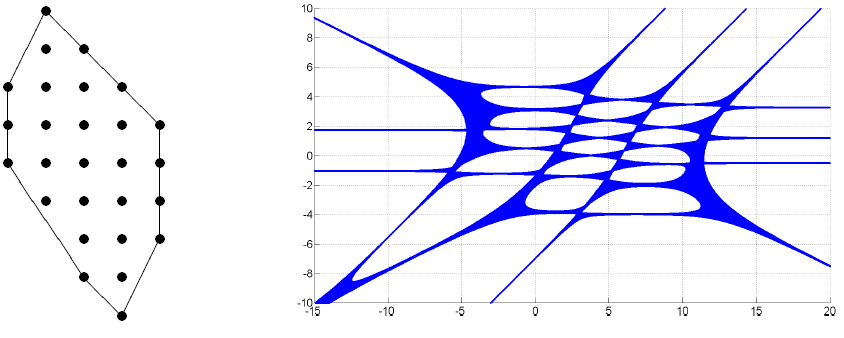
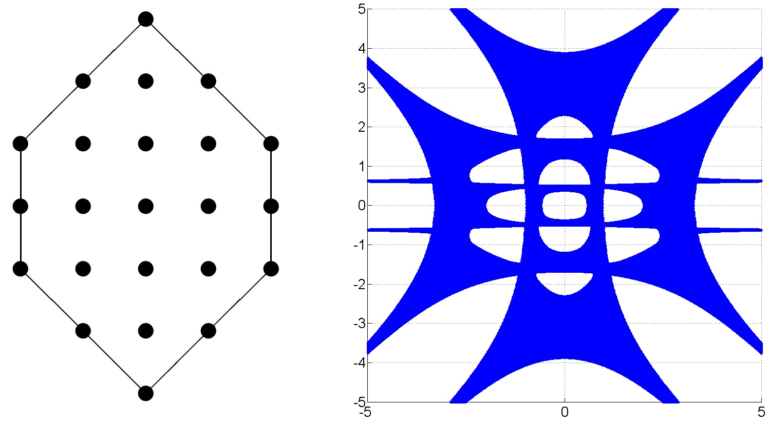
Using Algorithms 1 and 2 we compute the coefficients of the hypergeometric polynomial supported in the polygon $\mathcal{N}_{p_{h}\left(x,y\right)}$ shown in Fig. 4.1 (left): $p_{h}\left(x,y\right)=2x^{2}+20xy+72x^{2}y+20x^{3}y+5y^{2}+160xy^{2}+450x^{2}y^{2}+160x^{3}y^{2}+5x^{4}y^{2}+12y^{3}+300xy^{3}+800x^{2}y^{3}+300x^{3}y^{3}+12x^{4}y^{3}+5y^{4}+160xy^{4}+450x^{2}y^{4}+160x^{3}y^{4}+5x^{4}y^{4}+20xy^{5}+72x^{2}y^{5}+20x^{3}y^{5}+2x^{2}y^{6}.$ The amoeba $\mathcal{A}_{p_{h}\left(x,y\right)}$ of this polynomial is depicted in Fig. 4.1 (right).

A more involved hypergeometric polynomial is given by $p_{h2}(x,y)=-456456x^{3}+488864376x^{2}y-28756728x^{3}y+25420947552x^{2}y^{2}-244432188x^{3}y^{2}+3003x^{4}y^{2}-119841609888xy^{3}+127104737760x^{2}y^{3}-465585120x^{3}y^{3}+6006x^{4}y^{3}+1396755360y^{4}-508418951040xy^{4}+139815211536x^{2}y^{4}-232792560x^{3}y^{4}+1729x^{4}y^{4}+4190266080y^{5}-355893265728xy^{5}+41611670100x^{2}y^{5}-29628144x^{3}y^{5}+57x^{4}y^{5}+698377680y^{6}-58663725120xy^{6}+3328933608x^{2}y^{6}-705432x^{3}y^{6}-2327925600xy^{7}+55023696x^{2}y^{7}-16930368xy^{8}.$ Its defining Ore-Sato coefficient equals $\varphi(s,t)=\Gamma(s+t-4)\Gamma(-4s+t-16)\Gamma(-3s-2t-5)\Gamma(3s-t-3)\Gamma(2s+t-5).$ The amoeba of this polynomial is shown in Fig. 4.2.

Figure 4.1: The Newton polytope and the amoeba of the hypergeometric polynomial $p_{h}\left(x,y\right)$

Figure 4.2: The Newton polytope and the amoeba of the hypergeometric polynomial $p_{h2}\left(x,y\right)$

5 COMPUTING CONTOURS OF AMOEBAS OF BIVARIATE POLYNOMIALS

The boundary of an amoeba admits a rich analytic structure that is revealed in the following definition.

Definition 9

The contour of the amoeba $\mathcal{A}_{p\left(x\right)}$ is the set $\mathcal{C}_{p\left(x\right)}$ of critical points of the logarithmic map $\mathrm{Log}$ restricted to the zero locus of the polynomial $p\left(x\right)$:

$$\mathrm{Log}:\;\left\{p\left(x\right)=0\right\}\rightarrow\mathbb{R}^{n}.$$

The structure of the contour of an amoeba can be described in terms of the logarithmic Gauss map which is defined as follows.

Definition 10

Denote by $\mathrm{Gr}(n,k)$ the Grassmannian of $k$-dimensional subspaces in $\mathbb{C}^{n}$. The logarithmic Gauss map [7] is defined to be the map $\gamma:\;\mathcal{H}\longmapsto\mathrm{Gr}(n,k)$ that maps a regular point $x\in\mathrm{reg}\thinspace\mathcal{H}$ into the normal subspace $\gamma(x)$ to the image $\mathrm{log}\thinspace\mathcal{H}$.

The boundary of an amoeba $\partial\mathcal{A}_{p\left(x\right)}$ is necessarily a subset of the contour $\mathcal{C}_{p\left(x\right)}$ but is in general different from it.

Knowing the structure of the contour of an amoeba is important for describing the topological structure of the amoeba complement. Experiments show that a cusp of the contour inside the <<body>> of the corresponding amoeba is a counterpart of a missing connected component in its complement.

One of the ways to draw the contour of an amoeba is to depict the solutions to the system of algebraic equations

$$\begin{cases}p\left(x,y\right)=0,\\ x\frac{\partial p\left(x,y\right)}{\partial x}-uy\frac{\partial p\left(x,y\right)}{\partial y}=0.\end{cases}$$ (5.1)

Here $u\in\mathbb{R}\cup\left\{\infty\right\}$ is a real parameter that encodes the slope of the normal line to the contour of the amoeba.

Eliminating the variables $x$ and $y$ out of the system (5.1) we obtain polynomials $s\left(y,u\right)$ and $t\left(x,u\right)$ that can be used to depict the contour of the amoeba by means of the following algorithm.

Algorithm 3 Computing the contour $\mathcal{C}_{p}$ of the amoeba of a bivariate polynomial

1:List of polynomial coefficients cx_list cy_list depending on $u$, by all monomials $x^{k}$, $k=0,\ldots,\deg_{x}t$, $y^{m}$, $m=0,\ldots,\deg_{y}s$; initial value $u_{1}$, final value $u_{n}$ and the step $h_{u}$.

2:List of coordinates of points $z\_list$, $w\_list$ that belong to the contour of the amoeba.

3:procedure Contour2D(cx_list, cy_list, $u_{1}$, $u_{n}$, $h_{u}$)

4:     z_list := the empty list

5:     w_list := the empty list

6:     dx := the number of elements in cx_list – 1

7:     dy := the number of elements in cy_list – 1

8:     for $u=u_{1}:u_{n}:h_{u}$ do

9:         $x:=\mathrm{roots}(cx\_list)$ $\triangleright$ the vector of zeros of the polynomial with the coefficients $cx\_list$

10:         $y:=\mathrm{roots}(cy\_list)$ $\triangleright$ the vector of zeros of the polynomial with the coefficients $cy\_list$

11:         Add $\mathrm{Log}(\left|x\right|)$ to $z\_list$

12:         Add $\mathrm{Log}(\left|y\right|)$ to $w\_list$

13:     end for

14:     return $\left\{z\_list,w\_list\right\}$

15:end procedure

Remark 1

The lists of coordinates that are obtained at each iteration of the cycle in the above algorithm might contain additional elements that do not correspond to the amoeba contour. They are sorted out by checking against the system of equations (5.1).

Example 5

The system of equations (5.1) associated with the first polynomial in Example 1 has the form

$$\begin{cases}1+x+y+xy+y^{2}+x^{2}y=0,\\ x-uy+xy-uxy+2x^{2}y-ux^{2}y-2uy^{2}=0.\end{cases}$$

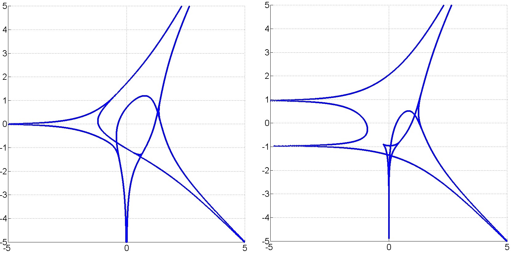
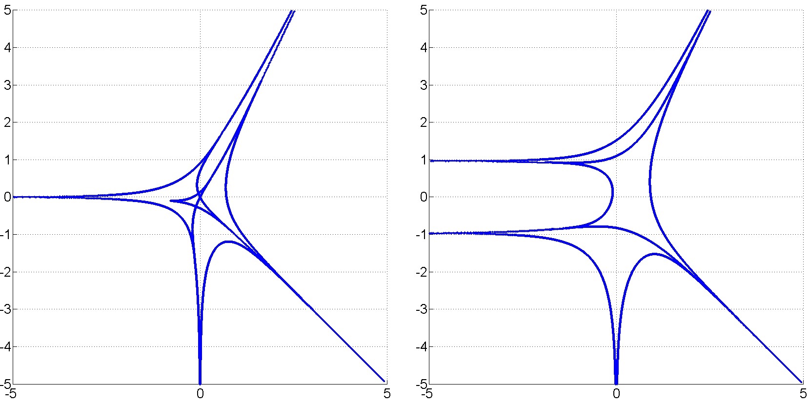
Eliminating variables $x$ and $y$ yields the equations $u-2uy+u^{2}y-4uy^{2}+2u^{2}y^{2}-2uy^{3}-u^{2}y^{3}+3uy^{4}+4uy^{5}+u^{2}y^{5}=1-y-4y^{2}-9y^{3}-7y^{4}-4y^{5}$ and $-3u^{2}-3ux-5u^{2}x-2ux^{2}+u^{2}x^{2}+3ux^{3}+5u^{2}x^{3}+2ux^{4}+3u^{2}x^{4}+ux^{5}+u^{2}x^{5}=x^{2}+2x^{3}+5x^{4}+2x^{5}$ respectively. The lists of the coefficients that depend on $u$ are cx_list = $\{-1+u,\>1-2u+u^{2},\>4-4u+2u^{2},\>9-2u-u^{2},\>7+3u,4+4u+u^{2}\}$ and cy_list = $\{-3u^{2},\>-3u-5u^{2},\>-1-2u+u^{2},\>-2+3u+5u^{2},\>-5+2u+3u^{2},\>-2+u+u^{2}\}$. The parameter $u$ assumes values in the interval $\left[-120,120\right]$ with the step $h_{u}=0,001$. The obtained contours of the amoebas of the polynomials in Example 1 have nontrivial structure and are shown in Fig. 5.1 and 5.2.

Figure 5.1: Contours of the amoebas of the polynomials $p_{1}\left(x,y\right)$ and $p_{2}\left(x,y\right)$

Figure 5.2: Contours of the amoebas of the polynomials $p_{3}\left(x,y\right)$ and $p_{4}\left(x,y\right)$

6 COMPUTING TWO-DIMENSIONAL COMPACTIFIED AMOEBAS

Definition 11

The compactified amoeba $\overline{\mathcal{A}}_{p\left(x\right)}$ of a polynomial $p\left(x\right)$ is defined to be the image of its zero locus under the mapping

$$M\left(x\right)=\frac{\sum\limits_{\alpha\in A}\alpha\cdot\left|x^{\alpha}\right|}{\sum\limits_{\alpha\in A}\left|x^{\alpha}\right|}=\frac{\sum\limits_{\left(\alpha_{1},\ldots,\alpha_{n}\right)\in A}\left(\alpha_{1},\ldots,\alpha_{n}\right)\cdot\left|x^{\alpha_{1}}\cdot\ldots\cdot x^{\alpha_{n}}\right|}{\sum\limits_{\left(\alpha_{1},\ldots,\alpha_{n}\right)\in A}\left|x^{\alpha_{1}}\cdot\ldots\cdot x^{\alpha_{n}}\right|}.$$ (6.1)

Numeric computation of two-dimensional compactified amoebas is similar to that of their affine counterparts (see Algorithm 1). The main computational issue is dealing with the moment map (6.1) instead of the logarithmic map into the affine space.

Example 6

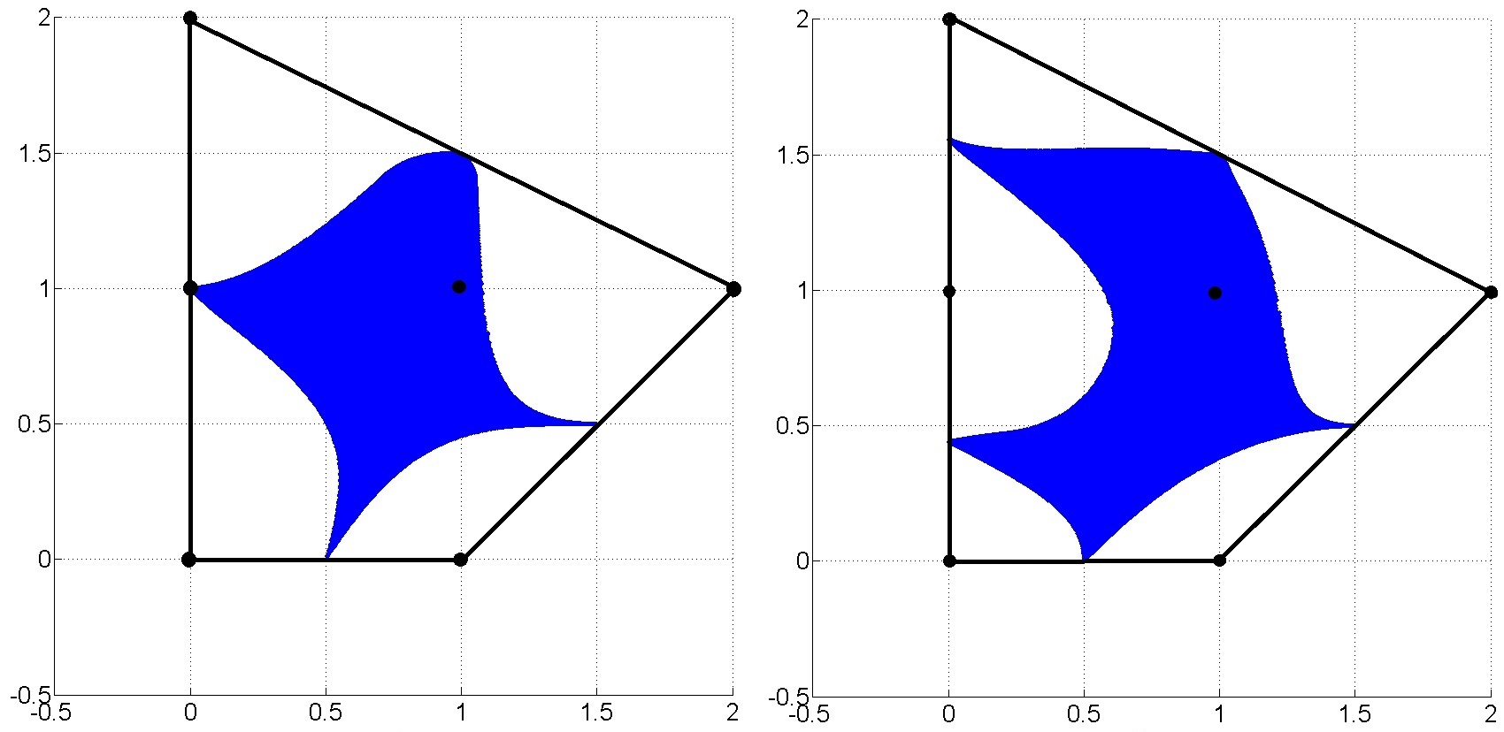
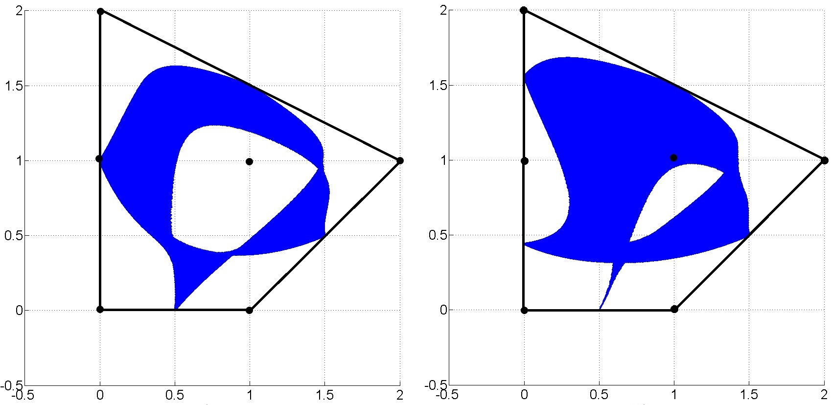
Applying (6.1) to the polynomials in Example 1 yields the mapping

$$\left(x,y\right)\longmapsto\mu\left(x,y\right)=$$

$$\frac{(1\cdot\left(0,0\right)+\left|x\right|\cdot\left(1,0\right)+\left|y\right|\cdot\left(0,1\right)+\left|xy\right|\cdot\left(1,1\right)+\left|y^{2}\right|\cdot\left(0,2\right)+\left|x^{2}y\right|\cdot\left(2,1\right))}{\left(\left|1\right|+\left|x\right|+\left|y\right|+\left|xy\right|+\left|y^{2}\right|+\left|x^{2}y\right|\right)}=$$

$$\frac{(\left|x\right|+\left|xy\right|+2\left|x^{2}y\right|,\left|y\right|+\left|xy\right|+2\left|y^{2}\right|+\left|x^{2}y\right|)}{\left(\left|1\right|+\left|x\right|+\left|y\right|+\left|xy\right|+\left|y^{2}\right|+\left|x^{2}y\right|\right)}.$$

The corresponding compactified amoebas inside the Newton polygon of their defining polynomials are shown in Fig. 6.1 and 6.2.

Figure 6.1: Compactified amoebas of the polynomials $p_{1}\left(x,y\right)$ and $p_{2}\left(x,y\right)$ in their Newton polygon

Figure 6.2: Compactified amoebas of the polynomials $p_{3}\left(x,y\right)$ and $p_{4}\left(x,y\right)$ in their Newton polygon

7 MULTIVARIATE OUTLOOK

Depicting three-dimensional amoebas represents a substantial computational challenge due to the complex geometry of their shape. We will now treat the problem of computing sections of amoebas of polynomials in three variables by two-dimensional hyperplanes.

Consider a polynomial in three complex variables $p\left(x,y,z\right)=\sum c_{ijk}x^{i}y^{j}z^{k}$, $i=0,\ldots,m$, $j=0,\ldots,n$, $k=0,\ldots,s$. To compute the section of its amoeba by the plane $\left|z\right|=\mathrm{const}$ we fix the absolute value of $z$ and modify Algorithm 1 by adding a cycle with respect to the values of the argument $\varphi_{z}\in\left[0;2\pi\right]$.

Algorithm 4 Computing section of the amoeba $\mathcal{A}_{p}$ of a polynomial in three variables

1:List of polynomial coefficients cxz_list, depending on $x$ and $z$ by all monomials $y^{k}$, $k=0,\ldots,\deg_{y}p$; bounds $a$, $b$ for the rectangular domain in the amoeba space where the amoeba section is depicted; the numbers $n_{r}$ and $n{}_{\varphi}$ of values of the absolute value and the argument of the variable $z\in\mathbb{C},$ respectively.

2:List of points that belong to the amoeba section $z\_list$, $w\_list$.

3:procedure Amoeba3D(cxz_list, $a$, $b$, $n_{r}$, $n_{\varphi}$, $z$)

4:     z_list := empty list

5:     w_list := empty list

6:     d := the number of elements in cxz_list – 1

7:     1d := $\left(1,\ldots,1\right)\in\mathbb{R}^{d}$ $\triangleright$ the vector of $d$ units

8:     $h_{r}:=\left(\exp\left(b\right)-\exp\left(a\right)\right)/\left(n_{r}-1\right)$

9:     $h_{\varphi}:=2\pi/\left(n_{\varphi}-1\right)$

10:     for $r=\exp(a):\exp(b):h_{r}$ do

11:         for $\varphi=0:2\pi:h_{\varphi}$ do

12:              $x:=r*\exp\left(\sqrt{-1}*\varphi\right)$

13:              $y:=\mathrm{roots}(cx\_list)$ $\triangleright$ the vector of zeros of the polynomial with the coefficients $cx\_list$

14:              Add $\mathrm{Log}(\left|x\right|*1d)$ to $z\_list$

15:              Add $\mathrm{Log}(\left|y\right|)$ to $w\_list$

16:         end for

17:     end for

18:     return $\left\{z\_list,w\_list\right\}$

19:end procedure

Example 7

Using the above Algorithm 4 we compute the section of the amoeba of the polynomial $p\left(x,y,z\right)=1+3y+y^{2}+6xy+x^{2}y+xyz+xyz^{2}$. This polynomial is one of the simplest polynomials with tetrahedral Newton polytopes that contain integer points in the interior as well as in the relative interior of faces of all positive dimensions (see Fig. 7.1).

Figure 7.1: The Newton polytope $\mathcal{N}_{p\left(x,y,z\right)}$

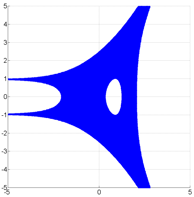
Figure 7.2: The section of the amoeba of the polynomial $p\left(x,y,z\right)$ by the plane $\log|z|=5$

The section of the amoeba $\mathcal{A}_{p\left(x,y,z\right)}$ by the plane $\log\left|z\right|=5$ is shown in Fig. 7.2.

Example 8

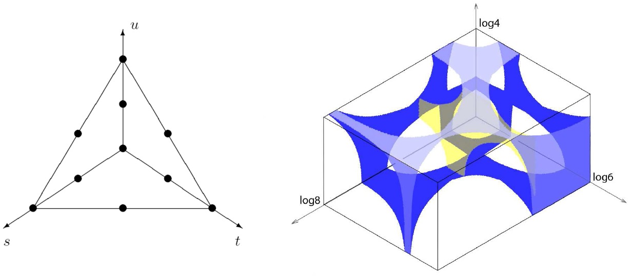
We now consider a computationally more challenging optimal hypergeometric polynomial in three variables supported in a regular integer octahedron. Due to symmetry it suffices to consider its part that belongs to the positive orthant and is shown in Fig. 7.3 (left). We use a three-dimensional version of Algorithm 2 to compute the corresponding (uniquely determined up to scaling) hypergeometric polynomial: $p_{h}\left(x,y,z\right)=x^{2}y^{2}+36x^{2}yz+36xy^{2}z+256x^{2}y^{2}z+36x^{3}y^{2}z+36x^{2}y^{3}z+x^{2}z^{2}+36xyz^{2}+256x^{2}yz^{2}+36x^{3}yz^{2}+y^{2}z^{2}+256xy^{2}z^{2}+1296x^{2}y^{2}z^{2}+256x^{3}y^{2}z^{2}+x^{4}y^{2}z^{2}+36xy^{3}z^{2}+256x^{2}y^{3}z^{2}+36x^{3}y^{3}z^{2}+x^{2}y^{4}z^{2}+36x^{2}yz^{3}+36xy^{2}z^{3}+256x^{2}y^{2}z^{3}+36x^{3}y^{2}z^{3}+36x^{2}y^{3}z^{3}+x^{2}y^{2}z^{4}$. Fig. 7.3 (right) shows the intersection of the amoeba $\mathcal{A}_{p_{h}\left(x,y,z\right)}$ with the three coordinate hyperplanes as well as with the hyperplanes $|x|=3,$ $|x|=8$, $|y|=6$, $|z|=4$ in the logarithmic amoeba space. The figure space is orthogonal to the vector $(1,1,1)$.

Figure 7.3: The part of the support of $p_{h}\left(x,y,z\right)$ that belongs to the positive orthant and the carcase of the corresponding part of the amoeba

Acknowledgements. The research was partially supported by the state order of the Ministry of Education and Science of the Russian Federation for Siberian Federal University (task 1.1462.2014/K, the second author), by Government of the Russian Federation (project no. 14.Y26.31.0006, the third author). and by the Russian Foundation for Basic Research, projects 15-31-20008-mol_a_ved (the second and the third authors), 15-01-00277-a and 14-01-00283-a (the second author).

References

• [1] Dickenstein, A., Sadykov, T. M.: Algebraicity of solutions to the Mellin system and its monodromy. Doklady Mathematics 75 (1), 80–82 (2007)
• [2] Dickenstein, A., Sadykov, T. M.: Bases in the solution space of the Mellin system. Sbornik Mathematics 198 (9-10), 1277–1298 (2007)
• [3] Forsberg, M.: Amoebas and Laurent Series. Doctoral Thesis presented at Royal Institute of Technology, Stockholm, Sweden. Bromma Tryck AB, ISBN 91-7170-259-8 (1998)
• [4] Forsberg, M., Passare, M., Tsikh, A. K.: Laurent determinants and arrangements of hyperplane amoebas. Adv. Math. 151, 45–70 (2000)
• [5] Gelfand, I. M., Kapranov, M. M., Zelevinsky, A. V.: Discriminants, resultants, and multidimensional determinants. Mathematics: Theory & Applications. Birkhäuser Boston, Inc., Boston, MA (1994)
• [6] Johansson, P.: On the Topology of the Coamoeba. Doctoral Thesis presented at Stockholm University, Sweden. US AB, ISBN 978-91-7447-933-1 (2014)
• [7] Kapranov, M. M.: A characterization of A-discriminantal hypersurfaces in terms of the logarithmic Gauss map. Math. Ann. 290, 277–285 (1991)
• [8] Nilsson, L.: Amoebas, Discriminants and Hypergeometric Functions. Doctoral Thesis presented at Stockholm University, Sweden. US AB, ISBN 978-91-7155-889-3 (2009)
• [9] Passare, M., Sadykov, T. M., Tsikh, A. K.: Nonconfluent hypergeometric functions in several variables and their singularities. Compos. Math. 141 (3), 787–810 (2005)
• [10] Purbhoo, K.: A Nullstellensatz for amoebas. Duke Math. J. 141 (3), 407–445 (2008)
• [11] Rullgård, H.: Stratification des espaces de polynômes de Laurent et la structure de leurs amibes (French). Comptes Rendus de l’Academie des Sciences - Series I: Mathematics 331 (5), 355–358 (2000)
• [12] Theobald, T.: Computing Amoebas. Experiment. Math. 11 (4), 513–526 (2002)
• [13] Theobald, T., de Wolff, T.: Amoebas of genus at most one. Adv. Math. 239, 190–213 (2013)
• [14] Sadykov, T. M., Tsikh, A. K.: Hypergeometric and Algebraic Functions in Several Variables (Russian). Nauka (2014)
• [15] Sadykov, T. M.: On a multidimensional system of hypergeometric differential equations. Siberian Mathematical Journal 39 (5), 986–997 (1998)
• [16] Viro, T.: What is an amoeba? Notices of the AMS 49 (8), 916–917 (2002)