Critical models above four dimensions: Small- solutions and stability
Abstract
We explore models in dimensions . Specifically, we investigate models of an vector field coupled to an additional scalar field via a cubic interaction. Recent results in have uncovered an interacting ultraviolet fixed point of the renormalization group (RG) if the number of components of the vector field is large enough, suggesting that these models are asymptotically safe. We set up a functional RG analysis of these systems to address three key issues: Firstly, we find that in the interacting fixed point exists all the way down to . Secondly, we show that the standard universality classes are actually embedded in those of the cubic models, in that the latter exhibit the same values for (most of) the critical exponents, but feature an additional third RG relevant direction. Thirdly, we address the critical question of global stability of the fixed-point potential to test whether the fixed point can underly a viable quantum field theory.
I Introduction: models within the asymptotic-safety paradigm
It has recently been suggested that a unitary UV completion of models above four dimensions can be found if the theory is formulated in terms of an vector field coupled to an additional scalar field, defined by the Lagrangian Fei:2014yja
| (1) |
with . The theory without the kinetic term for arises from a Hubbard-Stratonovich transformation of a pure quartic model with -component vector . The new field is introduced as a composite field representing the quadratic operator . In dimensions a perturbative renormalization group (RG) study has uncovered an UV fixed point with real values of the couplings for large enough Fei:2014yja ; Fei:2014xta . This provides a possible example of an asymptotically safe model. Asymptotic safety, proposed by Weinberg Weinberg:1980gg , has recently been explored as a new paradigm for quantum field theories Gies:2013pma ; Litim:2014uca , including quantum gravity Reuter:1996cp ; Codello:2008vh ; Benedetti:2009rx ; Falls:2013bv ; Becker:2014qya ; Dona:2013qba . At its heart lies an interacting fixed point, at which quantum fluctuations render the theory scale invariant. Further, the model defined by Eq. (1) is conjectured to be related to Vasiliev higher-spin theories Fradkin:1987ks ; Vasiliev:1990en ; Vasiliev:1992av ; Vasiliev:1995dn ; Vasiliev:1999ba ; Vasiliev:2003ev via the AdS/CFT correspondence Klebanov:2002ja ; Giombi:2014iua . It may thus provide a concrete connection between AdS/CFT and asymptotic safety.
Moreover, the model could provide a possible starting point to render the Higgs-Yukawa sector of the Standard Model asymptotically safe: While the issue of triviality represents an important unresolved problem in four dimensions Gies:2009hq ; Gies:2009sv ; Scherer:2009wu ; Vacca:2015nta , an UV fixed point in a setting with an additional compact dimension could provide a possible mechanism for UV completion.
Within the expansion, a stable111Here, “stable” refers to the number of RG relevant directions, not to the stability of the fixed-point potential. and real fixed point has been found only if , with the critical value being at one loop and on the level of the three-loop expansion Fei:2014xta . Using resummation techniques, a value of has been found on the four-loop level Gracey:2015tta . Conformal bootstrap techniques that are applicable to critical models Nakayama:2014yia have also been employed to conjecture the existence of a finite value of in Chester:2014gqa , while Ref. Bae:2014hia finds indications for . In addition, a related model based on the tensorial instead of the scalar Hubbard-Stratonovich decoupling features an fixed point in for small values Herbut:2015zqa . The situation appears to be similar to the fixed-point structure of the three-dimensional Abelian Higgs model coleman1973 ; halperin1974 ; kolnberger1990 , where the lowest-order expansion significantly overestimates the critical , and alternative methods now agree on a low value dasgupta1981 ; Bergerhoff:1995zm ; bergerhoff1996 ; herbut1996 ; herbut1997 ; Freire:2000sx ; herbut2007 .
If existent, universality suggests that a stable interacting fixed point in the theory (1) may be equivalent to the usual Wilson-Fisher fixed point of the pure quartic models above four dimensions. In this latter formulation it is located at negative coupling, and therefore usually rejected as unphysical. The possible existence of such a duality triggers a number of intriguing questions:
-
1.
What is the true in five dimensions?
-
2.
Does the classical equivalence of the cubic theory defined by Eq. (1) and the original quartic model continue on the quantum level?
-
3.
Does the cubic model feature a stable fixed-point potential?
If the answers to Questions 2 and 3 turned out positive, and the value for in (Question 1) happened to be not too large, the existence of the fixed point in the cubic model would cure the deficiencies of the Wilson-Fisher fixed point in the original quartic formulation of the model, and its rejection would turn out to be premature. To address these questions, we employ a nonperturbative approach that goes beyond the expansion, the functional renormalization group Berges:2000ew . A first functional RG analysis in this spirit has been undertaken in Percacci:2014tfa . Working within a local potential approximation of the original pure model with quartic self-interaction (i.e., without parametrization in terms of a Hubbard-Stratonovich field), this early study comes to the conclusion that no physically admissible fixed-point solution with stable potential exists in . The formulation within the original quartic model, however, might miss important nonperturbative information that is encoded in the Hubbard-Stratonovich parametrization. Physically, this would imply that momentum-dependent interaction channels would actually be important to recover an admissible fixed point. These can be efficiently captured by using a Hubbard-Stratonovich transformation. On the other hand, it may also be conceivable that the pure quartic models and the -symmetric models that include an additional scalar field turn out to actually not be equivalent on the quantum level. Then, a fixed point with stable potential could exist in the latter, while no viable fixed point would exist in the former, i.e., the extension of the Wilson-Fisher fixed point to would indeed feature an unstable potential, as expected from the perturbative expansion.
In the present work, we apply the functional renormalization group to the cubic Lagrangian formulated in Eq. (1) as an attempt to address all three questions. The work is organized as follows: In Sec. II we introduce our method and present the flow equations. The connection to the previous -expansion results is established in Sec. III, while we discuss our results on in Sec. IV (Question 1). In Sec. V we compare the universality class defined by our fixed point with the original universality classes (Question 2). The discussion of the stability of the fixed-point potential (Question 3) is made in Secs. VI and VI. We summarize and conclude in Sec. VIII.
II Functional renormalization group
The functional renormalization group (FRG) approach is based on a functional RG equation – the Wetterich equation Wetterich:1992yh . It allows us to devise truncational schemes to systematically evaluate the scale-dependence of quantum and statistical field theories within and beyond the realm of perturbation theory.
II.1 Key features
The Wetterich equation has a one-loop structure, resembling the one-loop functional determinant. This implies that the proliferation of diagrams that arises beyond leading order in the expansion is avoided with this method. At the same time, the use of the non-perturbative propagator encodes higher-order effects within the one-loop structure. Thus, the FRG is considered an ideal tool to investigate interacting RG fixed points, in particular those underlying asymptotically safe models. As an intriguing example, it provides a way to investigate asymptotically safe quantum gravity away from the critical dimension, which in gravity is . Employing the expansion, early studies have found an interacting fixed point in quantum gravity, providing an UV complete quantum field theory for the metric epsilongravity . As a major success of the functional renormalization group, this fixed point has been found to persist for , and in particular at , in a variety of approximations Reuter:1996cp ; Codello:2008vh ; Benedetti:2009rx ; Falls:2013bv ; Becker:2014qya ; Dona:2013qba . In this work we explore the interacting fixed point found for the cubic scalar model in in Refs. Fei:2014yja ; Fei:2014xta in a similar spirit, starting in the vicinity of , in order to be able to compare with the previous results. Ultimately, we move away from the critical dimension in order to estimate the fate of the fixed point towards the physical case .
II.2 The Wetterich equation
The FRG provides a practical implementation of Wilson’s idea of successively integrating out degrees of freedom in the functional integral representation. It is formulated in terms of an exact functional differential equation describing the evolution of the generating functional for the one-particle irreducible correlation functions, i.e., the effective action , equipped with an IR momentum cutoff scale , Wetterich:1992yh ,
| (2) |
with , see also Morris:1993qb ; Ellwanger:1993mw . The scale-dependent effective action interpolates between the microscopic action and the full quantum effective action in the IR. The interpolation is implemented by the regulator function which depends on the IR cutoff scale and the momentum of the field configurations that are integrated over in the generating functional. It suppresses low-momentum fluctuations, as for . The regulator function satisfies for and for . The regulator modifies the microscopic action in the functional integral by the replacement
| (3) |
where represents a collective field variable for all field degrees of freedom of a specific model, in our case. The scale-dependent action is then defined as the (modified) Legendre transform of the regularized Schwinger functional , see Berges:2000ew for details. Thus contains contributions from high-momentum quantum fluctuations at , only. Further, in Eq. (2) we have introduced
| (4) |
The FRG can be applied in arbitrary (fractional) dimension. In a variety of cases already low-order truncations have been shown to yield reasonable results, in particular in terms of critical exponents. For reviews on this rapidly evolving method, see, e.g., Refs. Berges:2000ew ; Polonyi:2001se ; Pawlowski:2005xe ; Gies:2006wv ; Delamotte:2007pf ; Rosten:2010vm ; Braun:2011pp ; metzner2011 .
II.3 Truncation
The scale-dependent action contains all possible operators that are compatible with the symmetries. The application of the Wetterich equation to a model with an interacting fixed point relies on truncating this space of couplings to a (tractable) subspace. Increasing the order of the truncation then provides a way of testing the reliability and quantitative precision of the results. In this work, we will consider the following ansatz for the effective action at scale :
| (5) |
where we have introduced the field invariant . The wave-function renormalizations , and the effective potential are scale-dependent quantities. In the simplest case, one may consider an effective potential of the form
| (6) |
This ansatz includes the original theory of Eq. (1) in the limit , , with the mass parameters sent to , , as well as . However, once interaction effects are included, nontrivial momentum dependences can be generated by the RG, a subset of which can be parameterized by the wave-function renormalizations and . To search for fixed-point solutions, we will work in dimensionless variables:
| (7) | |||
| (8) |
The FRG flow equation for the dimensionless renormalized version of the effective potential reads
| (9) |
where we have introduced dimensionless mass terms in the arguments of the threshold functions
| (10) | ||||
| (11) | ||||
| (12) |
The threshold functions for the optimized regulator litim01 read
| (13) | ||||
| (14) |
where and . For the sharp regulator the threshold functions are222Different definitions for the threeshold functions within the sharp-cutoff scheme are possible, depending on how the sharp-cutoff limit is taken Braun:2014wja ; Reuter:2001ag . However, they only differ by a constant and thus do not alter resulting global properties of the potential.
| (15) | ||||
| (16) |
This provides all ingredients required to extract the beta functions for the couplings in Eq. (6) from the flow equation (9). Diagrammatically, these can be encoded in simple one-loop diagrams according to the one-loop structure of the Wetterich equation, cf. Fig. 1.
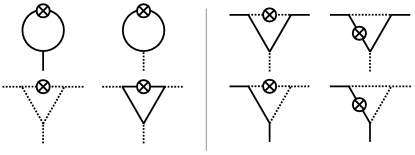
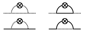
For the anomalous dimensions, encoded in the diagrams in Fig. 2, we find for both the flat and the sharp cutoffs
| (17) | ||||
| (18) |
Our conventions for the sharp-cutoff scheme follow those of Janssen:2012pq . For and with in the threshold functions this reduces to the anomalous dimensions given in Fei:2014yja , as it should (apart from a factor of 2 which is due to different conventions used in Fei:2014yja ).
For the effective potential we will employ two different ansätze. One suggestion is to treat the Hubbard-Stratonovich transformation similar to the one in many fermionic models and to simply consider an expansion of the dimensionless renormalized effective potential in the field, i.e.,
| (19) |
with a function that, for instance, can be expanded in a local potential approximation (LPA). Taking into account the wave function renormalizations or anomalous dimensions, we will refer to such a truncation scheme as LPA′. This truncation recovers the perturbative fixed-point solution from Ref. Fei:2014yja near , see the following section. In practice, we expand in a Taylor series to finite order, reading
| (20) |
where , and defines the order of the LPA, i.e., LPA. In the limit of we will also study the global properties of without expanding in the field, see Sec. VI.
III Extending the fixed point from to
We discuss the connection between the FRG and the -expansion scheme to show that both approaches coincide in the perturbative limit. This allows us to relate our results to the fixed-point solutions identified in Ref. Fei:2014yja . We will then study these results in detail within the FRG approach by evaluating the fixed-point properties directly in including nonperturbative effects, such as threshold terms in the loop integrals.
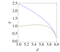
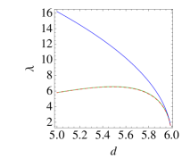
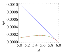
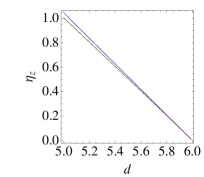
In the first order of the expansion the fixed-point solutions by Fei et al. Fei:2014yja appear at large . To be explicit, we compare the FRG and the -expansion results for ; however, the agreement we find does not depend on the specific choice of . For and to leading order in the results from the FRG and the expansion agree perfectly, as expected, cf. Fig. 3. Here, we have worked with the optimized regulator function as this is expected, at least for simple scalar models, to yield the best estimates for the critical exponents litim ; litim01 ; Pawlowski:2005xe ; Pawlowski:2015mlf . For the differences between the two approaches become sizable, which can be attributed to threshold corrections that contribute to the FRG functions. For better comparison, we also list the values for the couplings and the anomalous dimensions in and for the FRG and the expansion in Tab. 1. Within the FRG, we also show the values from two different truncation schemes (LPA3′ and LPA6′) to display the formidable convergence of the polynomial expansion in the field. For clarity, we display only the stable one of the two fixed points that appear in the expansion for , i.e. the one with the lowest number of RG relevant directions. The other, unstable fixed point which features an additional relevant direction is also found in our FRG approach and coincides with the unstable fixed point from expansion in the limit .
| approximation | |||||
|---|---|---|---|---|---|
| exp | 5.9 | 0.7801 | 5.1215 | 0.00010223 | 0.10444 |
| FRG LPA3′ | 5.9 | 0.7089 | 4.4708 | 0.00008289 | 0.10327 |
| FRG LPA6′ | 5.9 | 0.7089 | 4.4956 | 0.00008288 | 0.10329 |
| exp | 5 | 2.4670 | 16.1957 | 0.00102233 | 1.04436 |
| FRG LPA3′ | 5 | 0.9664 | 5.7938 | 0.00011043 | 1.00338 |
| FRG LPA6′ | 5 | 0.9664 | 5.7993 | 0.00011040 | 1.00338 |
IV Critical from the FRG
In the expansion the stable fixed point was found to exist only above a certain critical , with (beyond leading order) depending on the dimension . To leading order the result is independent of and one finds . As has been emphasized, e.g., in Fei:2014xta , it is highly desirable to use a nonperturbative method to obtain another estimate of beyond the expansion. We now compute within the truncation Eq. (5) with Eq. (19) of the functional renormalization group.
| approximation | |||||
|---|---|---|---|---|---|
| FRG LPA3′ | 1 | 70.686 | 346.221 | 0.00899 | 1.8108 |
| FRG LPA4′ | 1 | 70.632 | 347.484 | 0.00897 | 1.8096 |
| FRG LPA5′ | 1 | 70.622 | 350.745 | 0.00895 | 1.8097 |
| FRG LPA6′ | 1 | 70.622 | 350.777 | 0.00895 | 1.8097 |
| FRG LPA3′ | 2 | 46.411 | 231.184 | 0.01184 | 1.6921 |
| FRG LPA4′ | 2 | 46.342 | 233.323 | 0.01175 | 1.6898 |
| FRG LPA5′ | 2 | 46.336 | 236.466 | 0.01171 | 1.6903 |
| FRG LPA6′ | 2 | 46.334 | 236.541 | 0.01170 | 1.6902 |
| FRG LPA3′ | 10 | 16.802 | 90.398 | 0.01013 | 1.3474 |
| FRG LPA4′ | 10 | 16.783 | 93.060 | 0.00993 | 1.3464 |
| FRG LPA5′ | 10 | 16.787 | 94.725 | 0.00988 | 1.3477 |
| FRG LPA6′ | 10 | 16.786 | 94.870 | 0.00987 | 1.3477 |
In particular, we are interested in determining whether a minimal value of , below which the fixed point ceases to be real, exists within the FRG setting. As is obvious from Fig. 3, our results are close to those of the leading-order expansion for . Accordingly, our numerical evaluation indeed yields a critical value of , at which the stable fixed point merges with the unstable fixed point, and both disappear into the complex plane. For we get , while for we already find . Towards lower dimensionality, the critical value decreases, and we find in and in , cf. Fig. 4, in qualitative agreement with the -expansion results.
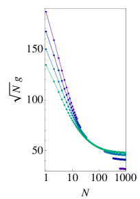
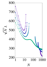
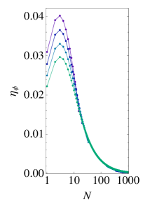
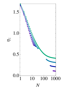
As a difference to the expansion, we find that the fixed point reappears on the real axis for lower values of , see Fig. 4. Near and below , there are two “islands” on the axis on which the fixed point is real. Below some noninteger critical dimension , we find that these two islands merge, and the fixed point exists at real values of the couplings for all , see Fig. 5.
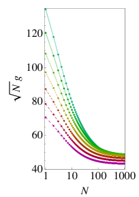
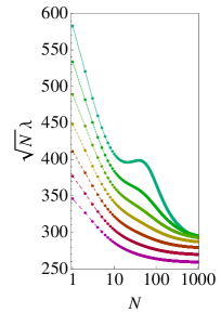
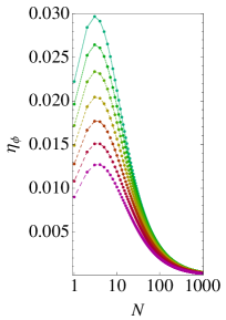
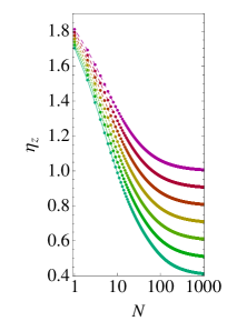
Within our approximation we obtain numerically. Our results thus suggest that a critical value of does not exist in the physical situation of . A summary of these findings is shown in Fig. 6 and the convergence of the results within the LPA′ is exhibited in Tab. 2.
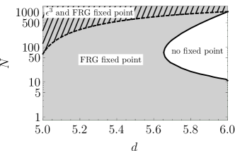
The existence of a second island for low and in which the fixed point reappears on the real axis is due to nonperturbative threshold effects of our FRG equations: In fact, we find that the fixed-point couplings in this “low- island” have values of , even when . This second island is therefore inaccessible by the perturbative expansion, even when is small. The reappearance of the fixed point at low near is in fact responsible for the occurrence of the noninteger critical dimension , and hence ultimately for the comparatively large quantitative disagreement between our FRG estimates and the values obtained from extrapolating the perturbative expansion to larger values of . While at present we cannot exclude the possiblity that the reappearance of the fixed point at low is an artifact of our truncation, we do not find any sign of breakdown of our approximation at low . A similar “low- island” has, in fact, recently been identified within the expansion of a related cubic theory in which the Hubbard-Stratonovich decoupling is made in the tensorial channel as opposed to the scalar channel Herbut:2015zqa . It is certainly tempting to identify these small- fixed points with our low- island. However, understanding the relation between the fixed points in the tensorial and scalar cubic models requires to overcome the ambiguity in the different Hubbard-Stratonovich decouplings of the interaction (so-called Fierz or mean-field ambiguity) Jaeckel:2002rm . Within the FRG, this would be possible by means of dynamical bosonization Gies:2001nw ; Pawlowski:2005xe ; Floerchinger:2009uf . This is left for future work.
The existence of a noninteger critical dimension below which the fixed point exists for all is in fact requisite to the conjecture that the fixed point of the cubic scalar theory in represents the analytic continuation of the Wilson-Fisher fixed point towards Fei:2014yja , as well as to the case where the universality class is embedded in that of our model, see Sec. V. In the Wilson-Fisher fixed point can be accessed by the expansion of a pure theory and hence is guaranteed to exist (though at negative quartic coupling) for all values of as long as is small. If the fixed point of our cubic model defines the cubic universality class in one therefore expects already on general grounds that there exists a critical dimension below which no merging and annihilation of fixed points occurs, with . The main question is only whether is above or below the physical dimension. Within our approximation we find and thus above . It should in principle be possible to test this scenario with standard Monte Carlo simulations. We conjecture that such simulations should display universal critical behavior governed by our stable fixed point for any value of in . We should emphasize, however, that it is unclear at present, whether a lattice formulation (with positive measure) exists, which allows to demonstrate the existence of our fixed point and assess its properties. We further discuss this problem in the concluding section.
Overall, the situation appears to be similar to the issue of the fixed-point structure of the three-dimensional Abelian Higgs model coleman1973 ; halperin1974 ; dasgupta1981 ; kolnberger1990 ; Bergerhoff:1995zm ; bergerhoff1996 ; herbut1996 ; herbut1997 ; Freire:2000sx : Within the expansion in dimensions, one finds a critical number of complex scalars below which a real and stable fixed point ceases to exist, with to leading order in the expansion coleman1973 ; halperin1974 . However, already the next-to-leading order term drastically reduces the estimate when extrapolated to kolnberger1990 ; herbut1997 . It has therefore been speculated that the standard expansion may be inapplicable to the physically relevant situation in , forcing one to go back to alternative approximations herbut1997 . The perturbative RG analysis in fixed herbut1996 , in agreement with earlier functional RG studies bergerhoff1996 , predicted that a stable and real fixed point may in fact continue to exist all the way down to . This scenario is also consistent with the data from lattice Monte Carlo simulations dasgupta1981 . It is therefore nowadays believed that in fact in , the lowest-order -expansion result notwithstanding herbut2007 .
V Comparison of universality classes
A universality class is characterized by universal scaling exponents. These include the anomalous dimensions of the fields, as well as the exponents that characterize the linearized RG flow of the essential couplings around a fixed point. Within a RG scheme that includes beta functions for the masses, all critical exponents can be obtained by diagonalizing the stability matrix in the vicinity of the fixed point. Specifically, denoting the set of all dimensionless couplings, including the masses, by , with fixed-point values , the stability matrix is given by
| (21) |
The critical exponents are defined as the eigenvalues of this matrix, multiplied by a negative sign,
| (22) |
In the vicinity of the Gaussian fixed point, the critical exponents agree exactly with the canonical dimensions of the couplings, whereas residual interactions result in additional contributions near an interacting fixed point. While beta functions of dimensionful couplings are non-universal, i.e., scheme-dependent, the critical exponents are scheme-independent. Thus the set of critical exponents is determined uniquely by the symmetries, dimensionality and degrees of freedom of a system.333Exceptions to this general rule have been discussed in Ref. Gehring:2015vja .
We will explicitly compare the critical exponents for the pure quartic model (analytically continued to ) with those of the cubic model specified in Eq. (1), in order to explore whether the universality classes agree. If they do not, then the pure model and the model that we consider here are actually inequivalant on the quantum level.
V.1 Analytic continuation of the Wilson-Fisher fixed point to
In the large- limit, solutions of the flow equation for the effective potential within the original quartic formulation are available Litim:1995ex ; Tetradis:1995br ; Mati:2016wjn , and yield Mati:2016wjn
| (23) |
in agreement with the simple analytic continuation of the result in ZinnJustin:1998cp . Similarly, the second-largest critical exponent of the large- fixed point is determined by
| (24) |
again continuing the result from Ref. ZinnJustin:1998cp towards . The Wilson-Fisher fixed point in thus has two relevant directions (), in contrast to the case of . The additional relevant direction is associated with the quartic coupling, which has canonical scaling dimension , and is therefore perturbatively irrelevant at the Gaussian fixed point. Thus the Gaussian fixed point is IR attractive in the quartic coupling. Accordingly a non-Gaussian fixed point will be UV attractive, i.e., IR relevant in that coupling. The other relevant direction is associated with the mass operator, and has canonical dimension independent of .
V.2 Universality class of the cubic model
For the model defined in Eq. (1) with the Hubbard-Stratonovich field we find the anomalous dimensions in the limit :
| (25) |
cf. Figs. 4, 5 and Sec. VI. The scaling dimensions for the fields and are thus
| (26) | |||||
| (27) |
in agreement with Ref. Fei:2014yja .
The beta functions for the two mass parameters in the simplest truncation specified by Eq. (6) in LPA2′, i.e., , read
| (28) | ||||
| (29) |
Further, the beta function for is
| (30) |
To obtain all critical exponents, it is crucial to consider also the renormalization of the operator linear in , i.e., the function for :
| (31) |
Including the expressions for the anomalous dimensions, Eq. (17) and (18), we find the interacting fixed point, which, e.g., in the case of , lies at
| (32) |
Inserting these fixed-point values in the expression for the stability matrix yields the critical exponents , and and . The result for and can be elucidated by the following argument: As the interacting fixed point that we consider emanates from the Gaussian fixed point in , we can assume that the critical exponents correspond to scaling dimensions of the couplings and at the fixed point. For these, the following equations hold:
| (33) | ||||
| (34) |
where we have inserted and , which holds in the large- limit. This argument also motivates this particular value for : The “composite” field must scale in that particular way, in order to reproduce scaling exponents from the pure quartic model. Our explicit results for for and approach the values in Eq. (33) and (34) very closely. This confirms that our reasoning does indeed explain the observed critical exponents: Essentially, the scaling at the interacting fixed point is the canonical scaling, shifted by the anomalous dimension for the field. The largest critical exponent can be understood as the anomalous scaling of the operator present in Eq. (6), which has scaling dimension . The explicit result in already highlights the existence of three relevant directions, i.e., positive critical exponents, in contrast to only two for the pure quartic model. This is true in any dimension , cf. Tab. 3, where we also include the self-interaction of the field (LPA3’). There, we use a notation in which the largest critical exponent, , is related to by . The second-largest critical exponent is denoted . The third-largest critical exponent is related to by .
We have plotted the critical exponents for various dimensions as a function of in Fig. 7. At large this confirms the expected behavior, where , and .
| 5.9 | 2000 | 0.256 | -1.9 | 0.257 | -1.904 | 2.002 |
|---|---|---|---|---|---|---|
| 5.8 | 2000 | 0.263 | -1.8 | 0.263 | -1.805 | 2.002 |
| 5.7 | 2000 | 0.270 | -1.7 | 0.270 | -1.705 | 2.003 |
| 5.6 | 2000 | 0.278 | -1.6 | 0.278 | -1.604 | 2.003 |
| 5.5 | 2000 | 0.286 | -1.5 | 0.286 | -1.504 | 2.003 |
| 5.4 | 2000 | 0.294 | -1.4 | 0.294 | -1.403 | 2.003 |
| 5.3 | 2000 | 0.303 | -1.3 | 0.303 | -1.302 | 2.002 |
| 5.2 | 2000 | 0.313 | -1.2 | 0.313 | -1.202 | 2.002 |
| 5.1 | 2000 | 0.326 | -1.1 | 0.323 | -1.101 | 2.002 |
| 5.0 | 2000 | 0.333 | -1.0 | 0.334 | -1.003 | 2.002 |
| 4.9 | 2000 | 0.345 | -0.9 | 0.345 | -0.901 | 2.001 |
| 4.8 | 2000 | 0.357 | -0.8 | 0.357 | -0.800 | 2.001 |
| 4.7 | 2000 | 0.370 | -0.7 | 0.371 | -0.700 | 2.001 |
| 4.6 | 2000 | 0.385 | -0.6 | 0.385 | -0.600 | 2.001 |
| 4.5 | 2000 | 0.400 | -0.5 | 0.400 | -0.500 | 2.001 |
| 4.4 | 2000 | 0.417 | -0.4 | 0.417 | -0.400 | 2.001 |
| 4.3 | 2000 | 0.435 | -0.3 | 0.435 | -0.300 | 2.000 |
| 4.2 | 2000 | 0.455 | -0.2 | 0.455 | -0.200 | 2.000 |
| 4.1 | 2000 | 0.476 | -0.1 | 0.476 | -0.100 | 2.000 |

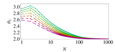
As discussed in Ref. Fei:2014yja , the operators and will feature couplings with scaling dimension at large . We are able to confirm this behavior within our approach, for instance at , where at and at .
The excellent agreement of the critical exponents and between the quartic model and the cubic model shows that the corresponding fixed points define related universality classes. Note that it is crucial to include the linear term into the flowing action to obtain a critical exponent that agrees with from the pure quartic model. On the other hand, there is an additional relevant direction in the cubic model, which is related to the mass-parameter of , cf. Eq. (34). The universality class of the quartic model is thus embedded into that of the cubic model: After tuning the third relevant direction, the remaining tuning that is required in order to reach the fixed point in the IR is exactly the same in both models. Towards the UV, there is a third attractive direction of the fixed point, i.e., the critical hypersurface is three-dimensional. A similar behavior occurs in another class of models which contain multiple scalar fields: Coupling an vector and an vector in results in a variety of fixed points, one of which is the so-called isotropic fixed point (IFP), at which the symmetry is enhanced to an symmetry herbut2007 . Thus, the critical exponents of the simple model can be recovered from the IFP. On the other hand, it features (at least) one additional relevant direction – again, the simpler universality class is embedded in the universality class of the model with additional fields Eichhorn:2013zza . The same structure can be observed in models with even more different sectors coupled to each other: The simplest universality class is amended by additional relevant directions, at least one for each additional direction that is added in field space Eichhorn:2014asa ; Eichhorn:2015woa .
VI Stability of the potential at large in
At large , a consistent truncation that is sufficient to investigate the stability of the potential is given by Eq. (19), i.e., , where no higher-order terms in the invariant appear. Here, we will argue that this truncation captures all contributions to the effective potential at leading order in : Additional interactions are either generated at subleading order in or feed back into the fixed-point equations for at subleading order in . Essentially, our argument relies on the fact that only loops which do not contain internal propagators contribute at leading order in . The only loops satisfying this requirement – given the truncation with the vertices from Eq. (19) – are those which generate pure self-interactions, i.e., loops that do not have external lines: A loop with external legs necessarily has to be constructed with the vertex which forces the line to be an internal line and consequently produces a diagram subleading in . Thus the “dangerous” interactions are the self-interactions in , as these are generated at leading order in and can couple back into the fixed-point equation for . For instance, momentum-dependent self-interactions, of the form , are generated from the -vertex by a closed -loop, which contributes at leading order in . However, just as in the case for the pure quartic model, the back-coupling of this term into the fixed-point equation for is given by a closed -loop, which is subleading in Morris:1997xj . Thus, it is self-consistent to neglect (momentum-dependent) self-interactions in our analysis of the stability of the potential at leading order in . Note that our argument relies on the analyticity of the potential, i.e., a diagrammatic expansion.
From now on, we will use the sharp cutoff exclusively, for reasons of computational simplicity. As we will see, it allows us to find an explicit solution to the flow equation for the effective potential that is well-defined at all values of the field . In the large- limit all diagrams with an internal propagator are suppressed, thus the flow equation for the effective potential becomes, using Eqs. (9) and (19),
| (35) |
and the flow of the mass of the field reduces to
| (36) |
From this we infer that any fixed point should have , since Eq (18) becomes for large :
| (37) |
As can be seen from Fig. 1, all explicit contributions to are also suppressed by . Accordingly, Eq. (30) reduces to the simple form
| (38) |
from which the fixed-point requirement again shows that
| (39) |
The fixed-point value for can be obtained from Eq. (17), which for large reduces to , and thus .
The flow of the original model with quartic coupling can in fact be recovered from Eqs. (38) and (35):
| (40) |
which is the large- one-loop beta function for the standard theory herbut2007 upon identification , which is precisely the relation expected from the Hubbard Stratonovich transformation.
With the known fixed-point values for and we can solve Eq. (35) for the fixed-point potential with :
| (41) |
with arbitrary constant . The form of the potential is plotted for two values of in Fig. 8. The potential has the following behavior for small :
| (42) |
while for large we find:
| (43) |
with being the Heaviside step function. As discussed, e.g., in Morris:1994ki ; Morris:1994jc ; Morris:1997km , the solution at large values of is given by the dimensional scaling (including the anomalous dimension) which in our case gives at positive . If the fixed-point potential is real, the corresponding expression for negative should be . Focussing on the case , the large- scaling is produced by the same terms that admit a Taylor expansion at low , i.e., the large -scaling provides a boundary condition for the analytic solution. This case is clearly realized for , and provides . On the other hand, we find . This is a special case of the general scaling ansatz, and shows that for our case.
Note a major difference of our model to the case of, e.g., the Wilson-Fisher fixed point with one field species: In the latter case, the solution to the homogenous equation, i.e., the one determined by dimensional scaling, only holds at large field values, as the threshold function depends on the derivatives of the potential. In that case, the right-hand side of the Wetterich equation contains a term . Only in the asymptotic large-field regime can this term be neglected, and the dimensional scaling ansatz therefore only describes the behavior of the solution at large fields, but not everywhere. In contrast, our case features a threshold function that is independent of the potential , as the fluctuating modes dominating at large are not those of the -field. Thus, the solution to the homogenous equation, can be added to that of the inhomogeneous equation at all field values and can be chosen freely. It is only restricted by analyticity-considerations, but any value of provides a solution to the fixed-point equation. We can now ask whether this property will persist at finite . In that case, the -fluctuations will enter the right-hand-side of the equation and an additional term will appear. Then, the situation will be analogous to that of the Wilson-Fisher fixed point with one field species: The dimensional scaling ansatz will only hold asymptotically, at large field values. It will not be possible to add a term to the solution. Thus, the case of finite will restrict the viable solutions to . Demanding a continuous large- limit thus suggests to set everywhere.
If we insist on the large- fixed-point potential being analytic in , we must choose . In this case the potential is unbounded from below. On the other hand, if we allow a small non-analyticity, e.g., with , the fixed-point potential becomes completely stable (dashed line in Fig. 8). Within perturbation theory, a non-analytic contribution to the microscopic action would prohibit a straightforward interpretation in terms of Feynman diagrams. Even beyond perturbation theory, one would usually demand a theory space that can be spanned in terms of functions that admit a Taylor expansion. Admitting further non-analytic functions to extend the basis in theory space presumably could result in problems with predictivity, as each of these functions comes with a coupling that could become relevant. As a simple example, consider all functions of the form , with . These come with couplings of increasing canonical mass dimension, and therefore result in an infinite number of free parameters, if the theory is considered in the vicinity of the Gaussian fixed point. For these reasons, we conclude that seems to be the only viable choice in a perturbative context444On the other hand, explicit examples are known where fixed-point potentials exhibit nonanalyticities, which are nonperturbative phenomena, see, e.g., David:1984we ..
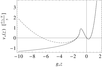
We thus conclude that the potential is not stable in the large limit in the direction, at least if we insist on analyticity. Our results indicate that the situation for the model with an additional scalar coupled through a cubic interaction is analogous to that for the pure quartic model Percacci:2014tfa : There, also no analytic fixed-point solution that features a stable fixed-point potential exists at large . As a next step, we will investigate the direction, and also consider the situation at finite .
VII Potential stability at finite
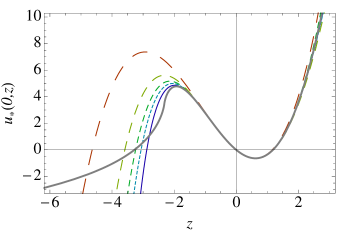
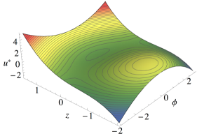
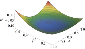
We are interested in the properties of the potential in the vicinity of , in the two-dimensional field space spanned by and . This can efficiently be captured by considering a two-dimensional Taylor expansion in the bosonic fields and
| (44) |
Then, we have , and , cf. Eq. (6).
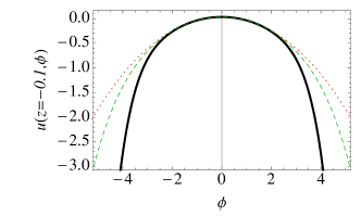
To highlight that such an expansion already works very well on a quantitative level at low orders of the expansion in the vicinity of the local minimum, we compare the results in the LPA′ at different orders to the full solution at large , cf. Fig. 9. On the other hand, just as one should expect within a local expansion, the global properties are captured less well; in particular the LPA′ overestimates the drop of the potential at negative .
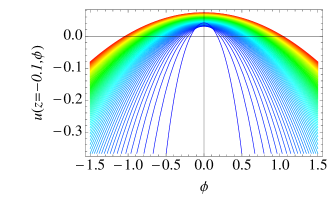
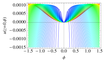
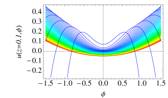
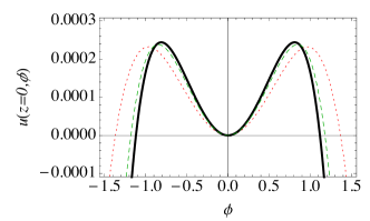
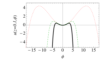
We now use the two-field expansion, Eq. (44), to investigate the fixed point at finite . We observe the existence of a local minimum in the two-dimensional space spanned by and , cf. Fig. 10. In the direction, the local minimum is generated by a positive mass term, . All higher-order terms in the direction are negative, for . This results in an instability of the potential towards larger absolute values of . While the expansion of a globally stable potential can feature negative coefficients at some order in the fields, the coefficients typically alternate in sign in the case of a globally stable potential. In contrast, we observe that all coefficients for are negative, suggesting the onset of instability.
As a next step, we explore whether quantum fluctuations of , which become more important at smaller feature signatures of a stabilization mechanism for the fixed-point potential: In fact, our result indicates the opposite behavior as expected from our analysis of the constant in Eq. (41): Towards negative , we observe an unstable potential. Moreover, the lower the value of the faster the onset of instability towards large , see Fig. 11. As both mass terms, and , stay positive at the fixed point and a local minimum always exists at . Our results however do not indicate a stabilization of that local minimum, as all higher-order couplings stay negative, see Fig. 12 for a study of the convergence within the LPA′. In the region where the LPA′ converges around the local minimum, our results indicate that the minimum cannot be the global one. Let us emphasize that a local expansion of the flow equation for the fixed-point potential cannot efficiently detect the formation of a second, global minimum. If such a second minimum existed, and the potential were bounded from below, the situation would correspond to metastability. To explore this potential possibility, global-solution methods must be applied, such as, e.g., those of Ref. Borchardt:2015rxa . With the local expansion employed here we can only exclude that the local minimum close to the origin appears not to be a global minimum as our local expansion captures the onset of instability.
The fixed-point potential is unstable in the direction at large , unless we allow for the existence of non-analytic terms which we conjecture to also violate continuity of the solution in , and we do not detect a stabilization mechanism at finite . We thus conclude that our results suggest that the fixed-point potential is unstable, at least in the vicinity of the origin.
VIII Conclusions
We have explored an symmetric model with an vector coupled to an additional composite field via a cubic interaction. It has recently been proposed that this model features an UV fixed point in dimensions Fei:2014yja , thus representing another candidate for an asymptotically safe quantum field theory. Within a one-loop and higher-order expansion in dimension , the fixed point was found to lie at real values of the couplings only above a critical number of components of the vector field . The estimate for when extrapolated to the relevant case has been found to drastically depend on the order of the expansion. Thus, a central question is whether one can find an estimate for beyond the perturbative expansion. For our study, we have employed the functional renormalization group, which can capture the relevant physics in any dimension directly. In the vicinity of , our method reproduces the results for the fixed-point values and anomalous dimensions found within the expansion.
In the introduction, we have identified three central questions, which we have set out to answer.
-
1.
What is the true in five dimensions?
Following this fixed point to , we find that decreases rapidly, in qualitative but not quantitative agreement with the -expansion results. Within our approximation, we find that a stable and real fixed point exists all the way down to for all dimensions with , cf. Fig. 6. In this context, stability refers to the number of relevant directions, which we find to be three, see below. Our results thus suggest that there exists no for all in .
-
2.
Does the classical equivalence of the cubic theory defined by Eq. (1) and the original quartic model continue on the quantum level?
We have explored the universal scaling exponents of the cubic model, explicitly comparing with those of the pure universality class at large . We find that two of the relevant critical exponents precisely agree, while the cubic model features an additional RG relevant direction with positive critical exponent. Thus, the universality class of the pure quartic model is actually embedded in that of the cubic model. Our results imply that the models are not fully equivalent, unless one already restricts some of the couplings to lie on the critical hypersurface of the fixed point. This suggests that physically, the additional field is in fact a new, independent degree of freedom in the model, instead of simply capturing momentum-dependent interactions in the pure model in a more efficient way.
-
3.
Does the cubic model feature a stable fixed-point potential?
We have explored the global properties of the fixed-point potential at large , which turned out to be unstable towards negative , unless nonanalytic terms are allowed in the fixed-point action. This is similar to the results of the analysis of the model within the original quartic formulation Percacci:2014tfa .
In order to address the situation at finite , we have evaluated the fixed-point potential in the two-dimensional field space spanned by and . While we uncover the existence of a local minimum, it only exists due to a positive mass term for , while all higher-order couplings in are negative. This suggests the onset of instability for larger values of . Moreover, our local expansion features an instability towards large negative , as is already implied by the analytic solution for large . We should emphasize that our finite- study, based on a local expansion of the potential, cannot firmly exclude the possibility that quantum fluctuations generate a second minimum at larger field values. This could result in a potential that is globally bounded from below, and would imply that the minimum that we have investigated here is in fact metastable. To address this question, global methods such as those in Borchardt:2015rxa should be employed. This is left for a future study. Here, we can only conclude that quantum fluctuations do not appear to stabilize the local minimum, but in fact trigger a faster onset of its instability towards lower .
The fixed point of the cubic model hence appears to suffer from the same deficiency as the Wilson-Fisher fixed point of the original quartic model in , at least at large and as long as one insists on an analytic fixed-point potential. This raises the question whether it may at all be possible, at least in principle, to find an explicit (e.g., lattice) construction with positive measure whose continuum limit realizes our fixed point. The known lattice models Aizenman:1981du ; Frohlich:1982tw ; Wolff:2009ke exhibit (in agreement with the perturbative expectation Wilson:1973jj ) trivial critical behavior, governed by the noninteracting Gaussian fixed point. It is not clear whether a lattice study can assess the nontrivial fixed point of our cubic theory, as it would require to overcome the notorious difficulties that arise through the nonanalyticities of the fixed-point potential.
In summary, we have found an interacting fixed point of the cubic model which exists for all in . The universality class it defines includes the standard universality class (analytically continued to ), but features an additional RG relevant direction. On the quantum level, the cubic model hence is not fully equivalent to the original quartic model. Our study indicates that no stable analytic fixed-point potential can be found, questioning the realization of the fixed point from underlying a well-defined quantum field theory.
Acknowledgements.
We thank Holger Gies and Daniel F. Litim for helpful discussions and comments on this manuscript. We also thank Igor Boettcher and Jan M. Pawlowski for discussions and Igor F. Herbut for collaboration on an earlier related project. M.M.S. thanks the Imperial College for hospitality. M.M.S. is supported by Grant No. ERC-AdG-290623 and DFG Grant No. SCHE 1855/1-1. L.J. acknowledges support by the DFG under Grant No. SFB1143. The work of A.E. is supported by an Imperial College Junior Research Fellowship.References
- (1) L. Fei, S. Giombi and I. R. Klebanov, Phys. Rev. D 90, 025018 (2014) [arXiv:1404.1094 [hep-th]].
- (2) L. Fei, S. Giombi, I. R. Klebanov and G. Tarnopolsky, Phys. Rev. D 91, 045011 (2015) [arXiv:1411.1099 [hep-th]].
- (3) S. Weinberg, in General Relativity, edited by S. Hawking and W. Israel (Cambridge University Press, Cambridge, England, 1979), pp. 790-831.
- (4) H. Gies, S. Rechenberger, M. M. Scherer and L. Zambelli, Eur. Phys. J. C 73 (2013) 2652 [arXiv:1306.6508 [hep-th]].
- (5) D. F. Litim and F. Sannino, JHEP 1412, 178 (2014) [arXiv:1406.2337 [hep-th]].
- (6) M. Reuter, Phys. Rev. D 57, 971 (1998) [hep-th/9605030].
- (7) A. Codello, R. Percacci and C. Rahmede, Annals Phys. 324, 414 (2009) [arXiv:0805.2909 [hep-th]].
- (8) D. Benedetti, P. F. Machado and F. Saueressig, Mod. Phys. Lett. A 24, 2233 (2009) [arXiv:0901.2984 [hep-th]].
- (9) K. Falls, D. F. Litim, K. Nikolakopoulos and C. Rahmede, arXiv:1301.4191 [hep-th].
- (10) D. Becker and M. Reuter, Annals Phys. 350, 225 (2014) [arXiv:1404.4537 [hep-th]].
- (11) P. Donà, A. Eichhorn and R. Percacci, Phys. Rev. D 89, 084035 (2014) [arXiv:1311.2898 [hep-th]].
- (12) E. S. Fradkin and M. A. Vasiliev, Phys. Lett. B 189, 89 (1987).
- (13) M. A. Vasiliev, Phys. Lett. B 243, 378 (1990).
- (14) M. A. Vasiliev, Phys. Lett. B 285, 225 (1992).
- (15) M. A. Vasiliev, Int. J. Mod. Phys. D 5, 763 (1996) [hep-th/9611024].
- (16) M. A. Vasiliev, In The many faces of the superworld, edited by M. A. Shifman (World Scientific, Singapore, 2000), pp. 33-610 [hep-th/9910096].
- (17) M. A. Vasiliev, Phys. Lett. B 567, 139 (2003) [hep-th/0304049].
- (18) I. R. Klebanov and A. M. Polyakov, Phys. Lett. B 550, 213 (2002) [hep-th/0210114].
- (19) S. Giombi, I. R. Klebanov and B. R. Safdi, Phys. Rev. D 89, 084004 (2014) [arXiv:1401.0825 [hep-th]].
- (20) H. Gies and M. M. Scherer, Eur. Phys. J. C 66, 387 (2010) [arXiv:0901.2459 [hep-th]].
- (21) H. Gies, S. Rechenberger and M. M. Scherer, Eur. Phys. J. C 66 (2010) 403 [arXiv:0907.0327 [hep-th]].
- (22) M. M. Scherer, H. Gies and S. Rechenberger, Acta Phys. Polon. Supp. 2, 541 (2009) [arXiv:0910.0395 [hep-th]].
- (23) G. P. Vacca and L. Zambelli, Phys. Rev. D 91, 125003 (2015) [arXiv:1503.09136 [hep-th]].
- (24) J. A. Gracey, Phys. Rev. D 92, 025012 (2015) [arXiv:1506.03357 [hep-th]].
- (25) Y. Nakayama and T. Ohtsuki, Phys. Lett. B 734, 193 (2014) [arXiv:1404.5201 [hep-th]].
- (26) S. M. Chester, S. S. Pufu and R. Yacoby, Phys. Rev. D 91, 086014 (2015) [arXiv:1412.7746 [hep-th]].
- (27) J. B. Bae and S. J. Rey, arXiv:1412.6549 [hep-th].
- (28) I. F. Herbut and L. Janssen, Phys. Rev. D 93, 085005 (2016) [arXiv:1510.05691 [hep-th]].
- (29) S. R. Coleman and E. J. Weinberg, Phys. Rev. D 7, 1888 (1973).
- (30) B. I. Halperin, T. C. Lubensky and S. K. Ma, Phys. Rev. Lett. 32, 292 (1974).
- (31) S. Kolnberger and R. Folk, Phys. Rev. B 41, 4083 (1990).
- (32) B. Bergerhoff, D. Litim, S. Lola and C. Wetterich, Int. J. Mod. Phys. A 11, 4273 (1996) [cond-mat/9502039].
- (33) I. F. Herbut and Z. Tesanovic, Phys. Rev. Lett. 78, 980 (1997) [cond-mat/9605185].
- (34) I. F. Herbut and Z. Tesanovic, Phys. Rev. Lett. 76, 4588 (1996).
- (35) B. Bergerhoff, F. Freire, D. F. Litim, S. Lola, and C. Wetterich, Phys. Rev. B 53, 5734 (1996).
- (36) C. Dasgupta and B. I. Halperin, Phys. Rev. Lett. 47, 1556 (1981); J. Bartholomew, Phys. Rev. B 28, 5378(R) (1983); S. Mo, J. Hove, and A. Sudbo, Phys. Rev. B 65, 104501 (2002).
- (37) F. Freire and D. F. Litim, Phys. Rev. D 64, 045014 (2001) [hep-ph/0002153].
- (38) I. Herbut, A modern approach to critical phenomena, Cambridge University Press, Cambridge, 2007.
- (39) J. Berges, N. Tetradis and C. Wetterich, Phys. Rept. 363 (2002) 223 [hep-ph/0005122].
- (40) R. Percacci and G. P. Vacca, Phys. Rev. D 90, 107702 (2014) [arXiv:1405.6622 [hep-th]].
- (41) C. Wetterich, Phys. Lett. B 301, 90 (1993).
- (42) S. M. Christensen and M. J. Duff, Phys. Lett. B 79, 213 (1978); R. Gastmans, R. Kallosh and C. Truffin, Nucl. Phys. B 133, 417 (1978); H. Kawai and M. Ninomiya, Nucl. Phys. B 336, 115 (1990); H. Kawai, Y. Kitazawa and M. Ninomiya, Nucl. Phys. B 393, 280 (1993) [hep-th/9206081]; ibid. 467, 313 (1996) [hep-th/9511217].
- (43) T. R. Morris, Int. J. Mod. Phys. A 9, 2411 (1994) [hep-ph/9308265].
- (44) U. Ellwanger, Z. Phys. C 62, 503 (1994) [hep-ph/9308260].
- (45) J. Polonyi, Central Eur. J. Phys. 1, 1 (2003) [hep-th/0110026].
- (46) J. M. Pawlowski, Annals Phys. 322 (2007) 2831 [arXiv:hep-th/0512261].
- (47) H. Gies, Lect. Notes Phys. 852, 287 (2012) [arXiv:hep-ph/0611146].
- (48) B. Delamotte, Lect. Notes Phys. 852, 49 (2012) [cond-mat/0702365].
- (49) O. J. Rosten, arXiv:1003.1366 [hep-th].
- (50) J. Braun, J. Phys. G 39, 033001 (2012) [arXiv:1108.4449 [hep-ph]].
- (51) W. Metzner et al., Rev. Mod. Phys. 84, 299 (2012).
- (52) D. F. Litim, Phys. Rev. D 64, 105007 (2001) [hep-th/0103195].
- (53) J. Braun, H. Gies, L. Janssen and D. Roscher, Phys. Rev. D 90, 036002 (2014) [arXiv:1404.1362 [hep-ph]].
- (54) M. Reuter and F. Saueressig, Phys. Rev. D 65, 065016 (2002) [hep-th/0110054].
- (55) L. Janssen and H. Gies, Phys. Rev. D 86, 105007 (2012) [arXiv:1208.3327 [hep-th]].
- (56) D. F. Litim, Phys. Lett. B 486, 92 (2000) [hep-th/0005245]; Int. J. Mod. Phys. A 16, 2081 (2001) [hep-th/0104221]; Nucl. Phys. B 631, 128 (2002) [hep-th/0203006].
- (57) J. M. Pawlowski, M. M. Scherer, R. Schmidt and S. J. Wetzel, arXiv:1512.03598 [hep-th].
- (58) J. Jaeckel and C. Wetterich, Phys. Rev. D 68, 025020 (2003) [hep-ph/0207094].
- (59) H. Gies and C. Wetterich, Phys. Rev. D 65, 065001 (2002) [hep-th/0107221].
- (60) S. Floerchinger and C. Wetterich, Phys. Lett. B 680, 371 (2009) [arXiv:0905.0915 [hep-th]].
- (61) F. Gehring, H. Gies and L. Janssen, Phys. Rev. D 92, 085046 (2015) [arXiv:1506.07570 [hep-th]].
- (62) P. Mati, arXiv:1601.00450 [hep-th].
- (63) D. Litim and N. Tetradis, hep-th/9501042.
- (64) N. Tetradis and D. F. Litim, Nucl. Phys. B 464, 492 (1996) [hep-th/9512073].
- (65) J. Zinn-Justin, hep-th/9810198.
- (66) A. Eichhorn, D. Mesterházy and M. M. Scherer, Phys. Rev. E 88, 042141 (2013) [arXiv:1306.2952 [cond-mat.stat-mech]].
- (67) A. Eichhorn, D. Mesterházy and M. M. Scherer, Phys. Rev. E 90, 052129 (2014) [arXiv:1407.7442 [cond-mat.stat-mech]].
- (68) A. Eichhorn, T. Helfer, D. Mesterházy and M. M. Scherer, Eur. Phys. J. C 76, 88 (2016) [arXiv:1510.04807 [cond-mat.stat-mech]].
- (69) T. R. Morris and M. D. Turner, Nucl. Phys. B 509, 637 (1998) [hep-th/9704202].
- (70) T. R. Morris, Phys. Lett. B 334, 355 (1994) [hep-th/9405190].
- (71) T. R. Morris, Phys. Lett. B 345, 139 (1995) [hep-th/9410141].
- (72) T. R. Morris, hep-th/9709100.
- (73) F. David, D. A. Kessler and H. Neuberger, Phys. Rev. Lett. 53, 2071 (1984).
- (74) J. Borchardt and B. Knorr, Phys. Rev. D 91, 105011 (2015) [arXiv:1502.07511 [hep-th]].
- (75) M. Aizenman, Phys. Rev. Lett. 47, 1 (1981).
- (76) J. Frohlich, Nucl. Phys. B 200, 281 (1982).
- (77) U. Wolff, Phys. Rev. D 79, 105002 (2009) [arXiv:0902.3100 [hep-lat]], and references therein.
- (78) K. G. Wilson and J. B. Kogut, Phys. Rept. 12, 75 (1974).
