On the weakly competitive case in a two-species chemotaxis model

Abstract

In this article we investigate a parabolic-parabolic-elliptic two-species chemotaxis system with weak competition and show global asymptotic stability of the coexistence steady state under a smallness condition on the chemotactic strengths, which seems more natural than the condition previously known.
For the proof we rely on the method of eventual comparison, which thereby is shown to be a useful tool even in the presence of chemotactic terms.
Keywords: chemotaxis; two-species; logistic source; Lotka-Volterra competition
Mathematics Subject Classification (2010): Primary: 35B40; Secondary: 35B51, 92C17, 92D40, 35A01, 35B35.

1 Introduction

The questions how different populations living in the same habitat interact with each other and with their surroundings are central to mathematical biology.

The competition for resources by two species (in contrast to, e.g., one being prey to the other) is often modeled by means of Lotka-Volterra type competition terms, i.e. with coupling coefficients $a_{1}>0$, $a_{2}>0$ in

$$u_{t}=u(1-u-a_{1}v),\qquad v_{t}=v(1-v-a_{2}u).$$

We refer to [15] for conditions for global stability of fixed points in such systems: If $a_{1}>0$ and $a_{2}>0$, for positive equilibria to be globally stable it is sufficient that they be locally stable.

Of course, spatial homogeneity is a highly idealized situation, and dependence of the population size on a spatial variable together with the effects of random motion of individuals has been incorporated into the model (see e.g. [32, Chapter 1.2] and references therein).

One way of even simplest lifeforms to react to their environment is chemotaxis, that is the tendency to move in the direction of higher concentrations of a signal substance. Inter alia, effects of chemotaxis on possible population size have been considered in [24].

Exploitation of chemotaxis for biotechnological purposes in mind and envisioning applications in e.g. agriculture (like nitrogen fixation or denitrification), or in mammalian intestinal microbial ecology, in [25] the authors compare species that undergo growth with different rates and diffusive versus diffusive plus chemotactic motion. They conclude: “Thus, chemotaxis can, when the response is sufficiently strong, overcome both disadvantages of inferior growth kinetics and random motility. […] At any rate, these results suggest that chemotactic responses might provide a useful means for controlling population dynamics in nonmixed systems. In particular, they provide a way to permit slowly growing populations to coexist with or outcompete faster growing species. Such a situation might be highly desirable in many environmental or biotechnological applications.” For the effectiveness of nutrient-taxis as advantageous dispersal strategy for populations in heterogeneous environments see e.g. [29, 8].

Chemotaxis terms in combination with several populations also appear in the context of the host-parasite interaction modelled and analyzed in [39] and [41], the food-chain model of [28], or the system in [5] that deals with the spread of an epidemic disease.

For one single species, chemotaxis is described by the celebrated model by Keller and Segel

$$u_{t} =\Delta u-\nabla\cdot(u\nabla v), \qquad\tau v_{t} =\Delta v-v+u,$$ (1.1)

which has been treated intensively over the last decades. We refer to the surveys [16, 17, 4].

Incorporating growth terms into this model, that is, adding $\kappa u-\mu u^{2}$ to the first equation in (1.1) (studied in [43, 50, 51, 23]), gives rise to colorful dynamics as witnessed in e.g. [38], emphasized by attractor results in [21, 33, 2, 34] or illustrated by recent results on transient growth phenomena in [52], [22].

One of the most straightforward generalizations of this model to the situation of several species is to consider two species (or two subpopulations of one species) that react to the same signalling substance they both produce, as occurring in the differentiation of cell-types during slime mold formation in populations of Dictyostelium discoideum, cf. e.g. [30, 45].

The pure two-species chemotaxis model without growth or competition effects has been introduced in [53] and in particular blow-up of solutions in finite time, known to occur in the single-species situation, has been investigated also for the several species model (see e.g. [18]), both as to the question of occurrence of blow-up versus global existence (see [6, 7, 11, 20, 10, 27]) and of qualitative features of the former, for example whether it occurs simultaneously ([14, 12]) in both species, or nonsimultaneously ([13]); for numerical observations pertaining to these models also confer [19]. Furthermore, the long term behaviour of globally existent solutions emanating from small initial data ([54, 26]) or for chemosensitivity functions capturing saturation effects ([36]) has been investigated.

A combination of the two mechanisms introduced so far (Lotka-Volterra type competition and Keller-Segel type chemotaxis) is examined in the two-species chemotaxis-competition model

$$\begin{cases}u_{t}=d_{1}\Delta u-\chi_{1}\nabla\cdot(u\nabla w)+\mu_{1}u(1-u-a_{1}v),&x\in\Omega,\ t>0,\\[2.84526pt] v_{t}=d_{2}\Delta v-\chi_{2}\nabla\cdot(v\nabla w)+\mu_{2}v(1-a_{2}u-v),&x\in\Omega,\ t>0,\\[2.84526pt] \tau w_{t}=d_{3}\Delta w+\alpha u+\beta v-\gamma w,&x\in\Omega,\ t>0,\\[2.84526pt] \nabla u\cdot\nu=\nabla v\cdot\nu=\nabla w\cdot\nu=0,&x\in\partial\Omega,\ t>0,\\[2.84526pt] u(x,0)=u_{0}(x),\;v(x,0)=v_{0}(x),\;w(x,0)=w_{0}(x),&x\in\Omega,\end{cases}$$ (1.2)

where $u$ and $v$ denote the population densities of two species undergoing chemotaxis in reaction to the signal having concentration $w$, posed in a bounded smooth domain $\Omega\subset\mathbb{R}^{n}$. Herein, the diffusion rates of species and signal are given by $d_{1},d_{2},d_{3}>0$, whereas $\mu_{i}>0,\chi_{i}\geq 0,a_{i}\geq 0$ ($i\in\{1,2\}$) are used to denote the strengths of chemotaxis, growth kinetics and competition for each species, whereas the size of $\alpha>0$, $\beta>0$ and $\gamma>0$ regulates the production of the signal by the first and second species and its decay, respectively. This model has first been considered in [44] for $\tau=0$, where it was shown for the weakly competitive case, i.e.

$$a_{1},a_{2}\in[0,1),$$ (1.3)

that solutions to (1.2) exist and converge to the coexistence steady state

$$(u_{*},v_{*},w_{*})=\left(\frac{1-a_{1}}{1-a_{1}a_{2}},\frac{1-a_{2}}{1-a_{1}a_{2}},\frac{2-a_{1}-a_{2}}{1-a_{1}a_{2}}\right),$$

provided that

$$2(\chi_{1}+\chi_{2})+a_{1}\mu_{2}<\mu_{1}\quad\text{and}\quad 2(\chi_{1}+\chi_{2})+a_{2}\mu_{1}<\mu_{2}.$$ (1.4)

Result and proof of [44] have successfully been extended to a setting of even more species in [48], the condition being analogous to (1.4).

This condition seems quite unnatural, because it is not automatically satisfied in the absence of chemotaxis ($\chi_{1}=\chi_{2}=0$) and it is the goal of the present paper to replace this condition by a smallness condition on $\frac{\chi_{i}}{\mu_{i}}$, $i\in\{1,2\}$ alone and to thus remove the additional condition on $a_{1}$, $a_{2}$, $\mu_{1}$, $\mu_{2}$ implicitly posed by (1.4):

Theorem 1.1.

Let $n\geq 1$ and $\Omega\subset\mathbb{R}^{n}$ be a bounded domain with smooth boundary. Let $\tau=0$ and $d_{1},d_{2},d_{3},\alpha,\beta,\gamma\in(0,\infty)$. Let $a_{1}$, $a_{2}$ fulfil (1.3) and let $\chi_{1}\geq 0$, $\chi_{2}\geq 0$ and $\mu_{1},\mu_{2}>0$ be such that $q_{1}:=\frac{\chi_{1}}{\mu_{1}}$, $q_{2}:=\frac{\chi_{2}}{\mu_{2}}$ satisfy the conditions:

$$q_{1}\in\big{[}0,\tfrac{d_{3}}{2\alpha}\big{)}\cap\big{[}0,\tfrac{a_{1}d_{3}}{\beta}\big{)},\quad q_{2}\in\big{[}0,\tfrac{d_{3}}{2\beta}\big{)}\cap\big{[}0,\tfrac{a_{2}d_{3}}{\alpha}\big{)},$$ (1.5)

$$a_{1}a_{2}d_{3}^{2}<(d_{3}-2\alpha q_{1})(d_{3}-2\beta q_{2}).$$ (1.6)

Then the following holds:

1. For all nonnegative functions $u_{0}$, $v_{0}\in C(\overline{\Omega})$ satisfying $u_{0}\not\equiv 0$, $v_{0}\not\equiv 0$, there exists a unique global-in-time classical solution $(u,v,w)\in\left(C^{0}(\overline{\Omega}\times[0,\infty))\cap C^{2,1}(\overline{\Omega}\times(0,\infty))\right)^{3}$ of (1.2) such that $u>0$, $v>0$ and $w>0$ in $\overline{\Omega}\times(0,\infty)$.

2. The unique global solution $(u,v,w)$ of (1.2) has the following asymptotic behaviour:

   $$u(t)\to u^{\ast},\quad v(t)\to v^{\ast},\quad w(t)\to\frac{\alpha u^{\ast}+\beta v^{\ast}}{\gamma}\quad\mbox{as}\ t\to\infty,$$

   uniformly in $\Omega$, where

   $$u^{\ast} =\frac{1-a_{1}}{1-a_{1}a_{2}},\quad\text{and}\quad v^{\ast}=\frac{1-a_{2}}{1-a_{1}a_{2}}.$$

We want to emphasize that (1.5) can indeed be viewed as a smallness condition on the relative chemotactic strength only and, in particular, satisfied in the chemotaxis-free case ($\chi_{1}=\chi_{2}=0$).

The case of partially strong competition ($a_{1}>1>a_{2}>0$) was considered in [40]. It was shown that solutions exist globally and satisfy $(u(t),v(t))\to(0,1)$ if $q_{1}\leq a_{1}$, $q_{2}<\frac{1}{2}$, $\alpha q_{1}+\max\{q_{2},\frac{a_{2}-a_{2}q_{2}}{1-2q_{2}},\frac{\alpha q_{2}-a_{2}q_{2}}{1-2q_{2}}\}<1$.

In the fully parabolic system ((1.2) with $\tau=1$), it was proven in [3] that for sufficiently large values of $\mu_{1}$, $\mu_{2}$ global classical solutions converge to the unique positive homogeneous equilibrium exponentially for $a_{1}>1>a_{2}>0$ (and with an algebraic rate if $a_{1}=1$ and $\mu_{2}$ is large), and moreover that there are global bounded classical solutions for $n\leq 2$ even if the parameters of the system are merely positive.

Furthermore, in spatially one-dimensional domains more insight into qualitative behaviour of the system has been obtained in [46] and [47], where global existence of solutions was shown as well as existence of nonconstant steady states by bifurcation analysis. The stability of the bifurcating solutions is investigated there, too, and a time-periodic solution has been found. Additionally, the findings have also been illustrated by numerical experiments ([47, Sec. 4]).

In [55], for different sensitivity functions satisfying $\chi_{i}(w)\leq\frac{K_{i}}{(1+\alpha_{i}w)^{k_{i}}}$ for some $k_{i}>1$, $i\in\{1,2\}$, global bounded classical solutions were proven to exist under the condition of $\chi,\mu,K$ being sufficiently small (where the meaning of ’sufficiently small’ depends on the initial mass).

In the competition-free case ($a_{1}=a_{2}=0$) for sensitivity functions generalizing $\frac{\chi_{i,0}}{(1+w)^{k}}$ ($k>1$), global existence and boundedness of solutions were obtained, together with a result on asymptotic stability of steady states. ([31])

A system where the chemoattractant is not a signal substance produced by the population itself but a nutrient which is consumed, (but which is otherwise similar), has been treated in [56, 49].

Let us finally mention that also (parabolic-elliptic) Keller-Segel type systems of two species and two chemicals have been studied where the signal for each species is produced by the other ([42]).

A parabolic-parabolic-ODE model with connections to chemotaxis-haptotaxis models (see e.g. [9]) has been treated in [37].

Cross-diffusive effects like those added to the present system by means of the chemotaxis term pose a serious threat to any monotonicity properties one would like to employ and usually should render comparison arguments useless. Nevertheless, in some situations closely related, comparison methods were employable, for example the proof of the result in [44] relies on comparison with solutions to a system of four coupled ODEs. (In fact, a system closely related to (1.2) was considered as example in [35], where comparison with solutions of ODE systems has been developed more systematically. However, there the essential coupling arising from the appearance of $u$ and $v$ as source terms for the third equation was not included.)

Most successfully, comparison arguments were utilized in deriving the global asymptotic stability of in (1.2) for the case of strong competition in [40].

The situation considered there is, in a certain sense, easier than the present case, since the limit of one component being $0$ makes lower estimates for this component unnecessary and simplifies the system of inequalities that has to be dealt with during the proof.

Nevertheless this method of ’eventual comparison’, as we would like to call it, turns out to be a powerful tool also in the present context and we will use it to derive the desired result.

More precisely, we shall proceed as follows: At first we will establish global existence and boundedness of the solutions to (1.2). Then, knowing that limes inferior and limes superior of each component exist and are not infinite, we find differential inequalities that are eventually (that is, on time intervals of the form $(T,\infty)$ for some $T>0$) satisfied and that are accessible to comparison arguments, the corresponding ODE solution converging (almost) regardless of its initial value. This will give us enough information to deduce the precise value of limites superior and inferior and to prove convergence of the solution to the coexistence steady state.

2 Global existence

Lemma 2.1.

Let $n\geq 1$ and $\Omega\subset\mathbb{R}^{n}$ be a bounded domain with smooth boundary, let $\chi_{1},\chi_{2},a_{1},a_{2}\geq 0$, $d_{1},d_{2},d_{3},\alpha,\beta,\gamma,\mu_{1},\mu_{2}\in(0,\infty)$. Suppose that $u_{0}$, $v_{0}\in C(\overline{\Omega})$ are nonnegative such that $u_{0}\not\equiv 0$, $v_{0}\not\equiv 0$. Then there exist $T_{\rm max}\in(0,\infty]$ and a unique classical solution $(u,v,w)$ of (1.2) on $\Omega\times[0,T_{\rm max})$ which belongs to $\left(C(\overline{\Omega}\times[0,T_{\rm max}))\cap C^{2,1}(\overline{\Omega}\times(0,T_{\rm max}))\right)^{3}$, such that moreover the following extensibility criterion holds:

$$\text{Either\ }T_{\rm max}=\infty\quad\text{or }\quad\limsup_{t\nearrow T_{\rm max}}\big{(}\|{u(\cdot,t)}\|_{L^{\infty}(\Omega)}+\|{v(\cdot,t)}\|_{L^{\infty}(\Omega)}\big{)}=\infty.$$

Furthermore, $u$, $v$ and $w$ are positive in $\overline{\Omega}\times(0,T_{\rm max})$.

Proof.

The proof is the same as [40, Lemma 2.1]. ∎

In the following lemma we infer boundedness of the solutions by a comparison argument and hence, in accordance with the above extensibility criterion, global existence. In its proof and also later on, given $d_{1}>0$, $d_{2}>0$ and $w$, we denote by $\mathcal{L}_{1}$ and $\mathcal{L}_{2}$ the operators defined by

$$\mathcal{L}_{1}\widetilde{u}:=d_{1}\Delta\widetilde{u}-\chi_{1}\nabla\widetilde{u}\cdot\nabla w,\qquad\mathcal{L}_{2}\widetilde{v}:=d_{2}\Delta\widetilde{v}-\chi_{2}\nabla\widetilde{v}\cdot\nabla w.$$ (2.1)

Lemma 2.2.

Suppose that the assumptions of Theorem 1.1 are satisfied and that $T_{\rm max}$, $u$, $v$, $w$ are as given by Lemma 2.1. Then $T_{\rm max}=\infty$ and both $u$ and $v$ are bounded in $\Omega\times(0,\infty)$.

Proof.

Making use of (2.1), from the first and third equation of (1.2) we obtain

$$u_{t} =\mathcal{L}_{1}u-\chi_{1}u\frac{\gamma w-\alpha u-\beta v}{d_{3}}+\mu_{1}u(1-u-a_{1}v)$$

$$=\mathcal{L}_{1}u+\mu_{1}u\left(1-\Big{(}1-\frac{\alpha q_{1}}{d_{3}}\Big{)}u-\Big{(}a_{1}-\frac{\beta q_{1}}{d_{3}}\Big{)}v-\frac{\gamma q_{1}}{d_{3}}w\right),$$

wherein the choice of $q_{1}$ then implies

$$u_{t} \leq\mathcal{L}_{1}u+\mu_{1}u\left(1-\Big{(}1-\frac{\alpha q_{1}}{d_{3}}\Big{)}u\right).$$

We choose $\overline{u}\in(0,\infty)$ such that $\|{u_{0}}\|_{L^{\infty}(\Omega)}\leq\overline{u}$, and denote by $y_{1}:[0,\infty)\to\mathbb{R}$ the function solving

$$\begin{cases}y_{1}^{\prime}=\mu_{1}y_{1}\left(1-\big{(}1-\frac{\alpha q_{1}}{d_{3}}\big{)}y_{1}\right),\\ y_{1}(0)=\overline{u}\end{cases}$$

which satisfies

$$y_{1}(t)\to\frac{d_{3}}{d_{3}-\alpha q_{1}}\quad\mbox{as}\ t\to\infty.$$

By a comparison theorem we obtain

$$\limsup_{t\nearrow T_{\rm max}}u(t)\leq\limsup_{t\nearrow T_{\rm max}}y_{1}(t)=\frac{d_{3}}{d_{3}-\alpha q_{1}}$$

Treating the second equation of (1.2) in a similar fashion we get

$$v_{t}\leq\mathcal{L}_{2}v+\mu_{2}v\left(1-\Big{(}1-\frac{\beta q_{2}}{d_{3}}\Big{)}v\right),$$

and analogously conclude

$$\limsup_{t\nearrow T_{\rm max}}v(t)\leq\frac{d_{3}}{d_{3}-\beta q_{2}}.$$

By the extensibility criterion we obtain $T_{\rm max}=\infty$. ∎

3 Global asymptotic stability

Since Lemma 2.2 guarantees that $u$ and $v$ exist globally and are bounded and nonnegative, it is possible to define nonnegative finite real numbers $L_{1}$, $l_{1}$, $L_{2}$, $l_{2}$ by

$$L_{1}:= \limsup_{t\to\infty}\left(\max_{x\in\overline{\Omega}}u(x,t)\right),\qquad l_{1}:=\liminf_{t\to\infty}\left(\min_{x\in\overline{\Omega}}u(x,t)\right),$$

$$L_{2}:= \limsup_{t\to\infty}\left(\max_{x\in\overline{\Omega}}v(x,t)\right),\qquad l_{2}:=\liminf_{t\to\infty}\left(\min_{x\in\overline{\Omega}}v(x,t)\right).$$ (3.1)

From the definition we have that for all $\varepsilon>0$ there exists $T_{\varepsilon}>0$ such that

$$l_{1}-\varepsilon<u(x,t)<L_{1}+\varepsilon,\qquad l_{2}-\varepsilon<v(x,t)<L_{2}+\varepsilon$$ (3.2)

hold for all $t>T_{\varepsilon}$ and all $x\in\Omega$. By the maximum principle applied to

$$\begin{cases}-d_{3}\Delta w+\gamma w=\alpha u+\beta v&\mbox{in}\ \Omega,\\ \nabla w\cdot\nu=0&\mbox{on}\ \partial\Omega,\end{cases}$$

we have

$$\min_{\xi\in\overline{\Omega}}(\alpha u(\xi,t)+\beta v(\xi,t))\leq\gamma w(x,t)\leq\max_{\xi\in\overline{\Omega}}(\alpha u(\xi,t)+\beta v(\xi,t))\quad\text{for all }\ t>0,\ x\in\Omega.$$

Consequently, we obtain from (3.2) that for all $\varepsilon>0$ there exists $T_{\varepsilon}>0$ such that

$$\alpha l_{1}+\beta l_{2}-2\varepsilon<\gamma w(x,t)<\alpha L_{1}+\beta L_{2}+2\varepsilon\qquad\text{ for all }t>T_{\varepsilon}\text{ and for all }x\in\Omega.$$ (3.3)

Employing comparison arguments on ultimate time intervals, we derive first estimates for the quantities defined in (3.1).

Lemma 3.1.

Under the assumptions of Theorem 1.1 and with (3.1), the following inequalities hold:

$$L_{1}\leq\dfrac{\left(d_{3}-\alpha q_{1}l_{1}-a_{1}d_{3}l_{2}\right)_{+}}{d_{3}-\alpha q_{1}}\quad{\rm and}\quad l_{1}\geq\dfrac{d_{3}-\alpha q_{1}L_{1}-a_{1}d_{3}L_{2}}{d_{3}-\alpha q_{1}}.$$ (3.4)

Proof.

Recalling that from the first and third equation of (1.2) and using the same notation as in (2.1) we have

$$u_{t}-\mathcal{L}_{1}u =\mu_{1}u\left(1-\Big{(}1-\frac{\alpha q_{1}}{d_{3}}\Big{)}u-\Big{(}a_{1}-\frac{\beta q_{1}}{d_{3}}\Big{)}v-\frac{\gamma q_{1}}{d_{3}}w\right),$$ (3.5)

we let $\varepsilon>0$ and make use of (3.2) and (3.3) to find $T_{\varepsilon}>0$ such that

$$u_{t}-\mathcal{L}_{1}u \leq\mu_{1}u\left(1-\Big{(}1-\frac{\alpha q_{1}}{d_{3}}\Big{)}u-\Big{(}a_{1}-\frac{\beta q_{1}}{d_{3}}\Big{)}(l_{2}-\varepsilon)-\frac{q_{1}}{d_{3}}(\alpha l_{1}+\beta l_{2}-2\varepsilon)\right)$$

$$=\mu_{1}u\left(1-\Big{(}1-\frac{\alpha q_{1}}{d_{3}}\Big{)}u-\frac{\alpha q_{1}}{d_{3}}l_{1}-a_{1}l_{2}+\Big{(}a_{1}+(2-\beta)\frac{q_{1}}{d_{3}}\Big{)}\varepsilon\right)\quad\mbox{on}\ (T_{\varepsilon},\infty),$$

where for the estimates we relied on nonnegativity of $a_{1}-\frac{\beta q_{1}}{d_{3}}$ as guaranteed by (1.5). We choose $\overline{u_{\varepsilon}}\in(0,\infty)$ such that $u(\cdot,T_{\varepsilon})\leq\overline{u_{\varepsilon}}$ in $\Omega$ and we denote by $\overline{z}:[T_{\varepsilon},\infty)\to\mathbb{R}$ the function solving

$$\begin{cases}\overline{z}^{\prime}=\mu_{1}\overline{z}\left(1-\Big{(}1-\frac{\alpha q_{1}}{d_{3}}\Big{)}\overline{z}-\frac{\alpha q_{1}}{d_{3}}l_{1}-a_{1}l_{2}+\Big{(}a_{1}+(2-\beta)\frac{q_{1}}{d_{3}}\Big{)}\varepsilon\right)\quad\text{in }(T_{\varepsilon},\infty),\\ \overline{z}\left(T_{\varepsilon}\right)=\overline{u_{\varepsilon}},\end{cases}$$

which satisfies

$$\overline{z}\left(t\right)\to\frac{\left(d_{3}-\alpha q_{1}l_{1}-a_{1}d_{3}l_{2}+\Big{(}a_{1}d_{3}+(2-\beta)q_{1}\Big{)}\varepsilon\right)_{+}}{d_{3}-\alpha q_{1}}\quad\mbox{as}\ t\to\infty.$$

By comparison we obtain

$$L_{1}=\limsup_{t\to\infty}\left(\max_{x\in\overline{\Omega}}u(x,t)\right)\leq\limsup_{t\to\infty}\overline{z}(t)=\dfrac{\left(d_{3}-\alpha q_{1}l_{1}-a_{1}d_{3}l_{2}+\Big{(}a_{1}d_{3}+(2-\beta)q_{1}\Big{)}\varepsilon\right)_{+}}{d_{3}-\alpha q_{1}}.$$ (3.6)

On the other hand, making use of the other estimates in (3.2) and (3.3) and again of (1.5), we have

$$u_{t}-\mathcal{L}_{1}u =\mu_{1}u\left(1-\Big{(}1-\frac{\alpha q_{1}}{d_{3}}\Big{)}u-\Big{(}a_{1}-\frac{\beta q_{1}}{d_{3}}\Big{)}v-\frac{\gamma q_{1}}{d_{3}}w\right)$$

$$\geq\mu_{1}u\left(1-\Big{(}1-\frac{\alpha q_{1}}{d_{3}}\Big{)}u-\Big{(}a_{1}-\frac{\beta q_{1}}{d_{3}}\Big{)}\left(L_{2}+\varepsilon\right)-\frac{q_{1}}{d_{3}}\left(\alpha L_{1}+\beta L_{2}+2\varepsilon\right)\right)$$

$$=\mu_{1}u\left(1-\Big{(}1-\frac{\alpha q_{1}}{d_{3}}\Big{)}u-\frac{\alpha q_{1}}{d_{3}}L_{1}-a_{1}L_{2}-\Big{(}a_{1}-(2-\beta)\frac{q_{1}}{d_{3}}\Big{)}\varepsilon\right)\quad\mbox{on}\ (T_{\varepsilon},\infty).$$

Choosing $\underline{u_{\varepsilon}}>0$ such that $u\left(\cdot,T_{\varepsilon}\right)\geq\underline{u_{\varepsilon}}$ in $\Omega$ and denoting by $\underline{z}:[T_{\varepsilon},\infty)\to\mathbb{R}$ the function solving

$$\begin{cases}\underline{z}^{\prime}=\mu_{1}\underline{z}\left(1-\Big{(}1-\frac{\alpha q_{1}}{d_{3}}\Big{)}\underline{z}-\frac{\alpha q_{1}}{d_{3}}L_{1}-a_{1}L_{2}-\Big{(}a_{1}-(2-\beta)\frac{q_{1}}{d_{3}}\Big{)}\varepsilon\right)\quad\text{in }(T_{\varepsilon},\infty),\\ \underline{z}\left(T_{\varepsilon}\right)=\underline{u_{\varepsilon}},\end{cases}$$

which satisfies

$$\underline{z}\left(t\right)\to\frac{\left(d_{3}-\alpha q_{1}L_{1}-a_{1}d_{3}L_{2}-\Big{(}a_{1}d_{3}+(2-\beta)q_{1}\Big{)}\varepsilon\right)_{+}}{d_{3}-\alpha q_{1}}\quad\mbox{as}\ t\to\infty.$$

we obtain from the comparison theorem that

$$l_{1}=\liminf_{t\to\infty}\left(\min_{x\in\overline{\Omega}}u\left(x,t\right)\right)\geq\liminf_{t\to\infty}\underline{z}\left(t\right)\geq\frac{d_{3}-\alpha q_{1}L_{1}-a_{1}d_{3}L_{2}-(a_{1}d_{3}+(2-\beta)q_{1})\varepsilon}{d_{3}-\alpha q_{1}}$$ (3.7)

holds. Because $\varepsilon>0$ was arbitrary, (3.6) and (3.7) entail (3.4). ∎

Lemma 3.2.

Under the assumptions of Theorem 1.1 and with notation as in (3.1), the following inequalities hold:

$$L_{2}\leq\dfrac{\left(d_{3}-a_{2}d_{3}l_{1}-\beta q_{2}l_{2}\right)_{+}}{d_{3}-\beta q_{2}}\quad{\rm and}\quad l_{2}\geq\frac{d_{3}-a_{2}d_{3}L_{1}-\beta q_{2}L_{2}}{d_{3}-\beta q_{2}}.$$

Proof.

Repeating the arguments from the proof of Lemma 3.1, this time with

$$v_{t}-\mathcal{L}_{2}v =\mu_{2}v\left(1-\Big{(}1-\frac{\beta q_{2}}{d_{3}}\Big{)}v-\Big{(}a_{2}-\frac{\alpha q_{2}}{d_{3}}\Big{)}u-\frac{\gamma q_{2}}{d_{3}}w\right),$$

instead of (3.5), leads to Lemma 3.2. ∎

Before we continue, let us briefly verify that the differences appearing in the numerators of the upper bounds for $L_{1}$ and $L_{2}$ are already nonnegative, so that we can neglect the positive part operator $(\cdot)_{+}$. Later on, this will allow us to conclude convergence to the non-zero equilibrium state.

Lemma 3.3.

Under the assumptions of Theorem 1.1 and with notation as in (3.1),

$$d_{3}-\alpha q_{1}l_{1}-a_{1}d_{3}l_{2}\geq 0\quad\text{ and }\quad d_{3}-a_{2}d_{3}l_{1}-\beta q_{2}l_{2}\geq 0.$$

Proof.

We work along the lines of a contradiction argument to show that the undesired cases can in fact not appear. If

$$d_{3}-\alpha q_{1}l_{1}-a_{1}d_{3}l_{2}<0\qquad\text{and}\qquad d_{3}-a_{2}d_{3}l_{1}-\beta q_{2}l_{2}<0,$$ (3.8)

we obtain from Lemma 3.1, Lemma 3.2 and the nonnegativity of $u$ and $v$ that

$$0\leq l_{1}\leq L_{1}\leq 0\qquad\text{and}\qquad 0\leq l_{2}\leq L_{2}\leq 0.$$

Plugging this back into (3.8) yields the contradiction $d_{3}<0$. In the case

$$d_{3}-\alpha q_{1}l_{1}-a_{1}d_{3}l_{2}\geq 0\qquad\text{and}\qquad d_{3}-a_{2}d_{3}l_{1}-\beta q_{2}l_{2}<0,$$

Lemma 3.1, Lemma 3.2 and the nonnegativity of $v$ show that

$$L_{2}=l_{2}=0\quad\text{and}\quad L_{1}\leq\frac{d_{3}-\alpha q_{1}l_{1}}{d_{3}-\alpha q_{1}},\quad l_{1}\geq\frac{d_{3}-\alpha q_{1}L_{1}}{d_{3}-\alpha q_{1}}.$$ (3.9)

Herein, the first two inequalities lead to

$$(d_{3}-\alpha q_{1})L_{1} \leq d_{3}-\alpha q_{1}l_{1},$$

$$(d_{3}-\alpha q_{1})l_{1} \geq d_{3}-\alpha q_{1}L_{1},$$

which implies

$$(d_{3}-2\alpha q_{1})(L_{1}-l_{1})\leq 0.$$

Due to $q_{1}<\frac{d_{3}}{2\alpha}$ (by (1.5)) this yields $L_{1}=l_{1}$. Together with (3.9) this equality shows

$$L_{1}=\frac{d_{3}-\alpha q_{1}L_{1}}{d_{3}-\alpha q_{1}},$$

which leads to $l_{1}=L_{1}=1$ because of $d_{3}>0$. Making use of this and (3.9), we conclude that the second inequality from Lemma 3.2 implies the contradiction

$$0=l_{2}\geq\frac{d_{3}-a_{2}d_{3}L_{1}-\beta q_{2}L_{2}}{d_{3}-\beta q_{2}}=\frac{(1-a_{2})d_{3}}{d_{3}-\beta q_{2}}>0,$$

since $d_{3}>0$, $d_{3}>\beta q_{2}$ due to (1.5) and, by (1.3), $1>a_{2}$. The case

$$d_{3}-\alpha q_{1}l_{1}-a_{1}d_{3}l_{2}<0\qquad\text{and}\qquad d_{3}-a_{2}d_{3}l_{1}-\beta q_{2}l_{2}\geq 0$$

can be treated in a similar fashion relying on the facts that $q_{2}<\frac{d_{3}}{2\beta}$ by (1.5) and $a_{1}<1$ by (1.3) to obtain the contradiction $0=l_{1}>0$. ∎

Having explicit bounds for $L_{1}$ and $L_{2}$ at hand, we can now calculate the exact values of $L_{1}$ and $L_{2}$.

Lemma 3.4.

Let the assumptions of Theorem 1.1 be satisfied. Then

$$L_{1}=l_{1}=u^{\ast},\quad L_{2}=l_{2}=v^{\ast},$$

where

$$u^{\ast}:=\dfrac{1-a_{1}}{1-a_{1}a_{2}},\quad v^{\ast}:=\dfrac{1-a_{2}}{1-a_{1}a_{2}}.$$

Moreover the solution of (1.2) converges to nontrivial steady states, i.e.,

$$u\left(t\right)\to u^{\ast},\quad v\left(t\right)\to v^{\ast},\quad w\left(t\right)\to\frac{\alpha u^{\ast}+\beta v^{\ast}}{\gamma}$$

as $t\to\infty$, uniformly in $\Omega$.

Proof.

At first, we shall prove that in fact the solutions converge, namely that

$$L_{1}=l_{1},\qquad L_{2}=l_{2}$$

hold. Thanks to Lemmata 3.1, 3.2 and 3.3 we know that the inequalities

$$\left(d_{3}-\alpha q_{1}\right)L_{1}\leq d_{3}-\alpha q_{1}l_{1}-a_{1}d_{3}l_{2},$$ (3.10)

$$\left(d_{3}-\beta q_{2}\right)L_{2}\leq d_{3}-a_{2}d_{3}l_{1}-\beta q_{2}l_{2},$$ (3.11)

$$\left(d_{3}-\alpha q_{1}\right)l_{1}\geq d_{3}-\alpha q_{1}L_{1}-a_{1}d_{3}L_{2},$$ (3.12)

$$\left(d_{3}-\beta q_{2}\right)l_{2}\geq d_{3}-a_{2}d_{3}L_{1}-\beta q_{2}L_{2}$$ (3.13)

hold. From (3.10) and (3.12) we extract

$$\left(d_{3}-\alpha q_{1}\right)\left(L_{1}-l_{1}\right) \leq\alpha q_{1}\left(L_{1}-l_{1}\right)+a_{1}d_{3}\left(L_{2}-l_{2}\right).$$

Re-ordering this inequality while paying attention to (1.5), we see that

$$L_{1}-l_{1}\leq\dfrac{a_{1}d_{3}}{d_{3}-2\alpha q_{1}}\left(L_{2}-l_{2}\right).$$ (3.14)

Taking into account (3.11) and (3.13), from a similar argument we obtain

$$L_{2}-l_{2}\leq\dfrac{a_{2}d_{3}}{d_{3}-2\beta q_{2}}\left(L_{1}-l_{1}\right).$$ (3.15)

Combination of (3.14) and (3.15) shows

$$L_{1}-l_{1}\leq\dfrac{a_{1}d_{3}}{d_{3}-2\alpha q_{1}}\cdot\dfrac{a_{2}d_{3}}{d_{3}-2\beta q_{2}}\left(L_{1}-l_{1}\right),$$

which, by the smallness condition on $q_{1}$, $q_{2}$ in (1.6), implies $L_{1}=l_{1}$. Plugging this result into (3.15) also yields $L_{2}=l_{2}$. Lastly, we shall prove $l_{1}=u^{\ast}$ and $l_{2}=v^{\ast}$. From (3.10), (3.12), $L_{1}=l_{1}$ and $L_{2}=l_{2}$ we have

$$\left(d_{3}-\alpha q_{1}\right)l_{1} =d_{3}-\alpha q_{1}l_{1}-a_{1}d_{3}l_{2},$$

which, after re-ordering, leads to

$$l_{1}=1-a_{1}l_{2}.$$ (3.16)

Similarly we obtain from (3.11), (3.13), $L_{1}=l_{1}$ and $L_{2}=l_{2}$ that

$$l_{2}=1-a_{2}l_{1}.$$ (3.17)

Combination of (3.16) and (3.17) therefore leads to

$$l_{1}=\dfrac{1-a_{1}}{1-a_{1}a_{2}}=u^{\ast},$$

$$l_{2}=\dfrac{1-a_{2}}{1-a_{1}a_{2}}=v^{\ast}.$$

$L_{1}=l_{1}=u^{\ast}$ and $L_{2}=l_{2}=v^{\ast}$ imply that

$$u\left(t\right)\to u^{\ast},\quad v\left(t\right)\to v^{\ast}\quad\mbox{as}\ t\to\infty,$$

uniformly in $\Omega$. Finally, accordance with (3.3), for any $\varepsilon>0$ there is $T_{\varepsilon}>0$ such that

$$\alpha u^{\ast}+\beta v^{\ast}-2\varepsilon<\gamma w\left(x,t\right)<\alpha u^{\ast}+\beta v^{\ast}+2\varepsilon\quad\mbox{for all }\ (x,t)\in\Omega\times(T_{\varepsilon},\infty)$$

and hence $w(\cdot,t)\to\frac{\alpha u^{\ast}+\beta v^{\ast}}{\gamma}$ as $t\to\infty$, uniformly in $\Omega$. ∎

With this lemma, we actually have completed the proof of Theorem 1.1.

Proof of Theorem 1.1.

Part (i) follows from Lemma 2.2, while (ii) is contained in Lemma 3.4. ∎

4 Numerical experiments

We have numerically implemented system (1.2) for $\tau=0$ in the domain $\Omega=(0,3)\subset\mathbb{R}$, employing a finite difference discretization together with an explicit Euler scheme in time. Mesh size was given by delta_x=0.005 and delta_t=0.00001. In this section we want to illustrate some of the solution behaviour that can be observed in the simulation.

In all of the following experiments we have chosen $d_{1}=d_{2}=d_{3}=1$ and $\alpha=\beta=\gamma=1$.

First observation: The expected behaviour. Starting from initial data

$$u_{0}(x)=2+1.5\cos(\pi\cdot(x-0.6))\text{ and }v_{0}(x)=(1-x)^{2},$$

and for parameters $\mu_{1}=\mu_{2}=2$, $a_{1}=0.6$, $a_{2}=0.4$ and $q_{1}=0.2$, $q_{2}=0.1$, solutions are revealed to converge to the (constant) coexistence steady state.

Fig. 1 shows the graphs of $u(\cdot,t_{0})$, $v(\cdot,t_{0})$, $w(\cdot,t_{0})$ after 1, 5000, 15000, 100000, 200000, 1000000 time steps (i.e. for $t_{0}=0.00001$, $t_{0}=0.05$, $t_{0}=0.15$, $t_{0}=1$, $t_{0}=2$ and $t_{0}=10$, respectively).

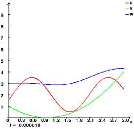
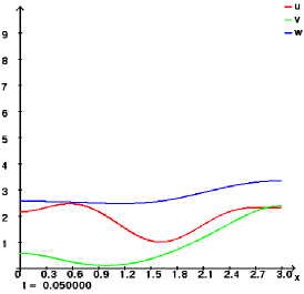
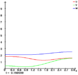
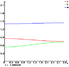
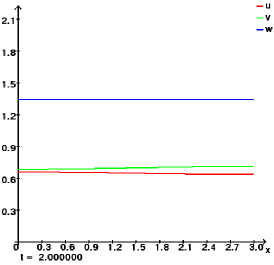
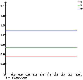
Figure 1: The expected solution behaviour

Because all parameters lie in the appropriate range, Theorem 1.1 verifies that the convergence observed is the correct long-term behaviour.

Second observation: Large $q_{i}$. Choosing $q_{1}=50$ and $q_{2}=0.1$, but otherwise the same parameters as in the first scenario, we witness the following “large-time” behaviour; pictures are taken at after 60000, 100000, 200000, 700000 time steps.

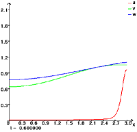
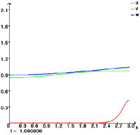
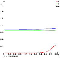
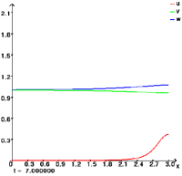
Figure 2: Large values of $q_{1}$.

The solutions still can be perceived to converge; however, the limiting profile is significantly different and not even spatially homogeneous, as can be seen in the last graph of Figure 2, where the solutions already have stabilized (which is indicated by the negligible changes between $t=2$ and $t=7$).

Whereas on the left part of the domain, the first species seems to have vanished entirely, it has survived on the right, lured there by the comparatively high concentrations of the chemoattractant which go back to the high initial deployment of the second species there.

Altogether, this contrasting appearance of the limit demonstrates that at least some smallness condition on $q_{1}$, $q_{2}$ is essential for the validity of the conclusion of Theorem 1.1.

Third observation: Behaviour on small time-scales. The following pictures are taken from the experiment performed for the second observation, that is for the same choice of parameters as in the preceding subsection. This time, we want to have a closer look at early solution behaviour and correspondingly in Fig. 3 depict the solution at time steps 500, 600, 676, 1400, 13000 and 30000.

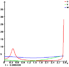
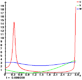
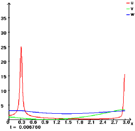
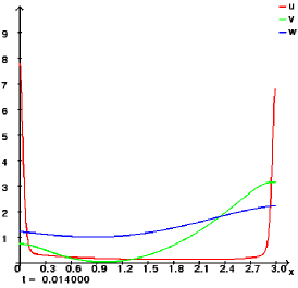
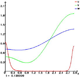
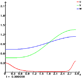
Figure 3: Solution at smaller times. (Note the changes of scale on the vertical axis.)

On these small time scale, that should be more representative for the actual dynamical evolution of species obeying model (1.2) that the large-time limiting behaviour of solutions, diverse phenomena occur. In Figure 3, the simultaneous emergence and movement of large aggregates of the chemotactically strongly active population can be observed as response to the emission of the joint signal by both species while they compete and the second population more slowly reacts to the same concentration gradients. It is worth noting that in this process astonishingly high concentrations can be reached; cf. Figure 4, where the spatial maxima of $u$ and $v$ are plottet versus time $t\in[0,0.02\ldots]$, and although the initial concentration $u_{0}$ was bounded from above by $3.5$, values of more than $150$ are attained. Therefore, it seems reasonable to expect results resembling those dealing with transient growth phenomena for single-species chemotaxis models [52, 22] also in the present two-species context.

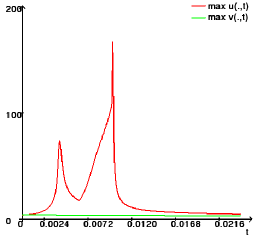
Figure 4: Evolution of the maximal population densities

Naturally, up to now analytical results (including those of the present article) have been confined to the solution behaviour in the limit $t\to\infty$, so that rigorous description and understanding of the intriguing performance of solutions over short periods of time remain as possibly worthwhile, albeit challenging, questions for future studies.

References

• [1]
• [2] M. Aida, T. Tsujikawa, M. Efendiev, A. Yagi, and M. Mimura. Lower estimate of the attractor dimension for a chemotaxis growth system. Journal of the London Mathematical Society, 74(2):453–474, 2006.
• [3] X. Bai and M. Winkler. Equilibration in a fully parabolic two-species chemotaxis system with competitive kinetics. 2016. preprint.
• [4] N. Bellomo, A. Bellouquid, Y. Tao, and M. Winkler. Toward a mathematical theory of Keller-Segel models of pattern formation in biological tissues. Math. Models Methods Appl. Sci., 25(9):1663–1763, 2015.
• [5] M. Bendahmane and M. Langlais. A reaction-diffusion system with cross-diffusion modeling the spread of an epidemic disease. J. Evol. Equ., 10(4):883–904, 2010.
• [6] P. Biler, E. E. Espejo, and I. Guerra. Blowup in higher dimensional two species chemotactic systems. Commun. Pure Appl. Anal., 12(1):89–98, 2013.
• [7] P. Biler and I. Guerra. Blowup and self-similar solutions for two-component drift-diffusion systems. Nonlinear Anal., 75(13):5186–5193, 2012.
• [8] R. S. Cantrell, C. Cosner, and Y. Lou. Advection-mediated coexistence of competing species. Proc. Roy. Soc. Edinburgh Sect. A, 137(3):497–518, 2007.
• [9] M. A. Chaplain and A. R. Anderson. Mathematical modelling of tissue invasion. Cancer modelling and simulation, pages 269–297, 2003.
• [10] F. Dickstein. Sharp conditions for blowup of solutions of a chemotactical model for two species in $\mathbb{R}^{2}$. J. Math. Anal. Appl., 397(2):441–453, 2013.
• [11] E. Espejo, K. Vilches, and C. Conca. Sharp condition for blow-up and global existence in a two species chemotactic Keller-Segel system in $\mathbb{R}^{2}$. European J. Appl. Math., 24(2):297–313, 2013.
• [12] E. E. Espejo, A. Stevens, and T. Suzuki. Simultaneous blowup and mass separation during collapse in an interacting system of chemotactic species. Differential Integral Equations, 25(3-4):251–288, 2012.
• [13] E. E. Espejo, A. Stevens, and J. J. L. Velázquez. A note on non-simultaneous blow-up for a drift-diffusion model. Differential Integral Equations, 23(5-6):451–462, 2010.
• [14] E. E. Espejo Arenas, A. Stevens, and J. J. L. Velázquez. Simultaneous finite time blow-up in a two-species model for chemotaxis. Analysis (Munich), 29(3):317–338, 2009.
• [15] B. S. Goh. Global stability in two species interactions. J. Math. Biol., 3(3-4):313–318, 1976.
• [16] T. Hillen and K. J. Painter. A user’s guide to PDE models for chemotaxis. J. Math. Biol., 58(1-2):183–217, 2009.
• [17] D. Horstmann. From 1970 until present: the Keller-Segel model in chemotaxis and its consequences. I. Jahresber. Deutsch. Math.-Verein., 105(3):103–165, 2003.
• [18] D. Horstmann. Generalizing the Keller-Segel model: Lyapunov functionals, steady state analysis, and blow-up results for multi-species chemotaxis models in the presence of attraction and repulsion between competitive interacting species. J. Nonlinear Sci., 21(2):231–270, 2011.
• [19] A. Kurganov and M. Lukáčová-Medviďová. Numerical study of two-species chemotaxis models. Discrete Contin. Dyn. Syst. Ser. B, 19(1):131–152, 2014.
• [20] M. Kurokiba. Existence and blowing up for a system of the drift-diffusion equation in $R^{2}$. Differential Integral Equations, 27(5-6):425–446, 2014.
• [21] K. Kuto, K. Osaki, T. Sakurai, and T. Tsujikawa. Spatial pattern formation in a chemotaxis-diffusion-growth model. Physica D: Nonlinear Phenomena, 241(19):1629 – 1639, 2012.
• [22] J. Lankeit. Chemotaxis can prevent thresholds on population density. Discrete and Continuous Dynamical Systems - Series B, 20(5):1499–1527, 2015.
• [23] J. Lankeit. Eventual smoothness and asymptotics in a three-dimensional chemotaxis system with logistic source. Journal of Differential Equations, 258(4):1158 – 1191, 2015.
• [24] D. Lauffenburger, R. Aris, and K. Keller. Effects of cell motility and chemotaxis on microbial population growth. Biophysical journal, 40(3):209, 1982.
• [25] D. A. Lauffenburger, M. Rivero, F. Kelly, R. Ford, and J. DiRienzo. Bacterial chemotaxis. Annals of the New York Academy of Sciences, 506(1):281–295, 1987.
• [26] Y. Li. Global bounded solutions and their asymptotic properties under small initial data condition in a two-dimensional chemotaxis system for two species. J. Math. Anal. Appl., 429(2):1291–1304, 2015.
• [27] Y. Li and Y. Li. Finite-time blow-up in higher dimensional fully-parabolic chemotaxis system for two species. Nonlinear Anal., 109:72–84, 2014.
• [28] J. Liu and C. Ou. How many consumer levels can survive in a chemotactic food chain? Front. Math. China, 4(3):495–521, 2009.
• [29] Y. Lou, Y. Tao, and M. Winkler. Approaching the ideal free distribution in two-species competition models with fitness-dependent dispersal. SIAM J. Math. Anal., 46(2):1228–1262, 2014.
• [30] S. Matsukuma and A. Durston. Chemotactic cell sorting in dictyostelium discoideum. Development, 50(1):243–251, 1979.
• [31] M. Mizukami and T. Yokota. Global existence and asymptotic stability of solutions to a two-species chemotaxis system with any chemical diffusion. 2016. preprint.
• [32] J. D. Murray. Mathematical Biology. II Spatial Models and Biomedical Applications $\{$Interdisciplinary Applied Mathematics V. 18$\}$. Springer-Verlag New York Incorporated, 2001.
• [33] E. Nakaguchi and M. Efendiev. On a new dimension estimate of the global attractor for chemotaxis-growth systems. Osaka Journal of Mathematics, 45(2):273–281, 06 2008.
• [34] E. Nakaguchi and K. Osaki. Global solutions and exponential attractors of a parabolic-parabolic system for chemotaxis with subquadratic degradation. Discrete Contin. Dyn. Syst. Ser. B, 18(10):2627–2646, 2013.
• [35] M. Negreanu and J. I. Tello. On a comparison method to reaction-diffusion systems and its applications to chemotaxis. Discrete Contin. Dyn. Syst. Ser. B, 18(10):2669–2688, 2013.
• [36] M. Negreanu and J. I. Tello. On a two species chemotaxis model with slow chemical diffusion. SIAM J. Math. Anal., 46(6):3761–3781, 2014.
• [37] M. Negreanu and J. I. Tello. Asymptotic stability of a two species chemotaxis system with non-diffusive chemoattractant. J. Differential Equations, 258(5):1592–1617, 2015.
• [38] K. J. Painter and T. Hillen. Spatio-temporal chaos in a chemotaxis model. Physica D: Nonlinear Phenomena, 240(4-5):363–375, 2011.
• [39] I. G. Pearce, M. A. Chaplain, P. G. Schofield, A. R. Anderson, and S. F. Hubbard. Chemotaxis-induced spatio-temporal heterogeneity in multi-species host-parasitoid systems. Journal of mathematical biology, 55(3):365–388, 2007.
• [40] C. Stinner, J. I. Tello, and M. Winkler. Competitive exclusion in a two-species chemotaxis model. J. Math. Biol., 68(7):1607–1626, 2014.
• [41] X. Tang and Y. Tao. Analysis of a chemotaxis model for multi-species host-parasitoid interactions. Appl. Math. Sci. (Ruse), 2(25-28):1239–1252, 2008.
• [42] Y. Tao and M. Winkler. Boundedness vs. blow-up in a two-species chemotaxis system with two chemicals. Discrete Contin. Dyn. Syst. Ser. B, 20(9):3165–3183, 2015.
• [43] J. I. Tello and M. Winkler. A chemotaxis system with logistic source. Comm. Partial Differential Equations, 32(4-6):849–877, 2007.
• [44] J. I. Tello and M. Winkler. Stabilization in a two-species chemotaxis system with a logistic source. Nonlinearity, 25(5):1413–1425, 2012.
• [45] B. Vasiev and C. J. Weijer. Modeling chemotactic cell sorting during dictyostelium discoideum mound formation. Biophysical journal, 76(2):595–605, 1999.
• [46] Q. Wang, J. Yang, and L. Zhang. Time periodic and stable patterns of a two–competing–species Keller–Segel chemotaxis model effect of cellular growth. ArXiv e-prints, May 2015.
• [47] Q. Wang, L. Zhang, J. Yang, and J. Hu. Global existence and steady states of a two competing species Keller-Segel chemotaxis model. Kinet. Relat. Models, 8(4):777–807, 2015.
• [48] W. Wang and Y. Li. Stabilization in an $n$-species chemotaxis system with a logistic source. J. Math. Anal. Appl., 432(1):274–288, 2015.
• [49] X. Wang and Y. Wu. Qualitative analysis on a chemotactic diffusion model for two species competing for a limited resource. Quart. Appl. Math., 60(3):505–531, 2002.
• [50] M. Winkler. Chemotaxis with logistic source: very weak global solutions and their boundedness properties. J. Math. Anal. Appl., 348(2):708–729, 2008.
• [51] M. Winkler. Boundedness in the higher-dimensional parabolic-parabolic chemotaxis system with logistic source. Comm. Partial Differential Equations, 35(8):1516–1537, 2010.
• [52] M. Winkler. How far can chemotactic cross-diffusion enforce exceeding carrying capacities? Journal of Nonlinear Science, pages 1–47, 2014.
• [53] G. Wolansky. Multi-components chemotactic system in the absence of conflicts. European J. Appl. Math., 13(6):641–661, 2002.
• [54] Q. Zhang and Y. Li. Global existence and asymptotic properties of the solution to a two-species chemotaxis system. J. Math. Anal. Appl., 418(1):47–63, 2014.
• [55] Q. Zhang and Y. Li. Global boundedness of solutions to a two-species chemotaxis system. Z. Angew. Math. Phys., 66(1):83–93, 2015.
• [56] Z. Zhang. Existence of global solution and nontrivial steady states for a system modeling chemotaxis. In Abstract and Applied Analysis, volume 2006. Hindawi Publishing Corporation, 2006.