Numerical test for hyperbolicity of chaotic dynamics in time-delay systems

Abstract

We develop a numerical test of hyperbolicity of chaotic dynamics in time-delay systems. The test is based on the angle criterion and includes computation of angle distributions between expanding, contracting and neutral manifolds of trajectories on the attractor. Three examples are tested. For two of them previously predicted hyperbolicity is confirmed. The third one provides an example of a time-delay system with nonhyperbolic chaos.

Hyperbolic chaotic attractors, like the Smale-Williams solenoid and some other mathematical examples, manifest deterministic chaos justified in rigorous mathematical sense Smale (1967); Anosov (1995); Katok and Hasselblatt (1995). In such attractors all orbits in state space are of saddle type, and their expanding and contracting manifolds do not have tangencies but can only intersect transversally. These attractors demonstrate strong stochastic properties and allow a detailed mathematical analysis. They are rough, i.e., structurally stable. This means robustness with respect to variation of functions and parameters in the dynamical equations, and insensitivity of chaos characteristics to noises, interferences etc. In the theory of oscillations, since the classic work of Andronov and his school Andronov and Pontryagin (1937); Andronov et al. (1966), rough or structurally stable systems are regarded as those subjected to priority research, and as the most important for practice. It seems natural that the same should be true for systems with structurally stable uniformly hyperbolic attractors. However, until very recently, no physical examples were known. The hyperbolic attractors were commonly regarded as purified abstract mathematical images of chaos rather than something intrinsic to real world systems. In this situation a good way was to turn to a purposeful construction of systems with hyperbolic dynamics using a toolbox of physics (oscillators, particles, fields, interactions, feedback circuits, etc.) instead of that of mathematics (geometric, algebraic, topological constructions). In this regard, certain progress has been achieved recently, and many realizable physically motivated systems with hyperbolic attractors have been offered Kuznetsov (2012, 2011).

Naturally, physical and technical devices we deal with are not well suited to allow mathematical proofs although confident confirmation of hyperbolicity is significant to exploit properly the relevant results of mathematical theory. So it is vital to employ numerical instruments for computational tests of hyperbolicity.

In this respect one has to mention first the so-called cone criterion based on a mathematical theorem adapted to computer verification that has been applied for some low-dimensional systems Kuznetsov and Sataev (2007); Kuznetsov et al. (2010); Wilczak (2010).

The second approach is based on the verification of transversality of stable and unstable manifolds for orbits belonging to the attractor, or more generally, to an invariant set of interest. It involves an inspection of statistical distributions of the angles between the manifolds. If hyperbolicity holds, all the observed angles have to be distant from zero. This method was suggested initially in Ref. Lai et al. (1993) and then developed and used with modifications in Hirata et al. (1999); Anishchenko et al. (2000); Kuznetsov (2005); Kuznetsov and Seleznev (2006); Ginelli et al. (2007); Wolfe and Samelson (2007); Kuptsov and Kuznetsov (2009); Kuptsov (2012); Kuptsov and Parlitz (2012); Kuznetsov (2015); Kuznetsov and Kruglov (2016). It may be regarded as an extended version of Lyapunov analyses, well-established and applied successively not only for low-dimensional systems but for spatiotemporal systems too.

An important class among nonlinear systems with complex dynamics is formed by systems containing time-delay feedback loops. Such examples are wide-spread in electronics, laser physics, acoustics and other fields Vyhlídal et al. (2013). An adequate mathematical description for these objects is based on differential equations with delays Bellman and Cooke (1963); Myshkis (1972); El’sgol’ts and Norkin (1973). These dynamical systems have to be treated as possessing infinite-dimensional state space since a continuum of data, i.e, a trajectory segment, determines each new infinitesimal time step. A number of time-delay systems with chaotic dynamics was explored Dorizzi et al. (1987); Chrostowski et al. (1983); Lepri et al. (1994); Mackey and Glass (1977); Farmer (1982); Grassberger and Procaccia (1984); Kuznetsov and Ponomarenko (2008); Kuznetsov and Pikovsky (2010, 2008); Baranov et al. (2010); Kuznetsov and Kuznetsov (2013). Several examples of them were suggested as realizable devices for generation of rough hyperbolic chaos Kuznetsov and Ponomarenko (2008); Kuznetsov and Pikovsky (2010, 2008); Baranov et al. (2010); Kuznetsov and Kuznetsov (2013). However, no computer verification of hyperbolicity was provided for these systems as no appropriate methods were elaborated for this special class of infinite-dimensional dynamics.

In the present paper we extend the angle criterion to make it applicable for time-delay systems with one constant retarding time.

To start with, let us recall the content of the angle criterion for finite-dimensional systems following Refs. Kuptsov (2012); Kuptsov and Parlitz (2012). For a system defined by a set of $m$ ordinary differential equations $\dot{X}=F(t,X)$ the corresponding variational equation for infinitesimal perturbations near the reference orbit $X(t)$ reads

$$\dot{x}=\mbox{\boldmath{$\mathrm{J}$}}(t)x,$$ (1)

where $X,x\in\mathbb{R}^{m}$ are the state vector and the perturbation vector, respectively, and $\mbox{\boldmath{$\mathrm{J}$}}(t)\in\mathbb{R}^{m\times m}$ is the Jacobi matrix. The notation $\mbox{\boldmath{$\mathrm{J}$}}(t)$ presumes the dependence of this matrix both on $t$ and $X(t)$. If the dependence of $F$ and, consequently, of $\mathrm{J}$ on $t$ is explicit, the system is nonautonomous. (In this case we always restrict ourselves to considering equations with periodic dependencies of coefficients on $t$.)

Assume that we deal with an invariant set (attractor) possessing $p$ positive, one zero, and $m-p-1$ negative Lyapunov exponents. To compute the angles between expanding, neutral, and contracting tangent subspaces we first need to run the standard algorithm for computing Lyapunov exponents Benettin et al. (1980); Shimada and Nagashima (1979). The main system is solved simultaneously with $p+1$ copies of the variational equation (1). Periodically perturbation vectors $x$ produced by the variational equations are orthogonalized and normalized. In matrix notation it corresponds to the so-called QR decomposition Golub and Van Loan (2012) of a $m\times(p+1)$ matrix whose columns are the perturbation vectors $x$. This procedure represents the matrix as a product of an orthogonal matrix $\mathrm{Q}$ and an upper triangle matrix $\mathrm{R}$. Often this is implemented via the Gram-Schmidt algorithm Golub and Van Loan (2012). The columns of $\mathrm{Q}$ are used in further computations as new perturbation vectors. After excluding transient iterations, they converge to the so-called backward Lyapunov vectors Kuptsov and Parlitz (2012) (they are called “backward” since arrive at $t$ after initialization in the far past; notice also that the convergence does not imply the time constancy of these vectors). Computing Lyapunov exponents, one accumulates logarithms of the diagonal elements of $\mathrm{R}$, but in the framework of the angle criterion one has to store the backward Lyapunov vectors instead. The time interval between successive QR decompositions can be chosen arbitrarily, but it must be not too large to avoid an overflow of computer digital registers. The backward Lyapunov vectors are stored for a discrete set of points where the angles will be computed later.

The next stage of the routine consists in the passage along the same reference orbit backward in time applying the similar Lyapunov algorithm but for $p+1$ vectors generated now by the adjoint variational equation

$$\dot{y}=-\mbox{\boldmath{$\mathrm{J}$}}^{*}(t)y.$$ (2)

Here $\mbox{\boldmath{$\mathrm{J}$}}^{*}(t)$ is the adjoint matrix for $\mbox{\boldmath{$\mathrm{J}$}}(t)$, such that the inner products involving arbitrary vectors $a$ and $b$ satisfy the identity $\langle\mbox{\boldmath{$\mathrm{J}$}}^{*}a,b\rangle\equiv\langle a,\mbox{\boldmath{$\mathrm{J}$}}b\rangle$. If the inner product is defined as $\langle a,b\rangle=b^{\text{T}}a$, then we have simply $\mbox{\boldmath{$\mathrm{J}$}}^{*}=\mbox{\boldmath{$\mathrm{J}$}}^{\text{T}}$, where “T” stands for transposition. The orthogonal matrices obtained from the QR procedure in the course of the computations with the adjoint equation (2) in backward time converge to the so-called forward Lyapunov vectors Kuptsov and Parlitz (2012).

Now we use the stored forward and backward Lyapunov vectors relating to the identical trajectory points. Information about the angles is encoded in a $(p+1)\times(p+1)$ matrix of their pairwise inner products. The smallest singular value $\sigma_{k}$ of its top left $k\times k$ submatrix is the tangency indicator: $\theta_{1}=\left(\pi/2-\arccos\sigma_{p}\right)$ is the angle between the expanding subspace and the sum of the neutral and contracting ones, and $\theta_{2}=\left(\pi/2-\arccos\sigma_{p+1}\right)$ is the angle between the expanding plus neutral subspace and the contracting one Kuptsov (2012).

One can easily check that for arbitrary solutions to Eqs. (1) and (2) the inner product remains constant in time, i.e., satisfies the identity

$$\frac{\mathrm{d}}{\mathrm{d}t}\left\langle x(t),y(t)\right\rangle\equiv 0.$$ (3)

In particular, in the case of nonzero inner product, if one of the solutions is characterized by a Lyapunov exponent so that $x(t)\sim\mathrm{e}^{\lambda t}$, then the other one has a Lyapunov exponent with the opposite sign, $y(t)\sim\mathrm{e}^{-\lambda t}$. Hence the Lyapunov spectra corresponding to equations (1) and (2) are identical up to the signs.

Given only one of Eqs. (1) and (2), one can use (3) to find the other one. This idea can be employed to recover a generic form of the adjoint variational equation for time delay systems.

Consider a time-delay system

$$\dot{X}=F(t,X,X_{\tau}),$$ (4)

where $X\equiv X(t)\in\mathbb{R}^{m}$, $X_{\tau}\equiv X(t-\tau)$, and $\tau$ is the delay time. The corresponding variational equation reads

$$\dot{x}=\mbox{\boldmath{$\mathrm{J}$}}_{x}(t)x(t)+\mbox{\boldmath{$\mathrm{J}$}}_{u}(t)x(t-\tau),$$ (5)

where $\mbox{\boldmath{$\mathrm{J}$}}_{x}(t)$ and $\mbox{\boldmath{$\mathrm{J}$}}_{u}(t)$ are the derivative matrices composed of partial derivatives of $F$ over components of $X$ and $X_{\tau}$, respectively.

As a preliminary step to guess a proper form for the adjoint variational equation we rewrite Eq. (5) as an equation for a system containing explicitly a delay line, where a signal propagation is characterized by the time $\tau$:

$$\dot{x}=\mbox{\boldmath{$\mathrm{J}$}}_{x}(t)x(t)+\mbox{\boldmath{$\mathrm{J}$}}_{u}(t)u(t,L),$$ (6)

$$u_{t}+u_{\xi}=\delta(\xi)x(t),$$ (7)

$$u(t,\xi<0)=0,\;u(t,\xi>0)=x(t-\xi).$$ (8)

Here $u\equiv u(t,\xi)$ is the delay line variable, $L=\tau$ is the length of the delay line, and the subscripts $t$ and $\xi$ stand for corresponding partial derivatives. The solution to Eq. (7) is a wave (8) propagating in the positive direction from a source at $\xi=0$. Substituting it into (6) yields the original equation (5).

In view of this recasting the variational equation, it is natural to define the inner product of two perturbation vectors $\bar{x}=(x,u)$ and $\bar{y}=(y,v)$ as

$$\langle\bar{x},\bar{y}\rangle=y^{\text{T}}(t)x(t)+\int\limits_{0}^{L}v^{\text{T}}(t,\xi)u(t,\xi)\,\mathrm{d}\xi.$$ (9)

The arbitrary solution $\bar{y}$ of desired adjoint variational equations and $\bar{x}$ satisfying Eqs. (6)-(8) have to fulfill a condition analogous to (3), i.e., $\mathrm{d}\left\langle\bar{x},\bar{y}\right\rangle/\mathrm{d}t\equiv 0$, with respect to the inner product (9). This requirement results in the following form of the adjoint variational equations:

$$\dot{y}=-\mbox{\boldmath{$\mathrm{J}$}}_{x}^{\text{T}}(t)y(t)-v(t,0),$$ (10)

$$v_{t}+v_{\xi}=\delta(\xi-L)\mbox{\boldmath{$\mathrm{J}$}}_{u}^{\text{T}}(t)y(t),$$ (11)

$$\begin{gathered}v(t,\xi>L)=0,\\ v(t,\xi<L)=\mbox{\boldmath{$\mathrm{J}$}}_{u}^{\text{T}}(t-\xi+L)y(t-\xi+L).\end{gathered}$$ (14)

(One can check directly that the identity $\mathrm{d}\left\langle\bar{x},\bar{y}\right\rangle/\mathrm{d}t\equiv 0$ is fulfilled taking into account the equality $(\mathrm{d}/\mathrm{d}t)\int_{0}^{L}f(t-\xi)\mathrm{d}\xi=f(t)-f(t-L)$.) Observe that, in contrast to Eq. (7) containing a source, we introduce a kind of sink in (11); in other words, we exploit here an advanced wave solution of equation (11) instead of the usual retarding wave solution.

Substituting Eq. (14) into (10), one can reformulate the adjoint variational problem as a differential equation with deviating argument:

$$\dot{y}=-\mbox{\boldmath{$\mathrm{J}$}}_{x}^{\text{T}}(t)y(t)-\mbox{\boldmath{$\mathrm{J}$}}_{u}^{\text{T}}(t+\tau)y(t+\tau).$$ (15)

The theory of differential equations with deviating arguments distinguishes three main cases: equations with a retarded argument (like Eqs. (4) and (5)), equations of neutral type (we do not deal with them here), and equations of leading or advanced type (like Eq. (15)) Bellman and Cooke (1963); Myshkis (1972); El’sgol’ts and Norkin (1973). The latter are regarded as poorly defined with respect to the existence of solutions to initial value problems. In the context of our study, however, we will solve such equations in backward time only, so that they behave in a good way like the equations of retarded type in forward time.

Notice that computing the inner products (9) of vectors obtained as trajectory segments of time duration $\tau$ produced by Eqs. (5) and (15), one needs to reverse the order of the adjoint trajectory variables: for Eq. (5) we set $[u(t,0),u(t,L)]=[x(t),x(t-\tau)]$, but for (15) $[v(t,0),v(t,L)]=[y(t+\tau),y(t)]$.

We will solve both Eq. (4) and the variational equation (5) numerically with Heun’s method that belongs to the class of second-order Runge-Kutta methods with constant time step Bellen and Zennaro (2013). The full state vector of the discrete time approximation of Eq. (5) includes $k+1$ elements $(x_{n-k},x_{n-k+1},\ldots,x_{n})$, where we assume $k=\tau/h$ to be an integer, and $h$ is a time step. Numerical integration of this linear equation implies successive multiplications of the state vector by a numerical Jacobi matrix $\mathrm{J}$ composed of $[m(k+1)]\times[m(k+1)]$ elements. Regardless of $k$, only a small number of the matrix elements are nontrivial; most of them are merely zeros and ones. In particular, for the Heun method this matrix has $3m^{2}$ nontrivial elements. In the course of the forward time stage of the angle computation algorithm one can store these matrix elements without the risk of exhausting a computer memory. Then, the backward time stage can be implemented without explicitly solving Eq. (15). One just computes adjoint matrices from the stored matrix elements and performs the iterations with them.

Computed in this way, the perturbation vectors converge as $h\to 0$ to solutions of Eqs. (5) and (15) if the adjoint numerical Jacobi matrix is defined as

$$\mbox{\boldmath{$\mathrm{\mbox{\boldmath{$\mathrm{J}$}}}$}}^{*}=\mbox{\boldmath{$\mathrm{H}$}}^{-2}\mbox{\boldmath{$\mathrm{\mbox{\boldmath{$\mathrm{J}$}}}$}}^{\text{T}}\mbox{\boldmath{$\mathrm{H}$}}^{2},$$ (16)

where $\mbox{\boldmath{$\mathrm{H}$}}=\mathop{\mathrm{diag}}(1,\sqrt{h},\ldots,\sqrt{h})$ and $\mbox{\boldmath{$\mathrm{H}$}}^{2}$ is a metric tensor generated by a discrete version of the inner product (9);

$$\langle\bar{x},\bar{y}\rangle=y^{\text{T}}_{n}x_{n}+h\sum\limits_{i=1}^{k}v^{\text{T}}_{i}u_{i}=y^{\text{T}}\mbox{\boldmath{$\mathrm{H}$}}^{2}x.$$ (17)

Here $u_{i}=x_{n-i}$, and if $v_{i}$ corresponds to an adjoint vector, the elements of the backward in time solution $y_{i}$ have to be taken in the reverse order: $v_{i}=y_{n+k+1-i}$.

Orthonormalization routines employed in the angle computations have to be re-implemented according to the nonstandard form of the inner product (17). When exploiting linear algebra libraries, a simpler alternative is to change the basis for the perturbation vectors setting $a^{\prime}=\mbox{\boldmath{$\mathrm{H}$}}a$ with respective transformation of the Jacobi matrix

$$\mbox{\boldmath{$\mathrm{J}$}}^{\prime}=\mbox{\boldmath{$\mathrm{H}$}}\,\mbox{\boldmath{$\mathrm{J}$}}\,\mbox{\boldmath{$\mathrm{H}$}}^{-1}.$$ (18)

One can see that $a^{\text{T}}\,\mbox{\boldmath{$\mathrm{H}$}}^{2}b=(a^{\prime})^{\text{T}}b^{\prime}$, and $b=\mbox{\boldmath{$\mathrm{J}$}}a$ is equivalent to $b^{\prime}=\mbox{\boldmath{$\mathrm{J}$}}^{\prime}a^{\prime}$. In other words, the transformed Jacobi matrix $\mbox{\boldmath{$\mathrm{J}$}}^{\prime}$ and the corresponding vectors are written in orthonormal basis whose metric tensor is the identity. Altogether, computing the Jacobi matrices along a forward time trajectory we first transform them according to Eq. (18) and then perform the angle computation algorithm implementing standard orthonormalization routines without the need to redefine the inner product.

Now we are ready to apply the angle criterion to particular time-delay systems.

The first is a nonautonomous system based on the van der Pol oscillator of natural frequency $\omega_{0}$ supplied with a specially designed time-delay feedback Kuznetsov and Ponomarenko (2008):

$$\ddot{X}-[A\cos(2\pi t/T)-X^{2}]\dot{X}+\omega_{0}^{2}X=\epsilon X_{\tau}\dot{X}_{\tau}\cos\omega_{0}t.$$ (19)

The parameter controlling the oscillator excitation is modulated with period $T$ and amplitude $A$. Accordingly, the oscillator alternately manifests activation and damping. If the retarding time $\tau$ is properly tuned, say $\tau=\frac{3}{4}T$, the emergence of self-oscillations at each next stage of activity is stimulated by a signal emitted at the previous activity stage. Since the delayed signal is squared and mixed with auxiliary oscillations of frequency $\omega_{0}$, the stimulating force has again frequency $\omega_{0}$, but the doubled phase in comparison with the original oscillations. As a result, we get a sequence of oscillation trains with phases at successive excitation stages obeying the doubly-expanding circle map that is a chaotic Bernoulli-type map

$$\phi_{n+1}=2\phi_{n}+\mathrm{const}\mod 2\pi.$$ (20)

According to argumentation in Ref. Kuznetsov and Ponomarenko (2008), this means that the attractor for a Poincaré map, which corresponds to states obtained stroboscopically at $t_{n}=nT$, is of Smale-Williams type, and the respective chaotic dynamics is hyperbolic. (In fact, the system (19) has an additional attracting fixed point $X=0$, but its basin of attraction is very narrow. Arbitrarily chosen initial conditions of relatively large amplitude provide an approach of orbits to the Smale-Williams attractor.)

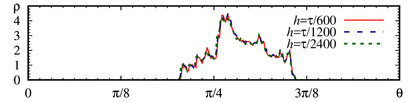
Figure 1: (color online) Distributions of $\theta_{1}$ for system (19) at different time steps $h$, see the legend. $T=6$, $\tau=\frac{3}{4}T$, $A=4.7$, $\epsilon=0.3$, $\omega_{0}=2\pi$. The first four Lyapunov exponents are $0.114$,$-0.139$,$-0.714$, $-0.801$.

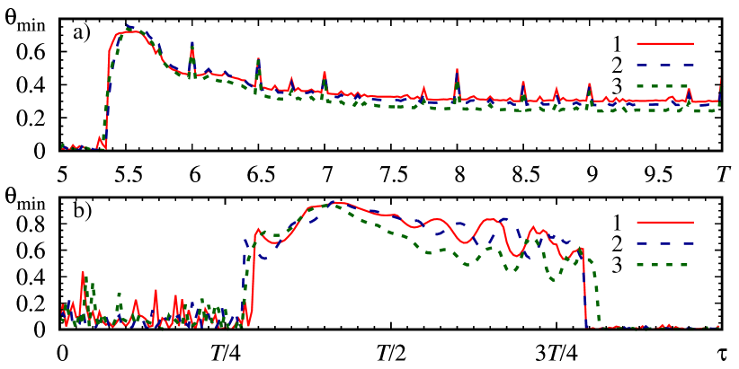
Figure 2: (color online) The minimum cutoff angle $\theta_{\text{min}}$ against (a) $T$ and (b) $\tau$. (a) $\tau=3T/4$. Curve 1: $A=4.7$, $\epsilon=0.3$; 2: $A=5$, $\epsilon=0.25$; 3: $A=5.5$, $\epsilon=0.2$. (b) Curve 1: $A=4.7$, $\epsilon=0.3$, $T=6$; 2: $A=5$, $\epsilon=0.2$, $T=6.5$; 3: $A=5.2$, $\epsilon=0.15$, $T=7.5$. For both panels $\omega_{0}=2\pi$.

The system (19) has a single positive Lyapunov exponent and the others are negative. (Zero Lyapunov exponent is absent because of the nonautonomous nature of the system.) Thus, we need to implement the angle computation routine with $p=1$.

Figure 1 shows histograms of the angle distributions computed for numerical solutions of the equations with different time steps $h$. The angles are obtained for the corresponding stroboscopic map at $t=t_{0}+nT$, where $t_{0}$ is large enough to exclude transients, and $n=0,1,2,\ldots$. Regardless of $h$ (being sufficiently small) the distributions have a well reproducible form that supports the correctness of our definitions in the continual limit. The form of the histograms certainly confirms the hyperbolicity of chaotic dynamics in the system. Indeed, the distribution is well separated from zero angles.

Figure 2 shows the dependencies of the minimum cut-off angle $\theta_{\text{min}}$ against the system parameters to verify robustness of the hyperbolic chaos. In its panels (a) and (b) $T$ and $\tau$ are varied, respectively, for three arbitrarily chosen sets of parameters. Observe that the angle distributions remain well separated from the origin in a wide parameter domain. (The spikes on the curves in panel (a), e.g., at $T=6,6.5,7$ etc., correspond to situations when the angle distributions are maximally distant from zero, although it is not easy to explain the origin of the phenomenon clearly.) In the left part of the plot (a) relating to the case $\tau=\frac{3}{4}T$ one can see a narrow domain where the minimal angles are close to zero, and the dynamics becomes nonhyperbolic. In panel (b) an extensive domain of hyperbolicity in the middle part shows that the fine tuning of $\tau$ at given $T$ is actually not necessary because the hyperbolicity persists in a relatively wide range.

The second system we consider is an autonomous model with an attractor of Smale-Williams type suggested in Ref. Kuznetsov and Pikovsky (2010), see also Kuznetsov (2012); Arzhanukhina and Kuznetsov (2014):

$$\dot{X} =-\omega_{0}Y+\tfrac{1}{2}\mu(1-X^{2}_{\tau}-Y^{2}_{\tau})X+\epsilon X_{\tau}Y_{\tau},$$ (21)

$$\dot{Y} =\phantom{-}\omega_{0}X+\tfrac{1}{2}\mu(1-X^{2}_{\tau}-Y^{2}_{\tau})Y.$$

Here $\mu$ is an excitation parameter and $\omega_{0}$ can be treated as a natural frequency. When $\epsilon=0$, this system generates trains of oscillations of frequency $\omega_{0}$ periodically alternating with damping stages of very low amplitude. Due to the term providing a delayed feedback controlled by the small parameter $\epsilon$, each new train of oscillations arises from a seed signal produced by the system at the previous excitation stage. Because of the quadratic nonlinearity of the respective term, each time the phase is doubled in comparison with the previous one. As a result, the phases at successive excitation stages evolve according to the Bernoulli-type map (20), and, as argued in Ref. Kuznetsov and Pikovsky (2010), this means that the Poincaré map constructed for the system (21) has an attractor of Smale-Williams type. Following Kuznetsov and Pikovsky (2010), we will consider the Poincaré map on the surface $X^{2}+Y^{2}=1$ taking into account the passages of phase trajectories in the direction of increasing amplitude and computing the angles between subspaces there.

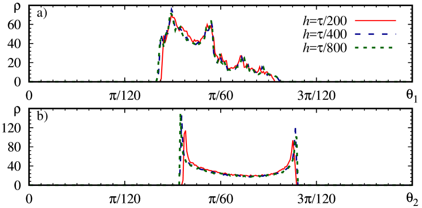
Figure 3: (color online) Distributions of the first (a) and second (b) angles for the Poincaré map of the autonomous system (21) computed at different time steps, see the legend. $\mu=1.6$, $\omega_{0}=2\pi$, $\epsilon=0.05$, $\tau=2$. The first four Lyapunov exponents are $0.060$, $0$, $-1.938$, $-2.463$.

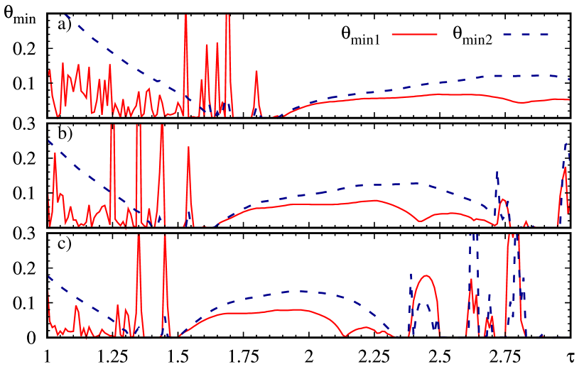
Figure 4: (color online) First and second minimum cutoff angles vs. delay time $\tau$ at various parameters: (a) $\mu=1.6$, $\epsilon=0.05$; (b) $\mu=1.8$, $\epsilon=0.07$; (c) $\mu=2$, $\epsilon=0.03$. For all panels $\omega_{0}=2\pi$.

Autonomous system (21) has a single positive Lyapunov exponent, a zero one, and the other exponents are negative. The zero Lyapunov exponent and the corresponding neutral subspace vanish for the Poincaré map, so that one can consider only the angles between the expanding and contracting subspaces as above. However, implementing this approach, one needs to project the computed perturbation vectors onto the section surface and then evaluate the angles between these projections. A simpler way is to consider perturbation vectors as they appear in computations in full phase space and to check both the angles $\theta_{1}$ (the expanding subspace vs. the sum of neutral and contracting subspaces) and $\theta_{2}$ (the expanding plus neutral subspace vs. the contracting subspace). Chaos is hyperbolic when both of these angles never vanish.

Figure 3 shows histograms of the distributions of these angles obtained for certain parameters of the system (see the caption) at different values of the integration step $h$. We see a good convergence as $h\to 0$ both for $\theta_{1}$ and for $\theta_{2}$ (panels (a) and (b), respectively). Both distributions are well separated from the zero angle having clearly expressed cutoffs that confirms hyperbolicity of the attractor. The robustness of this regime is illustrated in Fig. 4(a-c), which represents the dependence of the minimum cutoff angles $\theta_{\text{min}1}$ and $\theta_{\text{min}2}$ versus the parameter of time delay $\tau$ for three sets of other parameters. On all three plots well-defined ranges occur corresponding to domains of existence of the hyperbolic attractor where both angles are well detached from zero.

The last example we present is aimed to outline the difference between the hyperbolic and nonhyperbolic chaos. It is the well-known Mackey-Glass system Mackey and Glass (1977); Farmer (1982); Grassberger and Procaccia (1984)

$$\dot{X}=aX_{\tau}/\left(1+X_{\tau}^{10}\right)-bX,$$ (22)

where $a=0.2$ and $b=0.1$. When $\tau>17$, chaotic oscillations occur in the system Farmer (1982); Grassberger and Procaccia (1984).

To perform an adequate comparison with the previous cases, we have to introduce for this system an appropriate Poincaré section providing well-expressed separation of the successive crossings by phase trajectories. A good and satisfactory expedient is based on complementing the model (22) with an auxiliary equation $\tau\dot{Y}=X-X_{\tau}-Y$ and locating the section surface at $Y=0$. The variable $Y$ roughly follows $X$ but smoothes out its high-frequency fluctuations.

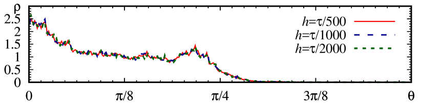
Figure 5: (color online) Distribution of $\theta_{1}$ for system (22) at different time steps, see the legend. $\tau=23$. The first four Lyapunov exponents are $0.0096$, $0$, $-0.0114$, $-0.0350$.

Figure 5 shows histograms for the angle $\theta_{1}$ between the expanding subspace and the sum of neutral and contracting subspaces for the attractor observed at $\tau=23$. The attractor has one positive, one zero, and other negative Lyapunov exponents. Observe the clearly expressed violation of hyperbolicity: the distributions demonstrate a significant probability of angles close to zero, which implies occurrence of tangencies for the subspaces. It is a sufficient condition to judge about the absence of hyperbolicity, so that there is no need to analyze a distribution for $\theta_{2}$.

To conclude, we have developed the method of hyperbolicity verification based on the angle criterion for time-delay systems, which may be regarded as an extension of numerical Lyapunov analysis. Three particular examples have been tested. For two of them the previously believed hyperbolicity has been confirmed and for the third one the nonhyperbolic nature of the generated chaos has been established. We have restricted ourselves here to considering systems with one delay time. Extension for two or more delays requires further elaboration of the algorithm.

As regards the theoretical foundation and general formulation of the method, the work was supported by RSF grant No 15-12-20035 (SPK). The work of elaborating computer routines and numerical computations for particular examples was supported by RFBR grant No 16-02-00135 (PVK).

References

- Smale (1967) S. Smale, “Differentiable dynamical systems,” Bull. Amer. Math. Soc. (NS) 73, 747–817 (1967).
- Anosov (1995) D. V. Anosov, ed., Dynamical Systems 9: Dynamical Systems with Hyperbolic Behaviour, Encyclopaedia Math. Sci., Vol. 9 (Berlin: Springer, 1995).
- Katok and Hasselblatt (1995) A. Katok and B. Hasselblatt, Introduction to the Modern Theory of Dynamical Systems, 1st ed., Encyclopedia of mathematics and its applications, Vol. 54 (Cambridge University Press, 1995) p. 802.
- Andronov and Pontryagin (1937) A. A. Andronov and L. S. Pontryagin, “Structurally stable systems,” in Dokl. Akad. Nauk SSSR, Vol. 14 (1937) pp. 247–250.
- Andronov et al. (1966) A. A. Andronov, S. E. Khaikin, and A. A. Vitt, Theory of Oscillators (Pergamon Press, 1966).
- Kuznetsov (2012) S. P. Kuznetsov, Hyperbolic Chaos: A Physicist’s View (Higher Education Press: Bijing and Springer-Verlag: Berlin, Heidelberg, 2012) p. 336.
- Kuznetsov (2011) S. P. Kuznetsov, “Dynamical chaos and uniformly hyperbolic attractors: From mathematics to physics,” Phys. Uspekhi. 54, 119–144 (2011).
- Kuznetsov and Sataev (2007) S. P. Kuznetsov and I. R. Sataev, “Hyperbolic attractor in a system of coupled non-autonomous van der pol oscillators: Numerical test for expanding and contracting cones,” Phys. Lett. A 365, 97–104 (2007).
- Kuznetsov et al. (2010) A. S. Kuznetsov, S. P. Kuznetsov, and I. R. Sataev, “Parametric generator of hyperbolic chaos based on two coupled oscillators with nonlinear dissipation,” Tech. Phys. 55, 1707–1715 (2010).
- Wilczak (2010) D. Wilczak, “Uniformly hyperbolic attractor of the Smale–Williams type for a Poincaré map in the Kuznetsov system,” SIAM J. Applied Dynamical Systems 9, 1263–1283 (2010).
- Lai et al. (1993) Y.-C. Lai, C. Grebogi, J. A. Yorke, and I. Kan, “How often are chaotic saddles nonhyperbolic?” Nonlinearity 6, 779–798 (1993).
- Hirata et al. (1999) Y. Hirata, K. Nozaki, and T. Konishi, “The intersection angles between N-dimensional stable and unstable manifolds in 2N-dimensional symplectic mappings,” Prog. Theor. Phys. 102, 701–706 (1999).
- Anishchenko et al. (2000) V. S. Anishchenko, A. S. Kopeikin, J. Kurths, T. E. Vadivasova, and G. I. Strelkova, “Studying hyperbolicity in chaotic systems,” Phys. Lett. A 270, 301–307 (2000).
- Kuznetsov (2005) S. P. Kuznetsov, “Example of a physical system with a hyperbolic attractor of the smale-williams type,” Phys. Rev. Lett. 95, 144101 (2005).
- Kuznetsov and Seleznev (2006) S. P. Kuznetsov and E. P. Seleznev, “A strange attractor of the smale–williams type in the chaotic dynamics of a physical system,” JETP 102, 355–364 (2006).
- Ginelli et al. (2007) F. Ginelli, P. Poggi, A. Turchi, H. Chaté, R. Livi, and A. Politi, “Characterizing dynamics with covariant lyapunov vectors,” Phys. Rev. Lett. 99, 130601 (2007).
- Wolfe and Samelson (2007) C. L. Wolfe and R. M. Samelson, “An efficient method for recovering Lyapunov vectors from singular vectors,” Tellus A 59, 355–366 (2007).
- Kuptsov and Kuznetsov (2009) P. V. Kuptsov and S. P. Kuznetsov, “Violation of hyperbolicity in a diffusive medium with local hyperbolic attractor,” Phys. Rev. E 80, 016205 (2009).
- Kuptsov (2012) P. V. Kuptsov, “Fast numerical test of hyperbolic chaos,” Phys. Rev. E 85, 015203 (2012).
- Kuptsov and Parlitz (2012) P. V. Kuptsov and U. Parlitz, “Theory and computation of covariant Lyapunov vectors,” J. Nonlinear. Sci. 22, 727–762 (2012).
- Kuznetsov (2015) S. P. Kuznetsov, “Hyperbolic chaos in self-oscillating systems based on mechanical triple linkage: Testing absence of tangencies of stable and unstable manifolds for phase trajectories,” Regular and Chaotic Dynamics 20, 649–666 (2015).
- Kuznetsov and Kruglov (2016) S. P. Kuznetsov and V. P. Kruglov, “Verification of hyperbolicity for attractors of some mechanical systems with chaotic dynamics,” Regular and Chaotic Dynamics 21, 160–174 (2016).
- Vyhlídal et al. (2013) T. Vyhlídal, J. F. Lafay, and R. Sipahi, eds., Delay Systems: From Theory to Numerics and Applications, Vol. 1 (Springer Science & Business Media, 2013).
- Bellman and Cooke (1963) R. Bellman and C.L. Cooke, Differential-difference equations (Acad. Press, 1963).
- Myshkis (1972) A.D. Myshkis, Linear differential equations with retarded argument (Moscow, Nauka, 1972) p. 352, in Russian.
- El’sgol’ts and Norkin (1973) L.E. El’sgol’ts and S.B. Norkin, Introduction to the theory and application of differential equations with deviating arguments (Acad. Press, 1973) p. 356.
- Dorizzi et al. (1987) B. Dorizzi, B. Grammaticos, M. LeBerre, Y. Pomeau, E. Ressayre, and A. Tallet, “Statistics and dimension of chaos in differential delay systems,” Phys. Rev. A 35, 328–339 (1987).
- Chrostowski et al. (1983) J. Chrostowski, R. Vallee, and C. Delisle, “Self-pulsing and chaos in acoustooptic bistability,” Can. J. Phys. 61, 1143–1148 (1983).
- Lepri et al. (1994) S. Lepri, G. Giacomelli, A. Politi, and F. T. Arecchi, “High-dimensional chaos in delayed dynamical systems,” Phys. D 70, 235–249 (1994).
- Mackey and Glass (1977) MC Mackey and L Glass, “Oscillation and chaos in physiological control systems,” Science 197, 287–289 (1977).
- Farmer (1982) J. D. Farmer, “Chaotic attractors of an infinite-dimensional dynamical system,” Phys. D 4, 366–393 (1982).
- Grassberger and Procaccia (1984) P. Grassberger and I. Procaccia, “Dimensions and entropies of strange attractors from a fluctuating dynamics approach,” Phys. D 13, 34–54 (1984).
- Kuznetsov and Ponomarenko (2008) S. P. Kuznetsov and V. I. Ponomarenko, “Realization of a strange attractor of the Smale-Williams type in a radiotechnical delay-feedback oscillator,” Tech. Phys. Lett. 34, 771–773 (2008).
- Kuznetsov and Pikovsky (2010) S. P. Kuznetsov and A. Pikovsky, “Attractor of Smale-Williams type in an autonomous time-delay system,” Preprint nlin. arXiv: 1011.5972 (2010).
- Kuznetsov and Pikovsky (2008) S. P. Kuznetsov and A. Pikovsky, “Hyperbolic chaos in the phase dynamics of a q-switched oscillator with delayed nonlinear feedbacks,” Europhys. Lett. 84 (2008).
- Baranov et al. (2010) S. V. Baranov, S. P. Kuznetsov, and V. I. Ponomarenko, “Chaos in the phase dynamics of q-switched van der pol oscillator with additional delayed-feedback loop,” Izvestiya VUZ. Applied Nonlinear Dynamics (Saratov) 18, 11–23 (2010), in Russian.
- Kuznetsov and Kuznetsov (2013) A. S. Kuznetsov and S. P. Kuznetsov, “Parametric generation of robust chaos with time-delayed feedback and modulated pump source,” Commun. Nonlinear Sci. Numer. Simul. 18, 728–734 (2013).
- Benettin et al. (1980) Giancarlo Benettin, Luigi Galgani, Antonio Giorgilli, and Jean-Marie Strelcyn, “Lyapunov characteristic exponents for smooth dynamical systems and for hamiltonian systems: a method for computing all of them. Part 1: Theory,” Meccanica 15, 9–20 (1980).
- Shimada and Nagashima (1979) Ippei Shimada and Tomomasa Nagashima, “A numerical approach to ergodic problem of dissipative dynamical systems,” Prog. Theor. Phys. 61, 1605–1616 (1979).
- Golub and Van Loan (2012) Gene H Golub and Charles F Van Loan, Matrix computations, Vol. 3 (JHU Press, 2012).
- Bellen and Zennaro (2013) Alfredo Bellen and Marino Zennaro, Numerical methods for delay differential equations (Oxford university press, 2013) p. 410.
- Arzhanukhina and Kuznetsov (2014) D. S. Arzhanukhina and S. P. Kuznetsov, “Robust chaos in autonomous time-delay system,” Izvestiya VUZ. Applied Nonlinear Dynamics (Saratov) 22, 36–49 (2014).