GPU-FV: Realtime Fisher Vector and Its Applications in Video Monitoring

Abstract

Fisher vector has been widely used in many multimedia retrieval and visual recognition applications with good performance. However, the computation complexity prevents its usage in real-time video monitoring. In this work, we proposed and implemented GPU-FV, a fast Fisher vector extraction method with the help of modern GPUs. The challenge of implementing Fisher vector on GPUs lies in the data dependency in feature extraction and expensive memory access in Fisher vector computing. To handle these challenges, we carefully designed GPU-FV in a way that utilizes the computing power of GPU as much as possible, and applied optimizations such as loop tiling to boost the performance. GPU-FV is about 12 times faster than the CPU version, and 50% faster than a non-optimized GPU implementation. For standard video input (320*240), GPU-FV can process each frame within 34ms on a model GPU. Our experiments show that GPU-FV obtains a similar recognition accuracy as traditional FV on VOC 2007 and Caltech 256 image sets. We also applied GPU-FV for realtime video monitoring tasks and found that GPU-FV outperforms a number of previous works. Especially, when the number of training examples are small, GPU-FV outperforms the recent popular deep CNN features borrowed from ImageNet.

1 Introduction

Many recent research show that Fisher vector [30] is a very useful representation of images, which obtains state-of-the-art results in a number of applications, including image retrieval [22, 10], art classification [19], relevance feedback of videos [13], event recounting in videos [29], texture recognition [6], face verification [26], object detection [5, 33], and fine grained image recognition[12, 23]. Although the recent deep convolutional neural network [16] outperforms Fisher vector in large scale visual recognition challenges such as ImageNet LSVRC [9], the training process of deep CNN usually requires a lot of training examples. In scenarios where the training set is in small or middle scale, Fisher vector is still a very attractive choice, especially when the problem lies in a different domain from the existing large scale dataset.

However, Fisher vectors pose an even heavier computational demand, which limits its usage in real world applications. It takes about 2-5 seconds for a typical implementation of Fisher vector to classify a normal sized image. Such a slowness prevents Fisher vectors from many real applications. To bridge the gap, this paper proposes GPU-FV, an efficient implementation of Fisher vector with the help of GPUs .

It is not trivial to write efficient GPU code for Fisher vector, because of the data dependency in dense SIFT, and the complicated memory access patterns in GMM estimation. To overcome this challenge, we not only design efficient kernels to explore the parallel nature in SIFT extraction, but also formulate GMM estimation in a way that can utilize the limited bandwidth and memory in modern GPUs. We propose several techniques to optimize the feature extraction speed: (1) Loop tiling, (2) early termination, and (3) vectorization, and (4) using 8 scales for dense SIFT exatraction. We demonstrate that our optimization technique can speed up a naive Fisher vector implementation on GPUs by more than 20 times.

Some techniques in optimizing the GPU computation bring approximation of the computation. To evaluate the effects of these approximations, we compare our GPU implementation with the original Fisher vector on two standard datasets: PASCAL VOC 2007 and Caltech 256. The results show that our approximate obtain a similar accuracy but with a much higher speed. We believe such evaluation provides strong evidence that our GPU based Fisher vector can be used for many applications.

Our GPU-FV system can process a 320 * 240 image in 34ms. Such an efficiency makes it possible to employ Fisher vector to realtime applications. To demonstrate it, this paper shows an example of applying an abnormal event detector in realtime surveillance videos, and an example of detecting baby’s laugh in a video. In surveillance and video recognition, existing solutions are very slow and it is difficult to apply them to online processing scenarios. However, this paper demonstrates that our new GPU based Fisher vector can model complicated subjects and obtain an accuracy comparable with the the state-of-the-art.

2 Related Works

GPUs have been evolving fast, and have been applied in high performance computing successfully. However, it remains unclear what are the bottlenecks in accurate visual categorization with the Fisher vector model on GPU.

SURF is an optimized robust feature extraction system [1]. Cornelis and Van Gool [8] implemented SURF on the GPU (Graphics Processing Unit) and obtained an order of magnitude speedup compared to a CPU implementation. Extracting SIFT descriptors on GPU has been studied by other researchers [28, 35]. Recent efforts were also made on accelerating Dense SIFT computation [21]. SVM model training, have been independently studied on the GPU before [3]. To address the bottlenecks in accurate visual categorization systems, Sande et.al [32] did a detailed analysis, and proposed two GPU-accelerated algorithms, GPU vector quantization and GPU kernel value precomputation, which results in a substantial acceleration of the complete visual categorization pipeline. However, their method does not involve Fisher vector encoding.

Efforts have been made to reduce the storage and computation overhead of Fisher vector [22], by compressing the Fisher vector, with some loss of precision. The widely used Vlfeat package  [34] provides a wonderful implementation of the Fisher vector, along with other popular computer vision algorithms. However, there was no GPU-based implementation in this package. A few years back, some researchers implemented Fisher vector on GPU [2], but it is on a modified algorithm with hierarchical GMM model, and the accuracy is lower than the state-of-the-art.

The problem of abnormal event recognition in videos has attracted many attentions [37] [15] [17]. However, the approaches listed above did not use Fisher Vector due to its slowness. Chen et al. [4] used MoSIFT and Fisher Vector for event detection, and obtained good performance on TRECVID data. However, their work did not consider how to speed up local feature extraction or Fisher vector encoding. As a result, their method relies on significant subsampling of one from 30/60/120 frames and the time of encoding such a frame is about 0.4 second (with feature extraction it will be longer). We believe our work in this paper can be easily employed by the framework [4] and provide similar speed up. Oneata et al. also used Fisher Vector in action localization and event recognition [20], at a speed 2.4 times slower than real-time. In this paper, we demonstrate that with GPU based Fisher Vector, we can handle some abnormal event recognition very well at a realtime speed.

In recent years, deep neural network have enjoyed a remarkable success as efficient and effective in a number of visual recognition tasks [27, 31]. Especially, Razavian et al. [24] showed that by simply borrowing the CNN-based AlexNet model [16] trained for ImageNet, a SVM model using CNN features can obtain the state-of-the-art in many applications. The deep CNN features could be sped up significantly by GPUs. We believe Fisher vector can be sped up with the same hardware, and in this paper we show that GPU-FV can outperform deep CNN features in some applications with limited amount of training samples.

3 GPU-FV

In this section, we will first introduce the Fisher vector algorithm and then explain our GPU-based implementation in detail.

3.1 Overview of Fisher Vector

There are two main computation components when generating Fisher vector for a picture. The first component is extracting the dense SIFT descriptors. An image is scaled to different sizes. Descriptors are extracted for all the scales. For each scale, the gradients of the pixels fall into 8 orientation bins. Then, the convolution kernels are applied. After that, each value in the 8 orientation bins is multiplied with the weights computed for each of the 16 spatial bin (4 on X and 4 on Y dimension). Therefore, a 128 dimension descriptor(8*4*4) is generated for each pixel. Then, by lowering the dimension to $m$ ($m<$128) with PCA and adding the normalized X and Y axis, a descriptor with dimension $M$=$m$+2 is generated for a pixel. The descriptors are extracted with a stride of $S$ on X and Y dimension, which means we get a descriptor in every $S^{2}$ pixels.

The second component is using the descriptors to generate the Fisher vectors with the GMM components trained beforehand. With the $means$, $covariances$, and $priors$ values of GMM, the dense SIFT descriptors are used to generate a Fisher vector for an image. The algorithm is described in Algorithm 1 [30]. Generating the Fisher vector includes two phases. In the first phase, we get the posteriors for each descriptor regarding the GMM components. In the second phse, the Fisher vector for the image is generated, represented as the concatenation of vectors $V$ and $U$ in Algorithm 1. $V$ and $U$ are of size $M$*$N$, where $M$ is the dimension of a descriptor, and $N$ is the number of GMM components.

Algorithm 1 Fisher Vector Encoding Algorithm

0:  Dense SIFT descriptors $data$

0:  GMM model: $means$, $covariances$, $priors$

0:  Fisher Vector: $V$,$U$

1:  Compute $\sqrt{{\sigma}^{-1}}$

2:  for $i=0$ to $num\_descriptors$ do

3:     for $j=0$ to $num\_components$ do

4:        $t$=distance(${data[i]},{means_{j}},{covariances_{j}}$);

5:        Compute $posteriors_{i,j}$ with $temp$;

6:        $maxPost$ = max{$maxPost$, $posteriors_{i,j}$};

7:     end for

8:     for $j=0$ to $num\_components$ do

9:        $posterior_{i,j}$ = $e^{posterior_{i,j}-maxPost}$;

10:        $sum$ += $posterior_{i,j}$;

11:     end for

12:     for $j=0$ to $num\_components$ do

13:        $posterior_{i,j}$ = $posterior_{i,j}/sum$;

14:     end for

15:  end for

16:  for $i=0$ to $num\_descriptors$ do

17:     for $j=0$ to $num\_components$ do

18:        if $posterior_{i,j}>$threshold then

19:           for $k=0$ to $DIMENSION$ do

20:              $U_{j,k}$+=$(data[i][k]-means_{j,k})*\sqrt{{\sigma}^{-1}}*posteriors_{i,j}$;

21:              $V_{j,k}$+=$(((data[i][k]-means_{j,k})*\sqrt{{\sigma}^{-1}})^{2}-1)*posteriors_{i,j}$;

22:           end for

23:        end if

24:     end for

25:  end for

3.2 The Parallelization Scheme on GPU

In this section, we describe the implementation details of the GPU-FV system.

Terminology First, we introduce some terminology to be used when describing GPU programs. A GPU kernel is a function launched by the CPU and run on the GPU. A kernel is run by a $thread\ grid$, which consists of a bunch of $thread\ blocks$. Each $block$ is comprised with a certain number of threads. Threads in the same block run on the same multiprocessor in a GPU, and share a piece of scratchpad memory, called $shared\ memory$, which could be read and written by the program, and is much faster than the GPU device memory. Threads are scheduled as $warps$, which is a bunch of threads that run in a SIMD fashion. With conditional branches such as “if…else…”, if the condition varies among threads in the same warp, the whole warp must go through both branches.

Dense SIFT on GPU There are two types of dense SIFT extracting methods: flat window and Gaussian window. In flat window dense SIFT, the triangular convolution kernels are used, and the convolution routine need to be called only twice (once on each dimension) for the 8 gradient bin, therefore reducing the amount of computation. To leverage this optimization, we implemented our GPU code based on the flat window dense SIFT algorithm. However, the original CPU implementation cannot be changed to GPU code directly because of its sequential nature. The triangular convolution involves 4 steps: (1) integrate backward the column, (2) compute the filter forward, (3) integrate forward the column, and (4) compute the filter backward. The first and third steps are accumulations, while the second and the fourth steps are subtraction operations. Each step is a $scan$ operation in nature, as shown in Step 1 in Figure 1. Because the computation of $b[i]$ depends on the result of $[i-1]$ computed in the last iteration, the computation of $b[i]$ and $b[i-1]$ cannot be done in parallel. $Scan$ operation need aggressive optimization when implemented on GPU to gain performance benefits [36], and $scan$ with subtraction is even harder to be implemented on GPU.

With careful examination, we found that there is useless computation in this process, because some data are added (in step 1 or 3), then subtracted (in step 2 or 4). Therefore, we revised the algorithm into a 2-step procedure, by combining the first two steps, and the last two steps. In each of the two steps, GPU threads sum up only the needed f data for each output point, where f is the filter size. Figure 1 shows this combination. The red squares are inputs to the first step. The green squares are the results after the adding operation in Step 1. The yellow squares are the results after two steps, which is the $scan$ operation with subtraction. The window size is 2. By combining Step 1 and Step 2, we got a simplified computation pattern, as shown in the “Combined Step”. Now the subtraction operation is not required any more. This algorithm could run efficiently on GPU. We spread the threads in each thread block on the columns of an image, and let each thread block process one column of the image. Thus, each thread does the convolution for a pixel by doing two rounds of adding operations, with $f$ adding operations in a round. Threads in the same block use the shared memory to buffer the data in the same column of the image, to accelerate data access.

We also optimized the GPU computation by removing computation for unused pixels. As mentioned in Section 3.1, the descriptors are extracted with a step of 4 on X and Y dimension, which means we need only 1 descriptor in every 16 pixels. In the original code, all the pixels are processed with both of the two convolution operations. In the GPU code, we reduced computation time by computing only the required data in the second convolution.

Generating the dense SIFT descriptors need preprocessing of images, such as image resizing, computation of gradients, normalization, etc. These steps are easy to be implemented as GPU kernels. With the preprocessing done on GPU, we were able to avoid extra data copy from host memory to GPU memory.

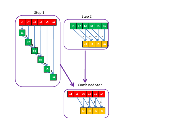
Figure 1: Combining two steps in Dense SIFT

Algorithm 2 GPU code for Phase 1

0:  Dense SIFT descriptors $data$

0:  GMM model: $means$, $covariances$, $priors$

1:  //Each block processes one descriptor at a time

2:  for $i=0$ to $num\_descriptors$  do

3:     Load all dimensions of $data[i]$ to shared memory;

4:     Synchronize();

5:     for $j=0$ to $num\_components$ do

6:        //Thread $k$ processes $data[i][k]$

7:        $t$=distance($data[i][k]$, $means_{j,k}$, $covariances_{j,k}$ );

8:        Sum up $t$ from all the threads in the block in a tree structure;

9:        Synchronize();

10:        if ThreadID==0 then

11:           Compute $posteriors_{i,j}$ with $t$;

12:           $maxPost$ = max{$maxPost$, $posteriors_{i,j}$};

13:        end if

14:        Synchronize();

15:     end for

16:     //Each thread processes one component at a time

17:     for $j=0$ to $num\_components$  do

18:        $posterior_{i,j}$ = $e^{posterior_{i,j}-maxPost}$;

19:        $sum$ += $posterior_{i,j}$;

20:     end for

21:     Synchronize();

22:     Sum up $sum$ with all the threads in the block in a tree structure;

23:     Synchronize();

24:     //Each thread processes one component at a time

25:     for $j=0$ to $num\_components$  do

26:        $posterior_{i,j}$ = $posterior_{i,j}/sum$;

27:     end for

28:  end for

Algorithm 3 GPU code for Phase 2

1:  //Each block processes one descriptor at a time

2:  for $i=0$ to $num\_descriptors$  do

3:     Load all dimensions of $data[i]$ and $posterior_{i}$ to shared memory;

4:     for $j=0$ to $num\_components$ do

5:        //Thread $k$ processes $data[i][k]$

6:        if $posterior_{i,j}>threshold$ then

7:           $U_{j,k}$+=$(data[i][k]-means_{j,k})*\sqrt{{\sigma}^{-1}}*posterior_{i,j}$;

8:           $V_{j,k}$+=$(((data[i][k]-means_{j,k})*\sqrt{{\sigma}^{-1}})^{2}-1)*posterior_{i,j}$;

9:        end if

10:     end for

11:  end for

12:  //Start a new kernel for accumulation of $U$ and $V$

13:  //Each block processes $U$ and $V$ for one GMM component

14:  for $i=1$ to $num\_blocks$  do

15:     //Thread $k$ processes $U_{j,k}$ and $V_{j,k}$

16:     $U_{j,k}$+=the $i$th copy of $U_{j,k}$

17:     $V_{j,k}$+=the $i$th copy of $V_{j,k}$

18:  end for

Generating Fisher Vector on GPU

The GPU implementation of the two phases is shown in Algorithm 2 and 3 respectively. In Phase 1, the posterior values are calculated for each descriptor. Phase 2 generates Fisher vector based on the posteriors. Therefore, both phases involve an outer loop on the number of descriptors. So it is natural to parallelize the outer loop (the loop on the number of descriptors) at block level on GPU. It means thread block $i$ processes $data[i*CHUNK]$ to $data[(i+1)*CHUNK]$ by looping through the $CHUNK$ descriptors. An important factor affecting performance is the choice of $CHUNK$. We will explain how we choose this value later in this section. Now let us look at the implementation of Phase 1 first. Algorithm 2 describes the implementation of the main kernel on GPU, and before this function starts, $\sqrt{{\sigma}^{-1}}$ has been computed with a simple GPU kernel. In this phase, the most time consuming computation is calculating the distances between the descriptor and each GMM component. We parallelized this computation at thread level. For each GMM component, every thread processes one dimension of the descriptor, and obtain the distance value in that dimension. The results of all the threads are summed up by a tree structured reduction operation, to obtain the final distance value of this descriptor.(Intuitively, we could let each thread process all the dimensions for each GMM component, therefore avoiding the need for reduction on the computation of distances. However, we found that the parallelization on the inner loops is more beneficial, because it enables coalesced access to global memory, and avoids bank conflicts when accessing shared memory.)

At the end of the reduction process, Thread 0 would have the distance value for the descriptor. Then Thread 0 computes the posterior value for the descriptor, and updates $maxPost$.

After that, the posteriors are updated with the exponential operation, as in Line 17 in Algorithm 2. Then, to get the summation of the posteriors for all the components, a new round of reduction is conducted. Finally, we are able to get the normalized posterior values by dividing the posteriors with the sum.

In the second phase, we compute the Fisher vector (U and V) with the posteriors. Similar to the first phase, each thread block processes $CHUNK$ descriptors assigned to it in a loop. Every thread computes one dimension in U[j] and V[j] at a time. As shown in Line 7 and 8 in Algorithm 3, the calculated values are used to update U and V. A challenge in updating U and V values on GPU is that all the blocks are updating the same elements in U and V. To solve this problem, we keep one copy of U and V for each block, and every blocks only updates its own copy. When this kernel finishes, each block has computed the values of U and V regarding the posteriors that it process. Then, we launch a new kernel to sum up the $U$ and $V$ copies updated by each block, to obtain the final Fisher vector.

The descriptor and the posterior values are buffered in shared memory, since they can be reused when processing each component, as Line 3 in Algorithm 3.

Now let us revisit the problem of choosing the values of $CHUNK$. We used different $CHUNK$ values for the two phases. This is because Phase 2 needs to accumulate the $U$ and $V$ values calculated from each descriptor. Having a large $CHUNK$ implies fewer thread blocks, because each block processes more data. Therefore, we will have less copies of $U$ and $V$, reducing the overhead of summing up values from different blocks. On the other hand, using small $CHUNK$ number for Phase 1 will enable better load balance and higher level of parallelism, so we chose a smaller $CHUNK$ size for Phase 1. Different $CHUNK$ values imply different thread block numbers, therefore we launch a separate kernel for each phase. By testing with different values, we chose $CHUNK$=4 in Phase 1, and $CHUNK$=192 in Phase 2 in our experiments.

3.3 Optimizing GPU Implementation

Loop tiling As a common optimization in CPU code, loop tiling turned out to be an effective optimization for GPU code also. Normally, loop tiling improves performance by reducing the number of conditional checking. In our case, this technique provides more benefit by avoiding a number of synchronizations among threads in a block. As shown in Algorithm 2, we need synchronizations before and after thread 0 computes the posteriors. Besides, there is a synchronization operation after reduction on every level. Suppose there are 10 synchronizations in the loop body. If we tile the loop by 4, the total number of synchronizations in 4 iterations is still 10, therefore the number of synchronizations is reduced by 75%.

In the first phase, we tiled the outer loop by 4, which means each block processes 4 descriptors at a time. The inner loop, which is on the number of components, is tiled by 2. The loops in the second phase are also tiled. The outer loop (on the number of descriptors) is tiled by 2, and the inner loop (on the number of components) is tiled by 4.

Early termination of an iteration In the second phase, we were able to apply early termination of an iteration by checking conditions in a clustered way. In the original algorithm, if the posterior of a certain point is less than a threshold, the value does not need to be added, as Line 18 in Algorithm 1. In the tiled GPU code, each block processes 8 posteriors in one iteration, so we load the $means$ value to shared memory for computation before processing the descriptors, since the $means$ values could be reused. However, we noticed that the posterior values are very sparse, therefore, if all the 8 values in an iteration are below the threshold, we can simply skip the iteration, as shown in Algorithm 5. In this case, we avoided the loading of $means$ for this iteration, and we combined the 8 branches into one branch, which is beneficial to GPU code because of its SIMD nature.

Vectorization Vectorization is an importation optimization for modern GPU. With loop unrolling, each thread is processing multiple data elements, therefore we pack the operation on multiple data elements into a vector operation. For example, when computing the distance between a data point and a component, the loop is unrolled with a factor of 4. Therefore we use vector operations on vectors with 4 float point data. By applying vectorization to the computation of posteriors on GPU, we were able to further improve the performance.

Figure 2 shows the effectiveness of the optimization. The bars with “no optimization” means the code without optimization. The bars labeled “Loop tiling” are running time with loop tiling. Bars with “Early termination” represents timing with both loop tiling and early termination, and those labeled with “Vectorization” are timing with all the three optimization methods. Since there are many synchronizations in Phase 1, it gains a good deal of performance improvement from loop tiling. Early termination applies only to Phase 2. Because there are many small posterior values, the early termination is very effective in reducing the time of Phase 2. Vectorization gave a further improvement for Phase 1, which has a good amount of dense computation.

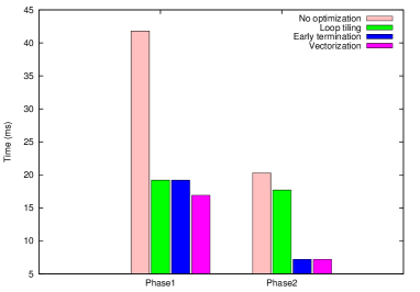
Figure 2: Performance improvement with the optimization

Algorithm 4 Basic loop structure of Phase 2 on GPU

1:  for $i=0$ to $num\_descriptors$, $step$ = 2 do

2:     for $j=0$ to $num\_components$, $step$ = 4 do

3:        if $posterior_{i,j}>threshold$  then

4:           Compute $U$ and $V$ values

5:        end if

6:        if $posterior_{i,j+1}>threshold$  then

7:           Compute $U$ and $V$ values

8:        end if$\cdots$

9:     end for

10:  end for

Algorithm 5 Optimized loop structure of Phase 2 on GPU

1:  for $i=0$ to $num\_descriptors$, $step$ = 2 do

2:     for $j=0$ to $num\_components$, $step$ = 4 do

3:        bool $b1$ = $posterior_{i,j}<1e-6$;

4:        bool $b2$=$posterior_{i,j+1}<1e-6$;

5:        $\cdots$

6:        bool $TotalB$=$b1\&b2\&b3...b8$;

7:        if $TotalB>0$ then

8:           continue;

9:        end if

10:        if $posterior_{i,j}>threshold$ then

11:           Compute $U$ and $V$ values

12:        end if

13:        if $posterior_{i,j+1}>threshold$  then

14:           Compute $U$ and $V$ values

15:        end if$\cdots$

16:     end for

17:  end for

4 Experiments

We evaluated our GPU-FV system in two scenarios. The first scenario is image classification with Fisher vector. The second part is event/expression detection in video, using Fisher vector generated for each frame. The testing platform is a dual CPU computer, which has two Intel Xeon E5-2630 v3 CPUs at clock rate of 2.40GHz, with 8 cores on each. It has an NVIDIA Tesla K40 card, with CUDA 7.0 installed. We used the same encoding scheme as VLFeat, with 256 GMM components, and 82 dimension dense SIFT descriptors at a stride of 4 on each dimension of the original image. The 9 scales of an image are selected from 2 to 1/8, with a decreasing factor of $\sqrt{2}$.

4.1 Comparing GPU-FV with Fisher vectors on CPUs

We tested our GPU code on the PASCAL VOC2007 and Caltech256 image sets. We compare GPU-FV with the MATLAB CPU code in VLFeat. The same encoding and classification algorithms are used in all the versions. The average encoding time for each image is plotted in Figure 3, and the accuracy values in mAP are listed in Table 2. For the CPU code, since VLFeat provided OPENMP implementation, we tested it on 1 thread and 16 threads, shown as the first two bars in each cluster of Figure 3. To show the effectiveness of the optimization to the GPU code, we included tests on GPU with and without the optimizations mentioned in Section 3.3, plotted as the two bars labeled “GPU 9 scales no optimization” and “GPU 9 scales”. By “9 scales”, we mean that dense SIFT is extracted from 9 scales of an image, which is the original setting in VLFeat. For the GPU code, we also tested the version with 8 scales in dense SIFT by removing the largest scale (resized to 2 times of the image), shown as the last bar in each cluster of the figure. Using 8 scales and with all the optimization strategies, the average encoding time for each image is 77.58ms for the VOC2007 set, and 53.99ms for the CalTech256 set. We did this test to show that this approximation (removing one scale) could improve performance dramatically, while maintaining about the same accuracy.

The tests on VOC2007 used 5011 images for training the svm classifier, and used another 4952 images as testing set. The average encoding time for each picture is shown in the left cluster of bars in Figure 3. Our optimized GPU code got a speedup of 12.68 over the 1 thread CPU code, and 4.53 over the 16 thread CPU code. The optimization of GPU code improves performance by 53.5% over the unoptimized version. The tests on 8 scales further reduced the running time by 48%, but the accuracy is not affected by removing one scale. The accuracy of each class is shown in Table 1.

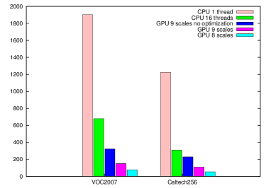
Figure 3: Average encoding time for each image

Table 1: The accuracy of each class in VOC2007

class	CPU	GPU
	9scales	8scales
	(%)	(%)
aeroplane	82.90	81.75
bicycle	65.44	65.52
bird	57.40	52.93
boat	72.94	72.60
bottle	27.12	28.03
bus	65.32	67.01
car	81.51	81.45
cat	57.56	55.97
chair	50.92	45.89
cow	43.60	43.45
diningtable	58.00	55.51
dog	41.84	41.05
horse	81.84	81.07
motorbike	66.64	68.67
person	84.97	84.51
pottedplant	30.19	27.88
sheep	48.30	46.33
sofa	56.70	53.56
train	82.07	81.63
tvmonitor	52.98	51.16

Table 2: The accuracy of different versions

Data set	CPU	GPU	GPU
		9scales	8scales
VOC2007 (mAP)	59.93%	59.03%	59.3%
Caltech256 (accuracy)	42.08%	42.88%	39.48%

The test on Caltech256 uses 7680 images for training, and 6400 images for testing, with more diversity in image size and shape. The performance is shown in the 5 bars on the right in Figure 3. The GPU code got a speedup of 21.8 over the 1 thread version, and 5.53 over the 16 thread version. The optimization reduced average running time on 9 scales GPU code by 52.5%. The accuracy on 8 scales is still acceptable, while the time is reduced by 50%.

4.2 Applications for Real Time Video Monitoring

In our tests with Caltech256 set, we found that the encoding time on GPU is a few dozens of milli-seconds for small pictures. Therefore, we try to apply GPU-FV to real-time video processing scenarios. By encoding each frame in a video, various classification and detection jobs could be conducted. We show two experiments on video processing in this paper. In detecting abnormal events, we used the GMM components trained in the Caltech256 experiment to generate Fisher vectors for the frames. For baby laughing detection, we used GMM components trained from random samples in pubfig, which is a data set with pictures of human faces.

In the first experiment, we tried to detect abnormal events from the UMN crowd activity video. The video consists of 3 scenes. In each scene, people are walking casually or standing. At a certain time, all the people are running away in various directions. The three scenes are in different places, with different light conditions. Each frame has a label to denote whether it is in the abnormal event. The frames with people running are labeled as “abnormal events”. Figure 4 shows a frame without any abnormal event on the left, and a scene with abnormal event on the right. The resolution of the video is 320*240 pixels.

In each scene, we used the first 700 frames to train a classification model with liblinear [11]. Then we use the model to predict abnormal events in the scene.

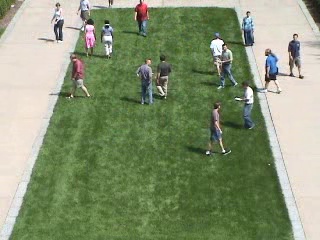
Figure 4: Example frames for UMN abnormal event dataset.

In the experiments, we used 8 scales for dense SIFT descriptors, and the total encoding time for each frame is 34ms on average. It means that we can process about 29 frames in a second, implying that we can apply the classification to real-time usage. We compare the performance of our GPU-FV with some well-known event detection methods in Table 3, with the last column listing the time for generating feature for each frame (or for each segment for C3D). C3D generates feature for every segment of 16 frames, so we evaluated its AUC with prediction for both segment level and frame level. It can be seen that our GPU-FV is much faster than the traditional event detection methods.

Table 3: The performance on UMN dataset (three scenes together).

Method	AUC	Encoding Time
Our GPU-FV	0.984	0.034s
Deep CNN feature [14]	0.930	0.020s
sparse reconstruction cost [7]	0.978	0.8s
local statistical aggregates [25]	0.985	1.1s
social force [18]	0.960	5s
C3D [31]	0.945(segment)	0.053s
C3D [31]	0.946(frame)	0.053s

Deep CNN features with Caffe is the only one that outperforms GPU-FV in encoding time, but at a lower AUC value. Figure 5 compares the prediction values using GPU-FV and deep CNN features [24] on the three scenes. We presented the prediction values from liblinear with the red star lines. The blue lines depict the ground truth, in which a value “1” represents an abnormal event. In the 3 graphs on the left, which are results using GPU-FV, it can be seen that the bursts with high value in the red start lines are consistent with the periods in which the blue lines are with value “1”. And it is clear that GPU-FV outperforms deep CNN features by providing clearer distinction between normal scenes and abnormal scenes. The average AUC (area under ROC curve) for GPU-FV is 0.984, while the average AUC for deep features is 0.930. The reason why deep feature does not work well for this problem is because the number of training examples in the classification of frames in a video is too small. In addition, the scenario of abnormal event detection is very different from ImageNet objects, where the deep CNN features are trained from.

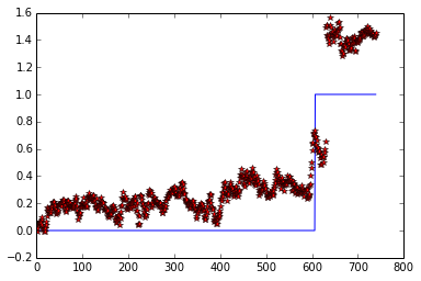
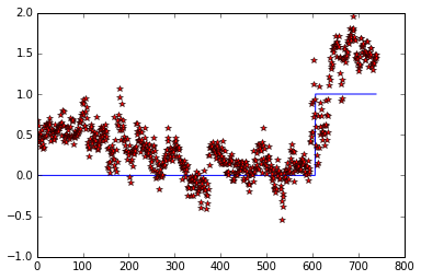
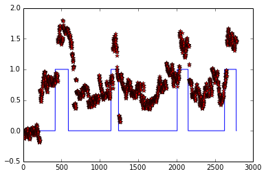
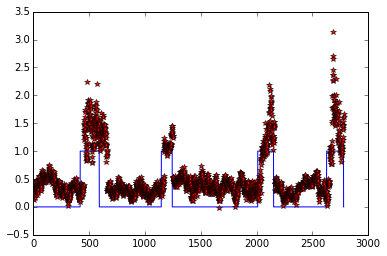
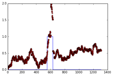
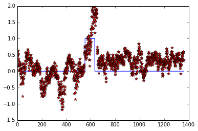
Figure 5: Comparing the prediction values using GPU-FV (left) and deep CNN feature (trained from ImageNet using AlexNet).

Another experiment we did is detecting baby’s laugh from a video. The video is also of resolution 320*240. We labeled the frames when a baby is laughing as 1, and the other frames as 0. The left picture in Figure 6 shows a frame when the baby is laughing, the one on the right is a frame when the baby is not laughing. Similar to the first experiment, we used the first 700 frames as training set, and used the following frames as testing set. We also tested this video using CNN from Caffe [14] and C3D [31], with performance comparison listed in Table 4. It shows that though encoding on Caffe is faster, our method obtained a much higher accuracy than CNN features (0.935 compared to 0.655). And because we extracted features for each frame, we got a much higher AUC than C3D when evaluated at frame level.

Figure 6: Example frames of baby expression video.

Table 4: The performance on detecting baby’s laugh.

Method	AUC	Encoding time
Our GPU-FV	0.935	0.034 s
Deep CNN feature [14]	0.655	0.020 s
C3D [31]	0.914(segment)	0.083 s
C3D [31]	0.593(frame)	0.083 s

5 Conclusion

In this paper, we introduced an optimized implementation of Fisher vector on GPU (GPU-FV), and showed its application to image classification and events detection in videos. Our method demonstrated a promising approach to using Fisher vector for real-time video processing. In future, we plan to expand the algorithm to more applications in video processing, to provide support for real-time situations.

6 Acknowledgments

This work is supported by the National High-tech R&D Pro- gram of China (No. 2012AA 010902), and the National Natural Science Foundation of China (No. 61303059).

References

- [1] H. Bay, A. Ess, T. Tuytelaars, and L. V. Gool. SURF: Speeded up robust features. In Computer Vision and Image Understanding (CVIU), 2008.
- [2] E. Bodzsar, B. Daroczy, I. Petras, and A. A. Benczur. GMM based fisher vector calculation on GPGPU. 2011.
- [3] B. Catanzaro, N. Sundaram, and K. Keutzer. Fast support vector machine training and classification on graphics processors. In ICML, 2008.
- [4] Q. Chen, Y. Cai, L. Brown, A. Datta, Q. Fan, R. Feris, S. Yan, A. Hauptmann, and S. Pankanti. Spatio-temporal fisher vector coding for surveillance event detection. In Proceedings of the 21st ACM International Conference on Multimedia, MM ’13, pages 589–592, New York, NY, USA, 2013. ACM.
- [5] Q. Chen, Z. Song, R. Feris, A. Datta, L. Cao, Z. Huang, and S. Yan. Efficient maximum appearance search for large-scale object detection. In IEEE Conference on Computer Vision and Pattern Recognition, pages 3190–3197, 2013.
- [6] M. Cimpoi, S. Maji, I. Kokkinos, S. Mohamed, and A. Vedaldi. Describing textures in the wild. In IEEE Conference on Computer Vision and Pattern Recognition, 2014.
- [7] Y. Cong, J. Yuan, and J. Liu. Sparse reconstruction cost for abnormal event detection. In IEEE Conference on Computer Vision and Pattern Recognition, pages 3449–3456, 2011.
- [8] N. Cornelis and L. V. Gool. Fast scale invariant feature detection and matching on programmable graphics hardware. In CVPR workshop, 2008.
- [9] J. Deng, W. Dong, and et al. ImageNet: A Large-Scale Hierarchical Image Database. In CVPR, 2009.
- [10] M. Douze, A. Ramisa, and C. Schmid. Combining attributes and Fisher vectors for efficient image retrieval. In CVPR 2011 - IEEE Conference on Computer Vision & Pattern Recognition, pages 745–752, Colorado Springs, United States, June 2011. IEEE.
- [11] R.-E. Fan, K.-W. Chang, C.-J. Hsieh, X.-R. Wang, and C.-J. Lin. LIBLINEAR: A library for large linear classification. In Journal of Machine Learning Research, 2008.
- [12] E. Gavves, B. Fernando, C. G. Snoek, A. W. Smeulders, and T. Tuytelaars. Fine-grained categorization by alignments. In Computer Vision (ICCV), 2013 IEEE International Conference on, pages 1713–1720. IEEE, 2013.
- [13] J. U. N. S. Ionuţ Mironică, Bogdan Ionescua. Fisher kernel based relevance feedback for multimodal video retrieval. In Computer Vision and Image Understanding, Feb 2016.
- [14] Y. Jia, E. Shelhamer, J. Donahue, S. Karayev, J. Long, R. Girshick, S. Guadarrama, and T. Darrell. Caffe: Convolutional architecture for fast feature embedding. arXiv preprint arXiv:1408.5093, 2014.
- [15] L. Kratz and K. Nishino. Anomaly detection in extremely crowded scenes using spatio-temporal motion pattern models. In CVPR, pages 1446–1453, 2009.
- [16] A. Krizhevsky, I. Sutskever, and G. E. Hinton. ImageNet classification with deep convolutional neural networks. In NIPS, pages 1106–1114, 2012.
- [17] C. Lu, J. Shi, and J. Jia. Abnormal event detection at 150 fps in matlab. In ICCV, pages 2720–2727, 2013.
- [18] R. Mehran, A. Oyama, and M. Shah. Abnormal crowd behavior detection using social force model. In IEEE Conference on Computer Vision and Pattern Recognition, pages 935–942, 2009.
- [19] T. E. J. Mensink and J. C. van Gemert. The rijksmuseum challenge: Museum-centered visual recognition. In ACM International Conference on Multimedia Retrieval, 2014.
- [20] D. Oneata, J. Verbeek, and C. Schmid. Action and Event Recognition with Fisher Vectors on a Compact Feature Set. In ICCV 2013 - IEEE International Conference on Computer Vision, pages 1817–1824, Sydney, Australia, Dec. 2013. IEEE.
- [21] D. Patlolla, S. Voisin, H. Sridharan, and A. Cheriyadat. GPU accelerated textons and dense sift features for human settlement detection from high-resolution satellite imagery. In GeoComp, 2015.
- [22] F. Perronnin, Y. Liu, J. Sánchez, and H. Poirier. Large-scale image retrieval with compressed fisher vectors. In Computer Vision and Pattern Recognition (CVPR), 2010 IEEE Conference on, pages 3384–3391. IEEE, 2010.
- [23] H. J. F. P. Philippe-Henri Gosselina, Naila Murrayc. Revisiting the fisher vector for fine-grained classification. In Pattern Recognition Letters, Nov 2014.
- [24] A. S. Razavian, H. Azizpour, J. Sullivan, and S. Carlsson. CNN features off-the-shelf: an astounding baseline for recognition. CVPRW DeepVision workshop, 2014.
- [25] V. Saligrama and Z. Chen. Video anomaly detection based on local statistical aggregates. In IEEE Conference on Computer Vision and Pattern Recognition, pages 2112–2119, 2012.
- [26] K. Simonyan, O. M. Parkhi, A. Vedaldi, and A. Zisserman. Fisher vector faces in the wild. In Proc. BMVC, volume 1, page 7, 2013.
- [27] K. Simonyan and A. Zisserman. Two-stream convolutional networks for action recognition in videos. In NIPS, 2014.
- [28] S. Sinha, J.-M. Frahm, M. Pollefeys, and Y. Genc. Feature tracking and matching in video using programmable graphics hardware. Machine Vision and Applications, 22(1):207–217, 2011.
- [29] C. Sun, B. Burns, R. Nevatia, C. Snoek, B. Bolles, G. Myers, W. Wang, and E. Yeh. ISOMER: Informative segment observations for multimedia event recounting. In Proceedings of International Conference on Multimedia Retrieval, ICMR ’14, pages 241:241–241:248, New York, NY, USA, 2014. ACM.
- [30] J. Sánchez, F. Perronnin, T. Mensink, and J. Verbeek. Image Classification with the Fisher Vector: Theory and Practice. In International Journal of Computer Vision, 2013.
- [31] D. Tran, L. Bourdev, R. Fergus, L. Torresani, and M. Paluri. Learning spatiotemporal features with 3D convolutional networks. In ICCV, 2015.
- [32] K. E. A. van de Sande, T. Gevers, and C. G. M. Snoek. Empowering visual categorization with the GPU. IEEE Transactions on Multimedia, 13(1):60–70, 2011.
- [33] K. E. A. van de Sande, C. G. M. Snoek, and A. W. M. Smeulders. Fisher and VLAD with FLAIR. In CVPR, 2014.
- [34] A. Vedaldi and B. Fulkerson. VLFeat: An open and portable library of computer vision algorithms. http://www.vlfeat.org, 2008.
- [35] W. Wang, Y. Zhang, G. Long, S. Yan, and H. Jia. CLSIFT: An optimization study of the scale invariance feature transform on GPUs. In HPCC 2013.
- [36] S. Yan, G. Long, and Y. Zhang. StreamScan: fast scan algorithms for GPUs without global barrier synchronization. In ACM SIGPLAN Symposium on Principles and Practice of Parallel Programming, PPoPP ’13, Shenzhen, China, February 23-27, 2013, pages 229–238, 2013.
- [37] B. Zhao, L. Fei-Fei, and E. P. Xing. Online detection of unusual events in videos via dynamic sparse coding. In CVPR, pages 3313–3320, 2011.