Recency-Bounded Verification of Dynamic Database-Driven Systems
(Extended Version)

Abstract

We propose a formalism to model database-driven systems, called database manipulating systems (DMS). The actions of a DMS modify the current instance of a relational database by adding new elements into the database, deleting tuples from the relations and adding tuples to the relations. The elements which are modified by an action are chosen by (full) first-order queries. DMS is a highly expressive model and can be thought of as a succinct representation of an infinite state relational transition system, in line with similar models proposed in the literature. We propose monadic second order logic (MSO-FO) to reason about sequences of database instances appearing along a run. Unsurprisingly, the linear-time model checking problem of DMS against MSO-FO is undecidable. Towards decidability, we propose under-approximate model checking of DMS, where the under-approximation parameter is the “bound on recency”. In a $k$-recency-bounded run, only the most recent $k$ elements in the current active domain may be modified by an action. More runs can be verified by increasing the bound on recency. Our main result shows that recency-bounded model checking of DMS against MSO-FO is decidable, by a reduction to the satisfiability problem of MSO over nested words.

Keywords:

database driven dynamic systems, data-aware dynamic systems, relational transition systems, formal verification, model checking, under-approximation, nested words, monadic second order logic, recency boundedness.

1 Introduction

In the last 15 years, research in business process management (BPM) and workflow technology has progressively shifted its emphasis from a purely control-flow, activity-centric perspective to a more holistic approach that considers also how data are manipulated and evolved by the process [24]. In particular, two lines of research emerged at the intersection of database theory, BPM and formal methods: one focused on modeling languages and technologies for specifying and enacting data-aware business processes [21], and the other tailored to their analysis and verification [9].

The first line of research gave birth to a plethora of new languages and execution platforms, culminating in the so-called object-centric [18] and artifact-centric paradigms [23], respectively exemplified by frameworks like PHILharmonicFlows [17] and IBM GSM (Guard-Stage-Milestone) [13]. Notably, GSM became the core of the recently published CMMN OMG standard on (adaptive) case management. In this paper, we will use dynamic database-driven systems as an umbrella term for all such platforms.

The second line of research focused on understanding the boundaries of decidability and complexity for the verification of dynamic database-driven systems. Two main trends can be identified along this line. The first trend was initiated in the late 1990s with the introduction of relational transducers [2], and continued with new results over progressively richer variants of the initial model, such as systems equipped with arithmetic [14, 12], systems decomposed into interacting web services [15], and systems operating over XML databases [8]. The modelling formalisms introduced in this direction operate over a read-only, input database that is fixed during the system evolution, and use quantifier-free FO formulae to query such a database. The obtained answers can be stored into a read-write state database, whose size is fixed a-priori. Verification problems include control-state reachability [8], or model checking [14, 12] against formulae expressed in FO variants of temporal logics with a limited form of FO quantification across state. Furthermore, verification is input-parametric, that is, studied independently from the configuration of data in the initial input database.

In contrast, the second trend studies dynamic systems where the initial state is known.

Hence their execution semantics can be captured by means of a single relational transition system (RTS), that is, a (possibly) infinite-state transition system whose states are labeled with database instances [26]. Further, the actions allow for bulk read-write operations over the database, possibly injecting fresh values taken from an infinite domain. The injection of such values accounts for the input of new information from the external environment (e.g., through user interaction or communication with external systems/services), or the insertion of globally unique identifiers (GUIDS).

Verification of dynamic database-driven systems is challenging due to the infinite state-space generated. Several works [7, 5, 25, 10, 6, 4] succeeded in obtaining decidability by imposing restrictions that yielded finite-state abstractions of the entire system. In [20], decidability is obtained for unbounded-state dynamic database-driven systems in the restrictive case where the database schema contains a single unary relation.

In this paper we propose an under-approximation based on recency of the elements, which allows unbounded state-space. With this restriction we show decidability for the model checking problem against monadic second-order logic over sequences of database instances.

More specifically, we introduce database-manipulating systems (DMSs) to model dynamic database-driven systems. Salient features of DMS include guarding every action using (unrestricted) first-order queries on the current database, addition and deletion of tuples in the database, and addition of new elements in the database (which results in a growing active domain).

On top of this model, we study linear-time model checking, using monadic second-order logic over runs (MSO-FO) to reason about sequences of database instances appearing along the DMS runs. MSO-FO employs FO queries as its atomic formulae, and supports FO data-quantifications across distinct time points. This powerful logic can express popular verification problems such as reachability, repeated reachability, fairness, liveness, safety, FO-LTL, etc. For example, the property that “every enrolled student eventually graduates” can be formalized in MSO-FO as:

$$\forall x\forall u.\mathit{Enrolled}(u)@x\Rightarrow\exists y.y>x\land\mathit{Graduated}(u)@y$$

where $x$ and $y$ are position variables, used to predicate about the different time points encountered along a run, while $u$ is a data variable, which matches with values stored in the databases present at these time points. This property corresponds to the FO-LTL formula $\forall u.\mathbf{G}\mathit{Enrolled}(u)\Rightarrow\mathbf{F}\mathit{Graduated}(u)$. More sophisticated properties can be encoded by leveraging the expressive power of MSO-FO, such as that between the enrolment of a student to a course and the moment in which the student passes that course, there is an even number of times in which the student fails that course.

As a first result we show that, unsurprisingly, already propositional reachability turns out to be undecidable to check, even for extremely limited DMSs. Instead of attacking this negative result by limiting the expressive power of the DMS specification formalism, we consider under-approximate verification, restricting our attention only to those runs that satisfy a given criterion. In particular, we consider as the under-approximation parameter the bound on recency. In a $\mathbf{b}$-recency-bounded run, only the most recent $\mathbf{b}$ elements in the current active domain may be modified (i.e., updated or deleted) by an action, but the behavior of the action may be influenced by the entire content of the database. More runs are verified by increasing the bound on recency. In particular, model checking of safety properties converges to exact model checking in the limit.

Our main result shows that recency-bounded model checking of DMS against MSO-FO is decidable. Towards a proof, we encode runs of a recency-bounded DMS as an (infinite) nested word [3]. We then show that the correctness of the encoding can be expressed in MSO over nested words, consequently isolating those runs that correspond to the actual possible behaviors induced by the DMS. At the same time, we describe how to translate the MSO-FO property of interest into a corresponding MSO formula over nested words. In this way, we are able to reduce recency-bounded model checking of DMS against MSO-FO to the satisfiability problem of MSO over nested words, which is known to be decidable [3].

2 Preliminaries

We start by introducing the preliminaries necessary for the development of our framework and results.

Databases. We fix a (data) domain $\Delta$, which is a countably infinite set of data values, acting as standard names. A relational schema $\mathcal{R}$ is a finite set $\{R_{1}/a_{1},\ldots,R_{n}/a_{n}\}$ of relation names $R_{i}$, each coming with its own arity $a_{i}$. A database instance $I$ over schema $\mathcal{R}$ and domain $\Delta$ is the union set $\cup_{i:1\leq i\leq n}R_{i}^{I}$, where $R_{i}^{I}\subseteq\{R_{i}\}\times\Delta^{a_{i}}$ represents the content of relation $R_{i}$ in the database instance $I$. If $I$ contains a tuple (or a fact) $\langle R_{i},e_{1},\ldots,e_{a_{i}}\rangle$, we write $R_{i}(e_{1},\ldots,e_{a_{i}})\in I$. A nullary relation $p/0$ (also known as proposition) can be either instantiated as the singleton set $\{p()\}$ or the empty set $\emptyset$. In the former case, we say the proposition is true, and write $p\in I$. In the latter case $p\notin I$ and we say $p$ is false.

We denote the set of all database instances over $\mathcal{R}$ and $\Delta$ by $\textsf{DB-Inst-Set}(\mathcal{R},\Delta)$. The active domain of $I$, denoted $\textsc{adom}(I)$, is the subset of $\Delta$ such that $e\in\textsc{adom}(I)$ if and only if $e$ occurs in some fact in $I$ (i.e. there exist $\langle R_{i},e_{1},\ldots,e_{a_{i}}\rangle\in I$ such that $e=e_{j}$ for some $j:1\leq j\leq a_{i}$). Given two database instances $I_{1},I_{2}\in\textsf{DB-Inst-Set}(\mathcal{R},\Delta)$, we define $I_{1}+I_{2}$ to be the database instance $I\in\textsf{DB-Inst-Set}(\mathcal{R},\Delta)$ obtained by taking the relation-wise union. Similarly we define $I_{1}-I_{2}$ where we take the relation-wise set difference. Simply put, $I_{1}+I_{2}=I_{1}\cup I_{2}$ and $I_{1}-I_{2}=I_{1}\setminus I_{2}$.

Queries. We use queries to access databases and extract data values of interest. Queries are expressed in FOL with equality over the schema $\mathcal{R}$ ($\mathtt{FOL}(\mathcal{R})$ for short). Let $\textsf{Vars}_{\textsf{data}}=\{u,v,u_{1},\dotsc\}$ be the set of FO data-variables ranging over the data values in $\Delta$. A $\mathtt{FOL}(\mathcal{R})$ query is given by the following syntax:

$$Q::=\mathsf{true}\mid R(u_{1},\ldots,u_{a})\mid\lnot Q\mid Q_{1}\land Q_{2}\mid\exists u.Q\mid u_{1}=u_{2}$$

where $R/a\in\mathcal{R}$, and $u,u_{i}$ are variables from $\textsf{Vars}_{\textsf{data}}$. We use standard abbreviations like $Q_{1}\lor Q_{2}=\neg(\neg Q_{1}\land\neg Q_{2})$, $\forall u.Q=\neg\exists u.\neg Q$, etc. We also denote with $\textsf{Free-Vars}(Q)$ the set of free variables appearing in a query $Q$.

For a set $V\subseteq\textsf{Vars}_{\textsf{data}}$, a substitution $\sigma$ of $V$ is a function that maps every variable in $V$ to a value in $\Delta$ (i.e., $\sigma:V\rightarrow\Delta$). Given a substitution $\sigma:V\rightarrow\Delta$ and set $V^{\prime}\subseteq V$, we define the restriction of $\sigma$ on $V^{\prime}$ as the substitution $\sigma^{\prime}:V^{\prime}\to\Delta$ such that $\sigma^{\prime}(u)=\sigma(u)$ for every $u\in V^{\prime}$. We denote the restriction of $\sigma$ to $V^{\prime}$ by $\sigma|_{V^{\prime}}$.

Given a database instance $I$ over $\mathcal{R}$ and $\Delta$, a $\mathtt{FOL}(\mathcal{R})$ query $Q$ over $\mathcal{R}$, and a substitution $\sigma:\textsf{Free-Vars}(Q)\to\Delta$, we write $I,\sigma\models Q$ if the query $Q$ under the substitution $\sigma$ holds in database $I$. The semantics are as expected, and can be found for completeness in Appendix A. The set of answers of $Q$ over $I$, denoted $\mathit{ans}(Q,I)$, is the set of all substitutions $\sigma:\textsf{Free-Vars}(Q)\to\Delta$ such that $I,\sigma\models Q$. When $\textsf{Free-Vars}(Q)=\emptyset$ (i.e., $Q$ is a boolean query), we set $\mathit{ans}(Q,I)$ to be the empty substitution $\{\epsilon\}$ whenever $I,\{\epsilon\}\models Q$ (or $I\models Q$ for short), and we assign $\mathit{ans}(Q,I)$ to the empty set $\emptyset$ whenever $I,\{\epsilon\}\not\models Q$ (or $I\not\models Q$ for short).

Example 2.1.

We describe a query $\textsf{Active}(u)$ with a single free variable $u$, to check whether $u$ is present in some tuple of some relation, no matter what the other elements of the tuple are:

$$\textsf{Active}(u)\equiv\!\!\!\!\!\bigvee_{{R/a}\in\mathcal{R}}\!\!\!\!\!\exists u_{1},\dotsc,u_{a}\!\!\!\!\!\bigvee_{1\leq j\leq a}\!\!\!\!\!R(u_{1},\dotsc,u_{j-1},u,u_{j+1},\dotsc,u_{a})$$

$\textsf{Active}(u)$ characterises $\textsc{adom}(I)$. In fact, $\mathit{ans}(\textsf{Active}(u),I)$ is $\{\left\langle{u\mapsto e}\right\rangle~{}\mid~{}e\in\textsc{adom}(I)\}$.

Substitutions in database instances. Let $V\subseteq\textsf{Vars}_{\textsf{data}}$ be a set of variables. Consider a substitution $\sigma:V\to\Delta$ that assigns each variable to an element from $\Delta$. Let $I\in\textsf{DB-Inst-Set}(\mathcal{R},V)$ be a database instance over schema $\mathcal{R}$ and the variables $V$. We define $\textsf{Substitute}(I,\sigma)\in\textsf{DB-Inst-Set}(\mathcal{R},\Delta)$ to be the database instance obtained from $I$ by substituting every occurrence of variable $u$ by $\sigma(u)$, for each variable $u\in V$.

3 Framework

We introduce our model for dynamic database-driven systems. A Database-Manipulating System (DMS) over domain $\Delta$ and schema $\mathcal{R}$ is a pair $\mathcal{S}=\langle I_{0},\textsc{acts}\rangle$, where:

• $I_{0}\in\textsf{DB-Inst-Set}(\mathcal{R},\Delta)$ is the initial database instance over $\mathcal{R}$ and $\Delta$, with $\textsc{adom}(I_{0})=\emptyset$. $I_{0}$ gives truth-values to the nullary relations (also known as propositions), and has empty non-nullary relations

• acts is a set of (guarded) actions. An action $\alpha$ is a tuple $\alpha=\langle\vec{u},\vec{v},Q,\mathit{Del},\mathit{Add}\rangle$, where

  • $\vec{u}$ and $\vec{v}$ are disjoint finite subsets of $\textsf{Vars}_{\textsf{data}}$, respectively denoting action parameters and fresh-input variables.

  • $Q$ is a $\mathtt{FOL}(\mathcal{R})$ query, called the guard of $\alpha$.

  • $\vec{u}=\textsf{Free-Vars}(Q)$.

  • $\mathit{Del}\in\textsf{DB-Inst-Set}(\mathcal{R},\vec{u})$ is a database instance over the variables $\vec{u}$ and the schema $\mathcal{R}$.

  • $\mathit{Add}\in\textsf{DB-Inst-Set}(\mathcal{R},\vec{u}\uplus\vec{v})$ is a database instance over the variables $\vec{u}\uplus\vec{v}$ and $\mathcal{R}$, with $\vec{v}\subseteq\textsc{adom}(\mathit{Add})$. The set $\vec{v}$ contains the so-called fresh-input variables of $\alpha$.

Given an action $\alpha=\langle\vec{u},\vec{v},Q,\mathit{Del},\mathit{Add}\rangle$, we refer to: $\vec{u}$ by $\alpha{\cdot}\textsf{free}$, $\vec{v}$ by $\alpha{\cdot}\textsf{new}$, $Q$ by $\alpha{\cdot}\textsf{guard}$, $\mathit{Del}$ by $\alpha{\cdot}\mathit{Del}$, and $\mathit{Add}$ by $\alpha{\cdot}\mathit{Add}$.

Intuitively, a DMS operates as follows. At any instant, it maintains a database instance from $\textsf{DB-Inst-Set}(\mathcal{R},\Delta)$ and a history-set $H\subseteq\Delta$ of elements encountered along its execution. It starts with the initial database instance $I_{0}$, and the empty history-set ($H=\emptyset$). At an instant, the DMS can update the current database instance and the history-set by applying an action. An action is applied in three steps. In the first step the current database is queried using $Q$ to retrieve some elements of interest from its active domain. In the second step, some tuples involving the retrieved elements are removed from the current database, as dictated by the variable-database instance $\mathit{Del}$. Finally, new tuples may be added to the relations of the current database instance, as dictated by $\mathit{Add}$. The newly inserted tuples may contain fresh values that were not present in the history-set, and that are injected through the fresh-input variables. We give the formal execution semantics below.

Execution semantics. The execution semantics of a DMS $\mathcal{S}=\langle I_{0},\textsc{acts}\rangle$ over $\mathcal{R}$ and $\Delta$ is defined in terms of a (possibly infinite) configuration graph $\mathcal{C}_{\mathcal{S}}$, which has the form of a relational transition system [26, 5] equipped with additional information about the data values encountered so far. Each configuration is a pair $\langle I,H\rangle$, where $I\in\textsf{DB-Inst-Set}(\mathcal{R},\Delta)$ is a database instance over $\mathcal{R}$ and $\Delta$, and $H\subseteq\Delta$ is a history-set, i.e., the set of values encountered in the history of the current execution of the system.

Let $\langle I,H\rangle$ be a configuration and $\alpha=\langle\vec{u},\vec{v},Q,\mathit{Del},\mathit{Add}\rangle$ be an action. Consider a substitution $\sigma$ from $\vec{u}\uplus\vec{v}$ to $\Delta$. We say that $\sigma$ is an instantiating substitution for $\alpha$ at $\langle I,H\rangle$ if it satisfies the following:

• for every variable $u_{i}\in\vec{u}$, $\sigma(u_{i})\in\textsc{adom}(I)$ (action parameters are substituted with values from the current active domain);

• for every variable $v_{i}\in\vec{v}$, $\sigma(v_{i})\not\in H$ (fresh-input variables are substituted with history-fresh values);

• $\sigma|_{\vec{v}}$ is injective (fresh-input variables are assigned to pairwise distinct values);

• $I,\sigma|_{\vec{u}}\models Q$ (the action guard is satisfied).

For a pair of configurations $\langle I,H\rangle$ and $\langle I^{\prime},H^{\prime}\rangle$, an action $\alpha=\langle\vec{u},\vec{v},Q,\mathit{Del},\mathit{Add}\rangle\in\textsc{acts}$, and a substitution $\sigma$ from $\vec{u}\uplus\vec{v}$ to $\Delta$, we have an edge $\langle I,H\rangle\xrightarrow{\alpha:\sigma}\langle I^{\prime},H^{\prime}\rangle$ in $\mathcal{C}_{\mathcal{S}}$, if the following conditions hold:

• $\sigma$ is an instantiating substitution for $\alpha$ at $\langle I,H\rangle$;

• $I^{\prime}=(I-\textsf{Substitute}(\mathit{Del},\sigma))+\textsf{Substitute}(\mathit{Add},\sigma)$;

• $H^{\prime}=H\cup\{\sigma(v_{i})\mid v_{i}\in\vec{v}\}$.

An extended run $\hat{\rho}$ of $\mathcal{S}$ is an infinite sequence

$$\langle I_{0},H_{0}\rangle\xrightarrow{\alpha_{0}:\sigma_{0}}\langle I_{1},H_{1}\rangle\xrightarrow{\alpha_{1}:\sigma_{1}}\langle I_{2},H_{2}\rangle\xrightarrow{\alpha_{2}:\sigma_{2}}\langle I_{3},H_{3}\rangle\dots$$

where $I_{0}$ is the initial database instance of $\mathcal{S}$, and $H_{0}=\emptyset$. Note that, by definition, ${H}_{i}={\cup}_{0\leq k\leq i}\textsc{adom}({I}_{k})$. The run $\rho$ generated by the extended run $\hat{\rho}$ is the sequence $I_{0},I_{1},I_{2}\dots$ of database instances appearing along $\hat{\rho}$. The set of all runs of a DMS $\mathcal{S}$ is denoted by $\textsf{Runs}(\mathcal{S})$.

$$\{p\}\xrightarrow{\alpha:\epsilon}\left\{\begin{array}[]{c}p\\ R:e_{1},e_{2}\\ Q:e_{3}\end{array}\right\}\xrightarrow{\beta:\{u\mapsto e_{2}\}}\left\{\begin{array}[]{c}R:e_{1}\\ Q:e_{3},e_{4},e_{5}\end{array}\right\}\xrightarrow{\alpha:\epsilon}\left\{\begin{array}[]{c}p\\ R:e_{1},e_{6},e_{7}\\ Q:e_{3},e_{4},e_{5},e_{8}\end{array}\right\}\xrightarrow{\gamma:\{u\mapsto e_{7}\}}\left\{\begin{array}[]{c}R:e_{1},e_{6}\\ Q:e_{3},e_{4},e_{5},e_{8}\end{array}\right\}$$

$$\xrightarrow{\delta:\left\{{\scriptsize\begin{array}[]{l}u_{1}\mapsto e_{8}\\ u_{2}\mapsto e_{6}\end{array}}\right\}}\left\{\begin{array}[]{c}R:e_{1}\\ Q:e_{3},e_{4},e_{5}\\ \end{array}\right\}\xrightarrow{\delta:\left\{{\scriptsize\begin{array}[]{l}u_{1}\mapsto e_{4}\\ u_{2}\mapsto e_{5}\end{array}}\right\}}\left\{\begin{array}[]{c}R:e_{1}\\ Q:e_{3},e_{5}\end{array}\right\}\xrightarrow{\delta:\left\{{\scriptsize\begin{array}[]{l}u_{1}\mapsto e_{3}\\ u_{2}\mapsto e_{3}\}\end{array}}\right\}}\left\{\begin{array}[]{c}R:e_{1}\\ Q:e_{5}\\ \end{array}\right\}\xrightarrow{\alpha:\epsilon}\left\{\begin{array}[]{c}p\\ R:e_{1},e_{9},e_{10}\\ Q:e_{5},e_{11}\end{array}\right\}\dots$$

Figure 1: A run of Example 3.1. Recall that the schema is $\{p/0,R/1,Q/1\}$. For ease of readability, we omit the tuple notation $\left\langle{e}\right\rangle$ and simply write $e$.

Example 3.1.

Consider a schema $\mathcal{R}=\{p/0,R/1,Q/1\}$, and a domain $\Delta=\{e_{1},e_{2},\ldots\}$. Consider a DMS over $\mathcal{R}$ and $\Delta$, $\mathcal{S}=\left\langle{I_{0}=\{p\},\textsc{acts}=\{\alpha,\beta,\gamma,\delta\}}\right\rangle$ where

$$\alpha= \langle\emptyset,\{v_{1},v_{2},v_{3}\},\mathsf{true},\emptyset,\{R(v_{1}),R(v_{2}),Q(v_{3}),p\}\rangle$$

$$\beta= \langle\{u\},\{v_{1},v_{2}\},p\wedge R(u),\{p,R(u)\},\{Q(v_{1}),Q(v_{2})\}\rangle$$

$$\gamma= \langle\{u\},\emptyset,p\wedge\neg Q(u),\{p,R(u)\},\emptyset\rangle$$

$$\delta= \langle\{u_{1},u_{2}\},\emptyset,\neg p{\wedge}Q(u_{1})\,\wedge(R(u_{2})\vee Q(u_{2})),$$

$$\{Q(u_{1}),R(u_{2})\},\emptyset\rangle$$

A run of the above system is depicted in Figure 1. Notice that once an element is deleted from the current database instance, it is never re-introduced, due to the history-fresh policy.

DMSs are very expressive. The following example, following the artifact-centric paradigm [23, 11, 16], gives a glimpse about their modeling power.

Example 3.2.

Example in Appendix C provides the full formalization of a DMS dealing with an agency that advertises restaurant offers and manages the corresponding bookings. Specifically, the process supports B2C interactions where agents select and publish restaurant offers, while customers issue booking requests. The process is centred around the two key business artifacts of offer and booking. Intuitively, each agent can publish a dinner offer related to some restaurant; if another, more interesting offer is received by the agent, she puts the previous one on hold, so that it will be picked up again later on by the same or another agent (when it will be among the most interesting ones). Each offer can result in a corresponding booking by a customer, or removed by the agent if nobody is interested in it. Offers are customizable, hence each booking goes through a preliminary phase in which the customer indicates who she wants to bring with her to the dinner, then the agent proposes a customized prize for the offer, and finally the customer decides whether to accept it or not. This example is unbounded in many dimensions. On the one hand, unboundedly many offers can be advertised over time. On the other hand, unboundedly many bookings for the same offer can be created (and then canceled), and each such booking could lead to introduce unboundedly many hosts during the drafting stage of the booking.

We show in the following that several restrictions of the DMS model can be relaxed without affecting its expressive power, nor compromising our technical results. Such relaxations are essential towards capturing related models in the literature [4, 7, 5], as well as concrete specification languages like IBM GSM [25].

Adding constants to a DMS. We can extend DMS and MSO-FO to take into account a finite subset of distinguished constant values $\Delta_{0}\subseteq\Delta$ that can be used to specify the content of the initial database instance $I_{0}$, and that may be explicitly mentioned in the definition of actions. Given a DMS equipped with constant values $\Delta_{0}$, we show in Appendix F.1 how to construct a constant-free DMS over the data domain $\Delta^{\prime}=\Delta\setminus\Delta_{0}$, so that the configuration graphs of the two DMSs are isomorphic. The size of the constant-free DMS schema is exponential in the maximum arity of the relations.

Allowing Arbitrary Input Values. The semantics of a DMS requires the input values introduced via fresh variables to not have occurred in the history of the run of the DMS. We prove in Appendix F.3 that this restriction can be lifted, allowing for the input variables to be mapped to any possible value from the data domain.

Non-distinct input values. The semantics of the DMS requires that the fresh variables are injectively mapped to distinct values. We show in Appendix F.2 that this constraint is not restrictive.

Retrieving all answers of a query for bulk action in one step. We have used a retrieve-one-answer-per-step semantics rather than a retrieve-all-answers-per-step semantics, which would support the modeling of bulk operations over the database, in the style of [5]. Intuitively, in a DMS a bulk operation consists in an action that is applied for all the answers of its guard.

Such a bulk operation can be simulated by the iterative, non-interruptible application of different standard actions, using special accessory relation to control their execution. In summary, this is done in three phases. In the first phase, the external parameters of the bulk operation are inserted into a dedicated input relation, so as to maintain them fixed throughout the other two phases. At the same time, a lock proposition is set, guaranteeing that no other action will interrupt the execution of the next two phases. In the second phase, an “answer accumulation” action is repeatedly executed, incrementally filling an accessory answer relation with the answers obtained from the guard of the bulk operation. This is needed because such answers must be computed before applying the bulk update. The second phase terminates when all such answers have been transferred into the accessory relation. In the third phase, the actual bulk update is applied in two passes, by iteratively considering each tuple in the answer relation, first applying all deletions, and then all additions. When the third phase terminates, the lock is unset, enabling the possibility of applying other actions. Full details of this construction are given in Appendix F.4.

4 MSO logic for DMS: MSO-FO

We propose a powerful logical formalism to reason about the linear runs of a DMS. The formalism, called MSO-FO, combines full monadic second-order logic to reason about the linear-time properties of runs, with atomic formulae consisting of $\mathtt{FOL}(\mathcal{R})$ queries, which are used to reason about the content of the encountered database instances.

We use $\textsf{Vars}_{\textsf{FO}}=\{x,y,x_{1},\dotsc\}$ to denote first-order position variables, $\textsf{Vars}_{\textsf{SO}}=\{X,X_{1},\ldots\}$ to denote second-order position variables and $\textsf{Vars}_{\textsf{data}}=\{u,v,u_{1},\ldots\}$ to denote first-order data variables. We let $\textsf{Vars}=\textsf{Vars}_{\textsf{FO}}\uplus\textsf{Vars}_{\textsf{SO}}\uplus\textsf{Vars}_{\textsf{data}}$.

Syntax. Formulae $\phi$ of MSO-FO over schema $\mathcal{R}$ are given by the following syntax:

$$\phi::=Q@x\,|\,x\!<\!y\,|\,x\!\in\!X\,|\,\neg\phi\,|\,\phi\wedge\phi\,|\,\exists x.\phi\,|\,\exists X.\phi\,|\,\exists^{g}u.\phi$$

where $x,y$ are first-order position variables, $X$ is a second-order position variable, $u$ is a first-order data variable, and $Q$ is a $\mathtt{FOL}(\mathcal{R})$ query. We write $\forall^{g}u.\phi$ to denote $\neg\exists^{g}u.\neg\phi$. Further we make use of standard abbreviations: $\forall x.\phi\equiv\neg\exists x.\neg\phi$, $\forall X.\phi\equiv\neg\exists X.\neg\phi$, etc.

The set of free variables of a formula $\phi$ is denoted $\textsf{Free-Vars}(\phi)$. For a set $V\subseteq\textsf{Vars}$, a substitution $\sigma$ of $V$ is a mapping that maps every first-order position variable to a natural number (i.e., $\sigma|_{\textsf{Vars}_{\textsf{FO}}}:\textsf{Vars}_{\textsf{FO}}\cap V\rightarrow\mathbb{N}$), every second-order position variable to a subset of natural numbers (i.e., $\sigma|_{\textsf{Vars}_{\textsf{SO}}}:\textsf{Vars}_{\textsf{SO}}\cap V\rightarrow 2^{\mathbb{N}}$) and every data variable to an element from the domain $\Delta$ (i.e., $\sigma|_{\textsf{Vars}_{\textsf{data}}}:\textsf{Vars}_{\textsf{data}}\cap V\rightarrow\Delta$).

Semantics. A run $\rho$ is an infinite sequence of database instances over $\mathcal{R}$ and $\Delta$: $\rho=I_{0},I_{1},I_{2},I_{3}\dots$
The global active domain of the run $\rho$, denoted $\textsc{Gadom}(\rho)$ is the union of all active domains along the run. $\textsc{Gadom}(\rho)=\bigcup_{i\geq 0}\textsc{adom}(I_{i})$. An MSO-FO formula $\phi$ is evaluated over an infinite run $\rho=I_{0},I_{1},I_{2},I_{3}\dots$ under a substitution $\sigma$ of $\textsf{Free-Vars}(\phi)$. If the formula holds in the run $\rho$ under the substitution $\sigma$, we write $\rho,\sigma\models\phi$. The semantics is as expected for the standard cases (see Appendix B). For the particular cases, we have:

$\rho,\sigma\models Q@x$ if $I_{i},\sigma^{\prime}\models Q$, $i=\sigma(x)$ and $\sigma^{\prime}=\sigma|_{\textsf{Free-Vars}(Q)}$

$\rho,\sigma\models{\exists^{g}u.\phi}$ if there exists $e\in\textsc{Gadom}(\rho)$, such that $\rho,\sigma^{\prime}\models\phi$, where $\textsc{Gadom}(\rho)=\bigcup_{i\geq 0}\textsc{adom}(I_{i})$ and $\sigma^{\prime}(u)=e\text{, and }$ $\sigma^{\prime}(\xi)=\sigma(\xi)\text{ if }\xi\neq u$.

When the formula $\phi$ is a sentence (i.e, $\textsf{Free-Vars}(\phi)=\emptyset$), it can be interpreted on a run $\rho$ under the empty substitution, denoted $\rho\models\phi$.

Example 4.1.

Consider the set $\textsf{Runs}(\mathcal{S})$ of all runs of a DMS $\mathcal{S}=\langle I_{0},\textsc{acts}\rangle$. This set is MSO-FO definable by a formula $\varphi^{\textsf{Runs}}_{\mathcal{S}}$. The formula uses set variable $X_{\alpha}$ to denote the set of positions where an $\alpha$ action was taken. It can be easily expressed in MSO-FO that the sets $(X_{\alpha})_{\alpha\in\textsc{acts}}$ form a partition of $\mathbb{N}$. Further, we need to express the local consistency. For this, we need to say the following: $\forall x\bigwedge_{\alpha\in\textsc{acts}}\left(x\in X_{\alpha}\Rightarrow\varphi_{\alpha}(x)\right)$ where $\varphi_{\alpha}(x)$ expresses the local consistency by action $\alpha$. If $\alpha=\langle\vec{u},\vec{v},Q,\mathit{Del},\mathit{Add}\rangle$, then $\varphi_{\alpha}(x)$ can be expressed as follows, where variables $\xi_{i}\in\vec{u}\uplus\vec{v}$,

$$\exists^{g}\vec{u},\vec{v}.\bigwedge_{u\in\vec{u}}\textsf{Active}(u)@x\wedge\bigwedge_{v\in\vec{v}}\left(\forall y.\,y\leq x\Rightarrow\neg\textsf{Active}(v)@y\right)\wedge Q@x$$

$$\wedge\exists y.\textsf{succ}(x,y)\wedge\!\!\!\bigwedge_{R/a\in\mathcal{R}}\!\!\!\left(\!\!\!\begin{tabular}[]{l}$\wedge_{\langle\xi_{1}\ldots\xi_{a}\rangle\in R^{\mathit{Add}}}R(\xi_{1}\ldots\xi_{a})@(y)\wedge$\\ $\wedge_{\langle\xi_{1}\ldots\xi_{a}\rangle\in R^{\mathit{Del}}\setminus R^{\mathit{Add}}}\neg R(\xi_{1}\ldots\xi_{a})@(y)$\end{tabular}\!\!\!\!\right)$$

In the above, $\textsf{succ}(x,y)$ states that $y$ is the successor position of $x$, which can be easily expressed in MSO.

Example 4.2.

Many standard verification problems on DMS can be expressed in MSO-FO since we can characterise the runs of a DMS (cf. Example 4.1). Of particular interest is the simplest verification problem: propositional reachability. Given a DMS $s$ over $\mathcal{R}$ and $\Delta$ and a proposition $p/0\in\mathcal{R}$, is it possible that an execution of $s$ ever reaches a database instance $I$ with $p^{I}=\{p\}$ ? This can be reduced to the satisfiability checking of $\exists\rho.\rho\models\left(\varphi^{\textsf{Runs}}_{\mathcal{S}}\wedge\exists x.p@x\right)$.

Model checking. We now present the model checking problem of a DMS against MSO(DMS): Problem: MSO/DMS-MC Input: A DMS $\mathcal{S}$, a MSO-FO formula $\phi$. Question: Does $\rho\models\phi$, for every $\rho\in\textsf{Runs}(\mathcal{S})$?

The next example shows how MSO/DMS-MC can be phrased in such a way that database constraints are incorporated in the analysis of the DMS of interest.

Example 4.3.

The presence of database constraints in the dynamic system under study is a key feature, which has been extensively studied in the literature [15, 14, 12, 8, 5]. In our setting, arbitrary FO constraints can be seamlessly added, adopting the semantics, as in [5], that the application of an action is blocked whenever the resulting database instance violates one of the constraints. Given a DMS $\mathcal{S}$, an MSO-FO formula $\phi$ and a constraint specification on the database instances as a $\mathtt{FOL}(\mathcal{R})$ sentence $\phi_{c}$, we can reduce the model checking problem of the constrained DMS against $\phi$ to an unconstrained model checking problem over $\mathcal{S}$, using as formula: $(\forall x.\phi_{c}@x)\Rightarrow\phi$.

Theorem 4.4.

MSO/DMS-MC is undecidable.

We prove the above theorem by showing the undecidability of propositional reachability. The negation of the propositional reachability itself can be reduced to the model checking problem, by giving the input $\mathcal{S}$ and $\forall x.\neg p@x$ for the latter. The proofs are conducted through a reduction from the reachability problem of a two counter Minsky machine and can be found in Appendix D. In particular, we show that propositional reachability is undecidable as soon as the DMS has one of the following: i) a binary predicate in $\mathcal{R}$ even though the guards are only union of conjunctive queries ($\mathtt{UCQ}$), ii) two unary predicates in $\mathcal{R}$ and the guards allow $\mathtt{FOL}$.

5 Recency-boundedness

As mentioned in the previous section, even propositional reachability is undecidable unless the relational schema of the database is severely restricted. This motivates the study of under-approximate analysis of the DMS. We propose an under-approximation that is parametrised (by an integer $\mathbf{b}$) and is exhaustive. That is, more behaviours are captured (in other words, more runs can be analysed) with higher values of $\mathbf{b}$, and in the limit it captures all finite behaviours of the DMS. The under-approximate analysis works over arbitrary (unrestricted) schema. Our under approximation is called recency boundedness.

$\mathbf{b}$-restricted actions. In a recency bounded DMS the actions are restricted to act only on the $\mathbf{b}$ most recent elements in the database. The guards can query the entire database, but the data values that can be retrieved as the result of a query will be only from the $\mathbf{b}$ recent elements of the database instance. Thus the deletions cannot involve less recent elements. The newly added data values cannot participate in a relation with less recent elements either. This restriction still allows the transitions to reason about all elements in the current database instance. For example, the properties that all elements must satisfy (regardless of their recency), may be stated as a clause in the guard of an action. However, all elements cannot be acted on i.e. they cannot be deleted, nor new facts involving them can be added.

The most recent $\mathbf{b}$ elements are taken relatively to the current database instance. Thus it is possible that an old element which is not in the $\mathbf{b}$-recency window eventually enters the $\mathbf{b}$-recency window. This happens if more recent elements were deleted from the current database instance, exposing the concerned element.

Sequence numbers. In order to reason about recency, we assume that every element $e$ gets a sequence number $\texttt{seq\_no}(e)$ when it is added to the database. An element which is added later/more recently gets a higher sequence number. If there are multiple fresh elements that are added in one action, these elements are given different and unique sequence numbers in the order in which they appear. Thus, these fresh elements are ordered amongst themselves, and their sequence number is higher than any other sequence number present in the current active domain. Since we have a countably infinite supply of sequence numbers, we do not reuse sequence numbers. That means, even if an element is deleted from the database, its sequence number will not be used by a later element. The sequence numbers may be also thought of as a way of (abstractly) time-stamping elements as they enter the active domain.

$\textsf{Recent}_{\mathbf{b}}$. Given a database instance $I$ and a sequence-numbering $\texttt{seq\_no}:\textsc{adom}(I)\to\mathbb{N}$, we define the $\mathbf{b}$-recent active domain of $I$ wrt. seq_no, denoted $\textsf{Recent}_{\mathbf{b}}(I,\texttt{seq\_no})$, to be the maximal set $D\subseteq\textsc{adom}(I)$ with $|D|\leq\mathbf{b}$, such that for every (recent) element $e^{\prime}\in D$ and every (non-recent) element $e\in\textsc{adom}(I)\setminus D$, we have $\texttt{seq\_no}(e)<\texttt{seq\_no}(e^{\prime})$. That is, the set $\textsf{Recent}_{\mathbf{b}}(I,\texttt{seq\_no})$ contains the $\mathbf{b}$ most-recent elements from $\textsc{adom}(I)$ according to the sequence numbering seq_no. Notice that, thanks to maximality, $|\textsf{Recent}_{\mathbf{b}}(I,\texttt{seq\_no})|<\mathbf{b}$ if, only if $|\textsc{adom}(I)|<\mathbf{b}$.

We are now ready to formally define the $\mathbf{b}$-bounded execution semantics for DMSs.

The $\mathbf{b}$-bounded configuration graph $\mathcal{C}_{\mathcal{S}}^{\mathbf{b}}$ of a DMS $\mathcal{S}$ is given as follows. A configuration is a tuple $\langle I,H,\texttt{seq\_no}\rangle$ where $\texttt{seq\_no}:H\rightarrow\mathbb{N}$ is an injective function assigning sequence numbers to the data values in the history-set. For an action $\alpha=\langle\vec{u},\vec{v},Q,\mathit{Del},\mathit{Add}\rangle\in\textsc{acts}$ and a substitution $\sigma$ from $\vec{u}\uplus\vec{v}$ to $\Delta$, we write $\langle I,H,\texttt{seq\_no}\rangle\xrightarrow{\alpha:\sigma}_{\mathbf{b}}\langle I^{\prime},H^{\prime},\texttt{seq\_no}^{\prime}\rangle$ if

1. $\langle I,H\rangle\xrightarrow{\alpha:\sigma}\langle I^{\prime},H^{\prime}\rangle$ in $\mathcal{C}_{\mathcal{S}}$.

2. $\sigma(u)\in\textsf{Recent}_{\mathbf{b}}(I,\texttt{seq\_no})$ for each $u\in\vec{u}$. (That is, the values retrieved by the query must be among the $b$-most recent elements of the current database instance I.)

3. $\texttt{seq\_no}^{\prime}$ is an injective map from $H^{\prime}$ to $\mathbb{N}$. It agrees with seq_no on all data values in $H$ (note that $H\subseteq H^{\prime}$). For each fresh-input variable $v\in\vec{v}$, $\texttt{seq\_no}^{\prime}(\sigma(v))>\texttt{seq\_no}(e)$ for all $e\in H$. (That is, the fresh elements that are added to the database get higher sequence numbers than the elements in $H$ since they are more recent.)

4. If $\vec{v}=\langle v_{1},\ldots,v_{\mathbf{\eta}}\rangle$ then for every $1\leq i<j\leq\mathbf{\eta}$, we have $\texttt{seq\_no}^{\prime}(v_{i})<\texttt{seq\_no}^{\prime}(v_{j})$. (The sequence number of the fresh elements are ordered according to their appearance in $\vec{v}$.)

Notice that Item 2 is a condition on the substitutions, rather than on transitions. Thus $\mathcal{C}_{\mathcal{S}}^{\mathbf{b}}$ has fewer edges than $\mathcal{C}_{\mathcal{S}}$. In Item 4 what is important is that each fresh element gets a pairwise different sequence number which is higher than that of the entire history. But then, in our decidability proof, we need to guess the order between fresh elements at every step. Fixing an order beforehand simplifies the encoding later on.

A $\mathbf{b}$-bounded extended run $\hat{\rho}$ of $\mathcal{S}$ is an infinite sequence $\langle I_{0},H_{0},\texttt{seq\_no}_{0}\rangle\xrightarrow{\alpha_{0}:\sigma_{0}}_{\mathbf{b}}\langle I_{1},H_{1},\texttt{seq\_no}_{1}\rangle\xrightarrow{\alpha_{1}:\sigma_{1}}_{\mathbf{b}}\langle I_{2},H_{2},\texttt{seq\_no}_{2}\rangle\xrightarrow{\alpha_{2}:\sigma_{2}}_{\mathbf{b}}\langle I_{3},H_{3},\texttt{seq\_no}_{3}\rangle\dots$ where $I_{0}$ is the initial database instance of $\mathcal{S}$, $H_{0}=\emptyset$ and $\texttt{seq\_no}_{0}$ is the empty (trivial) sequence-numbering. The $\mathbf{b}$-bounded run $\rho$ generated by the $\mathbf{b}$-bounded extended run $\hat{\rho}$ is the sequence $I_{0},I_{1},I_{2}\dots$ of database instances appearing along $\hat{\rho}$. The set of all $\mathbf{b}$-bounded runs of a DMS $\mathcal{S}$ is denoted $\textsf{Runs}_{\mathbf{b}}(\mathcal{S})$.

Example 5.1.

The run depicted in Figure 1 is a 2-recency-bounded run.

Example 5.2.

Consider the restaurant booking agency example sketched in Section 3 and detailed in Appendix C . Since the agency has a fixed number of agents/customers, this number indirectly witnesses also how many booking offers can be simultaneously managed by the company. Suppose now that the company works with the following strategy: an agent temporarily freezes the management of an offer because a more interesting (in terms of potential revenue and/or expiration time) offer is received. Furthermore, let us assume that once a booking is closed, it is stored in the database for historical/audit reasons, but never modified in the future courses of execution.

The DMS capturing this example can consequently query the entire (unbounded) logged history of bookings so as, e.g., to check whether a customer finalized at least a given number of bookings in the past. This query can be used to characterize when a customer is gold and, in turn, to tune the actual DMS behavior depending on this. Furthermore, the DMS can manipulate unboundedly many offers over time, following the “last-in first-out” strategy that an offer is picked up or resumed only if the management of all higher-priority offers has been completed, and no higher-priority offer is received.

If we now put a bound on the maximum number of hosts that can be added by a customer to a booking, we can derive a number $k_{mb}$ that indicates how many values need to be simultaneously manipulated in the worst case so as to handle the current, highest-priority offers. This, in turn, tells us that recency-bounded model checking of this unbounded DMS coincides with exact model checking when the bound is $\geq k_{mb}$.

Recency-bounded model checking. The problem is parametrised by a bound on recency. Problem: Recency-bounded-MSO/DMS-MC Input: A DMS $\mathcal{S}$, a MSO-FO formula $\phi$, a natural number $\mathbf{b}$, Question: Does $\rho\models\phi$, for every $\rho\in\textsf{Runs}_{\mathbf{b}}(\mathcal{S})$?

Theorem 5.3.

Recency-bounded-MSO/DMS-MC is decidable.

The proof of the above theorem is developed in the next section.

6 Decidability of Recency-Bounded Model Checking

We prove the decidability of recency bounded model checking problem by means of a symbolic encoding of runs. The symbolic encoding takes the form of finitely labelled nested words [3]. We show that the set of all valid encodings of recency bounded runs is expressible in monadic second-order logic over nested words. We also show that the MSO-FO specification over runs can be translated syntactically to monadic second-order logic over nested words. Thus we reduce the $\mathbf{b}$-recency-bounded model checking problem to satisfiability problem of monadic second-order logic over nested words, which is decidable [3].

The encoding of $\mathbf{b}$-bounded runs using nested words and expressing their validity in MSO over nested words is given in Section 6.3 and Section 6.4 respectively. The translation of MSO-FO specifications into MSO over nested word encodings is given in Section 6.5. First we will explain the symbolic abstraction used for the encoding in Section 6.1 and recall nested words in Section 6.2.

6.1 Symbolic abstraction

Consider a $\mathbf{b}$-bounded run: $\rho=I_{0},I_{1},I_{2},I_{3}\dotsc$

Each database instance $I_{i}$ that appears on this run $\rho$ is potentially unbounded. For the sake of decidability we want our symbolic representation to be a word over finite alphabet. Towards this we will first consider a $\mathbf{b}$-bounded extended run $\hat{\rho}=\langle I_{0},H_{0},\texttt{seq\_no}_{0}\rangle\xrightarrow{\alpha_{0}:\sigma_{0}}_{\mathbf{b}}\langle I_{1},H_{1},\texttt{seq\_no}_{1}\rangle\xrightarrow{\alpha_{1}:\sigma_{1}}_{\mathbf{b}}\langle I_{2},H_{2},\texttt{seq\_no}_{2}\rangle\xrightarrow{\alpha_{2}:\sigma_{2}}_{\mathbf{b}}\langle I_{3},H_{3},\texttt{seq\_no}_{3}\rangle\dots$ generating $\rho$, and the sequence of $\langle\text{action {:} substitution}\rangle$ pairs appearing along $\hat{\rho}$.

A sequence $\textsf{Gen}=\langle\alpha_{0}:\sigma_{0}\rangle\langle\alpha_{1}:\sigma_{1}\rangle\langle\alpha_{2}:\sigma_{2}\rangle\dots$ of $\langle\text{action {:} substitution}\rangle$ pairs generates a unique $\hat{\rho}$ (if it exists) by following the semantics. However Gen is also not finitely labelled. The substitutions $\sigma_{i}$ maps variables to domain $\Delta$, leaving the set of all such substitutions an infinite set.

Hence we go for the recency-indexing abstraction of a substitution. The recency-indexing abstraction, instead of mapping a variable to an element $e$, maps it to its relative recency in the current database. The recency-indexing abstraction $s$ of a substitution $\sigma$ is determined by the current sequence-numbering. We explain this below.

Consider a $\mathbf{b}$-bounded extended run $\hat{\rho}=$

$$\left(\langle I_{j},H_{j},\texttt{seq\_no}_{j}\rangle\xrightarrow{\alpha_{j}:\sigma_{j}}_{\mathbf{b}}\langle I_{j+1},H_{j+1},\texttt{seq\_no}_{j+1}\rangle\right)_{j\geq 0}$$

For each substitution $\sigma_{j}:\vec{u}_{j}\uplus\vec{v}_{j}\to\Delta$ appearing in $\hat{\rho}$, where $\vec{u}_{j}=\alpha_{j}{\cdot}\textsf{free}$ and $\vec{v}_{j}=\alpha_{j}{\cdot}\textsf{new}$, we have $\sigma_{j}(u)\in\textsf{Recent}_{\mathbf{b}}(I_{j},\texttt{seq\_no}_{j})$ for all $u\in\vec{u_{j}}$ thanks to the $\mathbf{b}$-boundedness.

The recency-indexing abstraction of $\sigma_{j}$ at $I_{j}$ wrt. the sequence numbering $\texttt{seq\_no}_{j}$ is a mapping $s_{j}:\vec{u}_{j}\uplus\vec{v}_{j}\to\{-n,-n+1,\dots,0,1,\ldots\mathbf{b}-1\}$ where $n=|\vec{v_{j}}|$ such that

• if $\vec{v}_{j}=\langle v_{1},\ldots,v_{n}\rangle$ then $s_{j}(v_{i})=-i$

• for $u\in\vec{u}_{j}$, $s_{j}(u)\in\{0,1,\ldots,\mathbf{b}-1\}$

• for $u\in\vec{u}_{j}$, $s_{j}(u)$ represents the recency of $\sigma_{j}(u)$ at $I$ wrt. the sequence-numbering $\texttt{seq\_no}_{j}$. More precisely, $s_{j}(u)=i$ if $i=|\{e\in\textsc{adom}(I_{j})\mid\texttt{seq\_no}_{j}(e)>\texttt{seq\_no}_{j}(\sigma_{j}(u))\}|$. For example, if $\sigma_{j}(u)$ is the most-recent element, then $s_{j}(u)=0$.

Notice that given a recency bound $\mathbf{b}$ and a DMS $\mathcal{S}=\langle I_{0},\textsc{acts}\rangle$, the set of all symbolic substitutions $s$ is finite. Let us denote this set by $\mathsf{SymSubs}(\mathcal{S},\mathbf{b})$. Let $\mathsf{SymSubs}(\alpha,\mathbf{b})=\{s:\vec{u}\uplus\vec{v}\to\{-n,-n+1,\ldots,0,1,\ldots,\mathbf{b}-1\}\mid\vec{u}=\alpha{\cdot}\textsf{free},\vec{v}=\alpha{\cdot}\textsf{new},n=|\vec{v}|\text{ and $s$ satisfies conditions r1 and r2 above}\}$. We have $\mathsf{SymSubs}(\mathcal{S},\mathbf{b})=\uplus_{\alpha\in\textsc{acts}}\mathsf{SymSubs}(\alpha,\mathbf{b})$. Let the symbolic alphabet $\textsf{symAlph}_{\mathcal{S},\mathbf{b}}$ be the finite set $\{\langle\alpha,s\rangle\mid\alpha\in\textsc{acts}\text{ and }s\in\mathsf{SymSubs}(\alpha,\mathbf{b})\}$.

To every $\mathbf{b}$-bounded extended run $\hat{\rho}$, we can identify a corresponding word $w_{\hat{\rho}}\in(\textsf{symAlph}_{\mathcal{S},\mathbf{b}})^{\omega}$ by taking the recency-indexing abstraction of the substitutions. Let’s denote this correspondence by a mapping Abstr from $\mathbf{b}$-bounded extended runs to $(\textsf{symAlph}_{\mathcal{S},\mathbf{b}})^{\omega}$. That is $\textsf{Abstr}(\hat{\rho})=w_{\hat{\rho}}$. We extend in the natural way the definition of the abstraction function to finite prefixes of $\mathbf{b}$-bounded extended runs.

The mapping Abstr is not injective. However, if two $\mathbf{b}$-bounded extended runs $\hat{\rho}$ and $\hat{\rho}^{\prime}$ have the same abstract generating sequence $w=\textsf{Abstr}(\hat{\rho})=\textsf{Abstr}(\hat{\rho}^{\prime})$, then $\hat{\rho}$ and $\hat{\rho}^{\prime}$ are equivalent modulo permutations of the data domain $\Delta$ (i.e. there exists a bijection $\lambda:\textsc{Gadom}(\hat{\rho})\rightarrow\textsc{Gadom}(\hat{\rho}^{\prime})$ such that $\lambda$ is an isomorphism from $I_{i}$ onto $I^{\prime}_{i}$ for every $i\geq 0$, see Appendix E for the detailed proof). This notion of invariance under renaming is very well known in computer science and is discussed in [22]. If we assume a total ordering on the domain $\Delta$, then we can define a canonical $\hat{\rho}$ as the representative of all such equivalent ones. Let the data domain be $\{e_{1},e_{2},\ldots\}$ with the ordering $e_{i}<e_{j}$ if $i<j$. A $\mathbf{b}$-bounded extended run $\hat{\rho}$ is canonical if it satisfies the following invariants along the run:

• For every $i$, for every $j$, if $e_{j}\in H_{i}$ then $\texttt{seq\_no}_{i}(e_{j})=j$.

• For every $i$, if $v_{k}\in\alpha_{i}{\cdot}\textsf{new}$ is the $k^{th}$ fresh input variable, then $\sigma(v_{k})=e_{n+k}$ where $n=|H_{i}|$.

The second invariant implies the following:

• For every $i$, $H_{i}$ is of the form $\{e_{1},\dots,e_{n}\}$ for some $n\in\mathbb{N}$. That is, there are no gaps in the history.

The mapping Abstr is not surjective either. We will define a partial concretizing function Concr from infinite words $w\in(\textsf{symAlph}_{\mathcal{S},\mathbf{b}})^{\omega}$ to $\mathbf{b}$-bounded extended runs such that if $w$ is a valid abstraction then $\textsf{Concr}(w)$ is the canonical extended run $\hat{\rho}$ with $\textsf{Abstr}(\hat{\rho})=w$. In order to do so, let us first denote the $k$-long prefix of $w$ (respectively $\hat{\rho}$) by $w_{k}$ (respectively $\hat{\rho}_{k}$). Similarly to the abstraction function, we also extend the concretisation function to finite prefixes of infinite words from $(\textsf{symAlph}_{\mathcal{S},\mathbf{b}})^{\omega}$. It is easy to see that $w$ is a valid abstract run if and only if, for every $k\geq 0$, $w_{k}$ is the prefix of a valid abstract run. In that case, $\hat{\rho}=\textsf{Concr}(w)$ amounts to the limit of $\textsf{Concr}(w_{k})=\hat{\rho}_{k}$ when $k\rightarrow+\infty$. Also, for $k\geq 0$, if $w_{k}$ is the prefix of a valid run, then $\hat{\rho}_{k}=\textsf{Concr}(w_{k})$ is of the form $\left(\langle I_{j},H_{j},\texttt{seq\_no}_{j}\rangle\xrightarrow{\alpha_{j}:\sigma_{j}}_{\mathbf{b}}\langle I_{j+1},H_{j+1},\texttt{seq\_no}_{j+1}\rangle\right)_{0\leq j<k}$. We define in what follows $\textsf{Concr}(w_{k})$ by induction on its length $k$.

For the empty word $w_{0}=\epsilon\in(\textsf{symAlph}_{\mathcal{S},\mathbf{b}})^{\ast}$ we define $\textsf{Concr}(w_{0})=\langle I_{0},H_{0},\texttt{seq\_no}_{0}\rangle$ where $H_{0}=\emptyset$ and $\texttt{seq\_no}_{0}=\epsilon$, the empty mapping. Suppose $w_{k+1}=w_{k}\langle\alpha_{k},s\rangle$ where $\alpha_{k}=\langle\vec{u},\vec{v},Q,\mathit{Del},\mathit{Add}\rangle$. $\textsf{Concr}(w_{k+1})$ is not defined if $\textsf{Concr}(w_{k})$ is not defined. Suppose $\textsf{Concr}(w_{k})$ is defined and is of the form $\left(\langle I_{j},H_{j},\texttt{seq\_no}_{j}\rangle\xrightarrow{\alpha_{j}:\sigma_{j}}_{\mathbf{b}}\langle I_{j+1},H_{j+1},\texttt{seq\_no}_{j+1}\rangle\right)_{0\leq j<k}$. $\textsf{Concr}(k+1)$ is defined if, and only if, the following condition holds:

Condition Cnd : There exists a substitution $\sigma:\vec{u}\to\textsc{adom}(I_{k})$ such that

• $I_{k},\sigma\models Q$ and

• $s$ restricted to $\vec{u}$ is the recency-indexing abstraction of $\sigma$ at $I_{k}$ wrt. $\texttt{seq\_no}_{k}$.

Assuming condition Cnd holds, $w_{k+1}$ is also the prefix of a valid abstract run and $\textsf{Concr}(k+1)$ is defined as follows. Let $n$ be the size of $H_{k}$, i.e. $n=|H_{k}|$. We define the substitution $\sigma_{k}:\vec{u}\uplus\vec{v}\rightarrow\Delta$ as follows: $\sigma_{k}|_{\vec{u}}=\sigma$ and $\sigma_{k}(v_{i})=e_{n+i}$ for every $i:1\leq i\leq|\vec{v}|$. Notice that 1) $\sigma_{k}(u)=\sigma(u)\in\textsc{adom}(I_{k})$ for every $u\in\vec{u}$, 2) $\sigma_{k}(v)\notin H_{k}$ for every $v\in\vec{v}$, 3) $\sigma_{k}|_{\vec{v}}$ is injective, and 4) since $I_{k},\sigma\models Q$, and $\sigma_{k}|_{\vec{u}}=\sigma$, we have that $I_{k},\sigma_{k}|_{\vec{u}}\models Q$. Thus, $\sigma_{k}$ is an instantiating substitution for $\alpha_{k}$ at $\langle I_{k},H_{k}\rangle$. Moreover, if we define the set $H_{k+1}=H_{k}\cup\{e_{n+1},\ldots,e_{n+|\vec{v}|}\}$ and the database instance $I_{k+1}=(I_{k}-\textsf{Substitute}(\mathit{Del},\sigma_{k}))+\textsf{Substitute}(\mathit{Add},\sigma_{k})$, then we have that $\langle I_{k},H_{k}\rangle\xrightarrow{\alpha_{k},\sigma_{k}}\langle I_{k+1},H_{k+1}\rangle$.

Furthermore, since the restriction of $s$ to $\vec{u}$ is the recency-indexing abstraction of $\sigma$ at $I_{k}$ wrt. $\texttt{seq\_no}_{k}$, we deduce that $\sigma_{k}(u)=\sigma(u)\in\textsf{Recent}_{\mathbf{b}}(I_{k},\texttt{seq\_no}_{k})$. Thus, the transition $\langle I_{k},H_{k}\rangle\xrightarrow{\alpha_{k},\sigma_{k}}\langle I_{k+1},H_{k+1}\rangle$ is also allowed by the $\mathbf{b}$-recency semantics and, assuming that we define $\texttt{seq\_no}_{k+1}$ by $\texttt{seq\_no}_{k+1}|_{H_{k}}=\texttt{seq\_no}_{k}$ and by $\texttt{seq\_no}_{k+1}(e_{n+i})=n+i$ for every $i:1\leq i\leq|\vec{v}|$, we have that $\langle I_{k},H_{k},\texttt{seq\_no}_{k}\rangle\xrightarrow{\alpha_{k},\sigma_{k}}_{\mathbf{b}}\langle I_{k+1},H_{k+1},\texttt{seq\_no}_{k+1}\rangle$ and $\textsf{Concr}(k+1)=\left(\langle I_{j},H_{j},\texttt{seq\_no}_{j}\rangle\xrightarrow{\alpha_{j}:\sigma_{j}}_{\mathbf{b}}\langle I_{j+1},H_{j+1},\texttt{seq\_no}_{j+1}\rangle\right)_{0\leq j<k+1}$.

Now, for an infinite word $w\in(\textsf{symAlph}_{\mathcal{S},\mathbf{b}})^{\omega}$, $\textsf{Concr}(w)$ is defined to be the limit of $\hat{\rho}_{k}=\textsf{Concr}(w_{k})$ for $k\geq 0$. If defined, $\textsf{Concr}(w)$ is a canonical run. Further, $\textsf{Abstr}(\textsf{Concr}(w))=w$. Furthermore, for every $w$ such that $w=\textsf{Abstr}(\hat{\rho})$ for $\mathbf{b}$-bounded run $\hat{\rho}$, $\textsf{Concr}(w)$ is defined, and $\textsf{Concr}(w)$ and $\hat{\rho}$ are equivalent modulo permutations of the data domain. In particular, if $\hat{\rho}$ is a $\mathbf{b}$-bounded canonical run, then $\hat{\rho}=\textsf{Concr}(\textsf{Abstr}(\hat{\rho}))$.

Example 6.1.

The abstract generation sequence corresponding to the run in Figure 1 is:
$\langle\alpha:\{v_{1}\mapsto-1,v_{2}\mapsto-2,v_{3}\mapsto-3\}\rangle~{}\langle\beta:\{u\mapsto 1,v_{1}\mapsto-1,v_{2}\mapsto-2\}\rangle\langle\alpha:\{v_{1}\mapsto-1,v_{2}\mapsto-2,v_{3}\mapsto-3\}\rangle~{}\langle\gamma:\{u\mapsto 1\}\rangle~{}\langle\delta:\{u_{1}\mapsto 0,u_{2}\mapsto 1\}\rangle~{}\langle\delta:\{u_{1}\mapsto 1,u_{2}\mapsto 0\}\rangle~{}\langle\delta:\{u_{1}\mapsto 1,u_{2}\mapsto 1\}\rangle~{}\langle\alpha:\{v_{1}\mapsto-1,v_{2}\mapsto-2,v_{3}\mapsto-3\}\rangle\dots$

In order to check the consistency of an abstract generating sequence, we need to check that condition Cnd holds at every step of the sequence. To achieve this within a formalism having “decidable theories”, we add more structure to the abstract generating sequence by embedding it into a nested word, which we recall in the next section.

6.2 Nested words

A visible alphabet $\Sigma$ is a finite alphabet partitioned into push letters $\Sigma_{\downarrow}$, pop letters $\Sigma_{\uparrow}$ and internal letters $\Sigma_{\text{int}}$. That is, $\Sigma=\Sigma_{\downarrow}\uplus\Sigma_{\uparrow}\uplus\Sigma_{\text{int}}$. Given a word $w=a_{1}a_{2}\ldots$ over the visible alphabet $\Sigma$, we say $i$ is a $\Sigma_{\downarrow}$ position if $a_{i}\in\Sigma_{\downarrow}$. Similarly we define $\Sigma_{\uparrow}$ positions and $\Sigma_{\text{int}}$ positions.

A nested word is a pair $(w,\triangleright)$ where $w$ is a word over a $\Sigma$ and ${\triangleright}\subset{\{1,\ldots,|w|\}^{2}}$ is the maximal binary nesting relation relating $\Sigma_{\downarrow}$ positions to $\Sigma_{\uparrow}$ positions such that:

• if $i\triangleright j$ then $i<j$. The nesting relation preserves the linear order.

• if $i\triangleright j$ and $i^{\prime}\triangleright j^{\prime}$ are two distinct pairs (either $i\neq i^{\prime}$ or $j\neq j^{\prime}$) then $|\{i,i^{\prime},j,j^{\prime}\}|=4$. Two different nesting edges are vertex-disjoint.

• for every $i\triangleright j$ and $i^{\prime}\triangleright j^{\prime}$ we do not have $i<i^{\prime}<j<j^{\prime}$. The nesting edges must not cross.

• if $i\triangleright j$ and $i<i^{\prime}<j$ for some $\Sigma_{\downarrow}$ position $i^{\prime}$, then there exists $j^{\prime}$ such that $i^{\prime}\triangleright j^{\prime}$. Similarly if $i\triangleright j$ and $i<j^{\prime}<j$ for some $\Sigma_{\uparrow}$ position $j^{\prime}$, then there exists $i^{\prime}$ such that $i^{\prime}\triangleright j^{\prime}$.

Example 6.2.

A nested word over the visible alphabet given by $\Sigma_{\downarrow}=\{\downarrow_{a},\downarrow_{b}\}$ , $\Sigma_{\uparrow}=\{\uparrow_{a},\uparrow_{b}\}$ and $\Sigma_{\text{int}}=\{\bullet\}$ is given below:

Note that, given a word $w$ over a visible alphabet $\Sigma$, the nesting relation $\triangleright$ is uniquely defined.

Monadic Second-Order Logic ($\texttt{MSO}_{\texttt{NW}}$) over nested words extends MSO over words with an additional binary predicate $\triangleright$ that links a matching push-pop pair. This is in fact the same logic of [19] where the guessed second-order matching variable is built-in in the structure. We assume an unbounded supply of position variables $\{x,y,\ldots\}$ and set variables $\{X,Y,\ldots\}$. The syntax of $\texttt{MSO}_{\texttt{NW}}$ is given by:

$$\varphi:=a(x)\mid x<y\mid x\triangleright y\mid\neg\varphi\mid\varphi\vee\varphi\mid\exists x.\varphi\mid\exists X.\varphi$$

Here $a$ ranges over the visible alphabet $\Sigma$. The position variables $x,y$ range over positions of the nested word. The set variable $X$ ranges over sets of positions of the nested word. The semantics is as expected.

Example 6.3.

Let $x$ and $y$ be two free first-order variables. Suppose we want to state that the first $\downarrow_{a}$ labelled position after $x$ and the first $\uparrow_{b}$ labelled position after $y$ are related by a nesting edge. This property can be stated by a formula with two free variables:

$$\varphi_{a,b}(x,y)\equiv\exists x_{1}\exists y_{1}\,{\downarrow_{a}}(x_{1})\wedge{\uparrow_{b}}(y_{1})\wedge x<x_{1}\wedge y<y_{1}\wedge x_{1}\triangleright y_{1}$$

$$\wedge\forall z\,(x<z<x_{1}\Rightarrow\neg{\downarrow_{a}}(z))\wedge(y<z<y_{1}\Rightarrow\neg{\uparrow_{b}}(z))$$

On Example 6.2, all pairs of positions $(i,j)$ with $2\leq i\leq 4$ and $1\leq j\leq 5$ satisfy the above formula.

Fact 1 ([3]).

Satisfiability of $\texttt{MSO}_{\texttt{NW}}$ is decidable.

6.3 Encoding a run as a nested word

Let us fix a DMS $\mathcal{S}=\langle I_{0},\textsc{acts}\rangle$, over a set of values $\Delta$ and a schema $\mathcal{R}$, and a recency bound $\mathbf{b}$ for the rest of this section. We will first provide the visible alphabet, and then describe the encoding.

Visible alphabet of the encoding. The visible alphabet $\Sigma=\Sigma_{\text{int}}\uplus\Sigma_{\uparrow}\uplus\Sigma_{\downarrow}$ where

• $\Sigma_{\text{int}}=\{\leavevmode\hbox to26.13pt{\vbox to10.36pt{\pgfpicture\makeatletter\hbox{\hskip 13.06499pt\lower-5.17923pt\hbox to0.0pt{\pgfsys@beginscope\pgfsys@invoke{ }\definecolor{pgfstrokecolor}{rgb}{0,0,0}\pgfsys@color@rgb@stroke{0}{0}{0}\pgfsys@invoke{ }\pgfsys@color@rgb@fill{0}{0}{0}\pgfsys@invoke{ }\pgfsys@setlinewidth{0.4pt}\pgfsys@invoke{ }\nullfont\pgfsys@beginscope\pgfsys@invoke{ }\pgfsys@invoke{\lxSVG@closescope }\pgfsys@endscope\hbox to0.0pt{\pgfsys@beginscope\pgfsys@invoke{ } {{}}\hbox{\hbox{{\pgfsys@beginscope\pgfsys@invoke{ }\definecolor[named]{pgffillcolor}{rgb}{1,1,1}\pgfsys@color@gray@fill{1}\pgfsys@invoke{ }{{}{}{}{}{}{}{}{}{}{}{}{}{}{}{}{}{}{{}}{}{{{}}{}{}{{{{}{}{}{}}}{{}{}{}{}}}{}{{{{}{}{}{}}}{{}{}{}{}}}}{\pgfsys@beginscope\pgfsys@invoke{ }\definecolor[named]{pgffillcolor}{rgb}{1,1,1}\pgfsys@color@gray@fill{1}\pgfsys@invoke{ }{}\pgfsys@moveto{0.0pt}{4.97923pt}\pgfsys@lineto{7.88576pt}{4.97923pt}\pgfsys@curveto{10.63574pt}{4.97923pt}{12.86499pt}{2.74998pt}{12.86499pt}{0.0pt}\pgfsys@curveto{12.86499pt}{-2.74998pt}{10.63574pt}{-4.97923pt}{7.88576pt}{-4.97923pt}\pgfsys@lineto{-7.88576pt}{-4.97923pt}\pgfsys@curveto{-10.63574pt}{-4.97923pt}{-12.86499pt}{-2.74998pt}{-12.86499pt}{0.0pt}\pgfsys@curveto{-12.86499pt}{2.74998pt}{-10.63574pt}{4.97923pt}{-7.88576pt}{4.97923pt}\pgfsys@closepath\pgfsys@fillstroke\pgfsys@invoke{ } \pgfsys@invoke{\lxSVG@closescope }\pgfsys@endscope}{{{{}}\pgfsys@beginscope\pgfsys@invoke{ }\pgfsys@transformcm{1.0}{0.0}{0.0}{1.0}{-11.37552pt}{-2.15277pt}\pgfsys@invoke{ }\hbox{{\definecolor{pgfstrokecolor}{rgb}{0,0,0}\pgfsys@color@rgb@stroke{0}{0}{0}\pgfsys@invoke{ }\pgfsys@color@rgb@fill{0}{0}{0}\pgfsys@invoke{ }\hbox{{$\alpha:s$ }} }}\pgfsys@invoke{\lxSVG@closescope }\pgfsys@endscope}}} \pgfsys@invoke{\lxSVG@closescope }\pgfsys@endscope}}} \pgfsys@invoke{\lxSVG@closescope }\pgfsys@endscope{{{}}}{}{}\hss}\pgfsys@discardpath\pgfsys@invoke{\lxSVG@closescope }\pgfsys@endscope\hss}}\lxSVG@closescope\endpgfpicture}}\mid\langle\alpha,s\rangle\in\textsf{symAlph}_{\mathcal{S},\mathbf{b}}\}\cup\{\leavevmode\hbox to18.14pt{\vbox to11.04pt{\pgfpicture\makeatletter\hbox{\hskip 9.07138pt\lower-5.51888pt\hbox to0.0pt{\pgfsys@beginscope\pgfsys@invoke{ }\definecolor{pgfstrokecolor}{rgb}{0,0,0}\pgfsys@color@rgb@stroke{0}{0}{0}\pgfsys@invoke{ }\pgfsys@color@rgb@fill{0}{0}{0}\pgfsys@invoke{ }\pgfsys@setlinewidth{0.4pt}\pgfsys@invoke{ }\nullfont\pgfsys@beginscope\pgfsys@invoke{ }\pgfsys@invoke{\lxSVG@closescope }\pgfsys@endscope\hbox to0.0pt{\pgfsys@beginscope\pgfsys@invoke{ } {{}}\hbox{\hbox{{\pgfsys@beginscope\pgfsys@invoke{ }\definecolor[named]{pgffillcolor}{rgb}{1,1,1}\pgfsys@color@gray@fill{1}\pgfsys@invoke{ }{{}{}{}{}{}{}{}{}{}{}{}{}{}{}{}{}{}{{}}{}{{{}}{}{}{{{{}{}{}{}}}{{}{}{}{}}}{}{{{{}{}{}{}}}{{}{}{}{}}}}{\pgfsys@beginscope\pgfsys@invoke{ }\definecolor[named]{pgffillcolor}{rgb}{1,1,1}\pgfsys@color@gray@fill{1}\pgfsys@invoke{ }{}\pgfsys@moveto{0.0pt}{5.31888pt}\pgfsys@lineto{3.5525pt}{5.31888pt}\pgfsys@curveto{6.49007pt}{5.31888pt}{8.87138pt}{2.93756pt}{8.87138pt}{0.0pt}\pgfsys@curveto{8.87138pt}{-2.93756pt}{6.49007pt}{-5.31888pt}{3.5525pt}{-5.31888pt}\pgfsys@lineto{-3.5525pt}{-5.31888pt}\pgfsys@curveto{-6.49007pt}{-5.31888pt}{-8.87138pt}{-2.93756pt}{-8.87138pt}{0.0pt}\pgfsys@curveto{-8.87138pt}{2.93756pt}{-6.49007pt}{5.31888pt}{-3.5525pt}{5.31888pt}\pgfsys@closepath\pgfsys@fillstroke\pgfsys@invoke{ } \pgfsys@invoke{\lxSVG@closescope }\pgfsys@endscope}{{{{}}\pgfsys@beginscope\pgfsys@invoke{ }\pgfsys@transformcm{1.0}{0.0}{0.0}{1.0}{-5.65694pt}{-2.51443pt}\pgfsys@invoke{ }\hbox{{\definecolor{pgfstrokecolor}{rgb}{0,0,0}\pgfsys@color@rgb@stroke{0}{0}{0}\pgfsys@invoke{ }\pgfsys@color@rgb@fill{0}{0}{0}\pgfsys@invoke{ }\hbox{{$I_{0}$ }} }}\pgfsys@invoke{\lxSVG@closescope }\pgfsys@endscope}}} \pgfsys@invoke{\lxSVG@closescope }\pgfsys@endscope}}} \pgfsys@invoke{\lxSVG@closescope }\pgfsys@endscope{{{}}}{}{}\hss}\pgfsys@discardpath\pgfsys@invoke{\lxSVG@closescope }\pgfsys@endscope\hss}}\lxSVG@closescope\endpgfpicture}}\}$

• $\Sigma_{\uparrow}=\{\uparrow_{0},\dotsc,\uparrow_{\mathbf{b}-1}\}$

• $\Sigma_{\downarrow}=\{\downarrow_{-\mathbf{\eta}},\dotsc,\downarrow_{0},\dotsc,\downarrow_{\mathbf{b}-1}\}$ where $\mathbf{\eta}=\max_{\alpha\in\textsc{acts}}{|\alpha{\cdot}\textsf{new}|}$

The internal letters represent the symbolic abstraction described in Section 6.1. Further, we provide a letter to represent the initial database $I_{0}$.

The pop letters and push letters as well as the nesting relation will be used to trace the elements (or datavalues) in an encoding. We explain this more in detail when describing the encoding.

Figure 2: Nested word encoding of the run in Figure 1

Encoding. As alluded to in Section 6.1, we need to enrich the abstract generating sequences. We go for a richer encoding where each step is followed by an encoding of the effect of the action on the database. The effect of an action involves a) adding some relational tuples to the current database instance; b) deleting some relational tuples from the current database instance. The above two items can induce 1) adding new elements to the current active domain. 2) deleting some elements from the current active domain;

The effects a) and b) are explicitly mentioned in the action $\alpha$. The number of newly added fresh elements is also explicit in $\alpha$. Hence the induced effect 1) as well as effects a) and b) can be deduced from the action encoding .

However, the induced effect 2 is not predictable from . The reason is that, even when an element is involved only in deletions, it is not clear whether this element can be removed from the current active domain since it may be participating in some other relations which were not tested by the action $\alpha$. Thanks to recency boundedness, we know that if some element is deleted then it must be from the $\mathbf{b}$ most recent elements.

Another subtle problem is that at every configuration, the active domain need not contain $\mathbf{b}$ elements. Let $m$ be $\min\{\mathbf{b},|\textsc{adom}(I)|\}$, which gives the cardinality of the set $\textsf{Recent}_{\mathbf{b}}(I,\texttt{seq\_no})$. The value of $m$ at a configuration is not defined from an action encoding . Hence our encoding will also guess the value of $m$. Later, we will use $\texttt{MSO}_{\texttt{NW}}$ to ensure that our guesses were indeed right.

We will provide an encoding which will “guess” the following: 1) the size of $\textsf{Recent}_{\mathbf{b}}(I,\texttt{seq\_no},$) at any configuration and 2) those recent elements which are deleted from the active domain, (or equivalently, it will “guess” those recent elements which are surviving in the active domain).

Suppose that $|\textsf{Recent}_{\mathbf{b}}(I,\texttt{seq\_no})|=m$ in the current configuration $\langle I,H,\texttt{seq\_no}\rangle$. Consider an action $\alpha$ under an abstract substitution $s:\alpha{\cdot}\textsf{free}\rightarrow\{0,1,\ldots m-1\}$. Further suppose that the elements with the recency index $J=\{i_{1},i_{2},\ldots i_{\ell}\}$ with $J\subseteq\{0,1,\ldots m-1\}$ are surviving after the action. That means, the elements with recency index in $\{0,1,\ldots m-1\}\setminus J$ are deleted from the current database. The action along with its effect is encoded by the following visible word, where $n=|\alpha{\cdot}\textsf{new}|$:

$$\leavevmode\hbox to26.13pt{\vbox to10.36pt{\pgfpicture\makeatletter\hbox{\hskip 13.06499pt\lower-5.17923pt\hbox to0.0pt{\pgfsys@beginscope\pgfsys@invoke{ }\definecolor{pgfstrokecolor}{rgb}{0,0,0}\pgfsys@color@rgb@stroke{0}{0}{0}\pgfsys@invoke{ }\pgfsys@color@rgb@fill{0}{0}{0}\pgfsys@invoke{ }\pgfsys@setlinewidth{0.4pt}\pgfsys@invoke{ }\nullfont\pgfsys@beginscope\pgfsys@invoke{ }\pgfsys@invoke{\lxSVG@closescope }\pgfsys@endscope\hbox to0.0pt{\pgfsys@beginscope\pgfsys@invoke{ } {{}}\hbox{\hbox{{\pgfsys@beginscope\pgfsys@invoke{ }\definecolor[named]{pgffillcolor}{rgb}{1,1,1}\pgfsys@color@gray@fill{1}\pgfsys@invoke{ }{{}{}{}{}{}{}{}{}{}{}{}{}{}{}{}{}{}{{}}{}{{{}}{}{}{{{{}{}{}{}}}{{}{}{}{}}}{}{{{{}{}{}{}}}{{}{}{}{}}}}{\pgfsys@beginscope\pgfsys@invoke{ }\definecolor[named]{pgffillcolor}{rgb}{1,1,1}\pgfsys@color@gray@fill{1}\pgfsys@invoke{ }{}\pgfsys@moveto{0.0pt}{4.97923pt}\pgfsys@lineto{7.88576pt}{4.97923pt}\pgfsys@curveto{10.63574pt}{4.97923pt}{12.86499pt}{2.74998pt}{12.86499pt}{0.0pt}\pgfsys@curveto{12.86499pt}{-2.74998pt}{10.63574pt}{-4.97923pt}{7.88576pt}{-4.97923pt}\pgfsys@lineto{-7.88576pt}{-4.97923pt}\pgfsys@curveto{-10.63574pt}{-4.97923pt}{-12.86499pt}{-2.74998pt}{-12.86499pt}{0.0pt}\pgfsys@curveto{-12.86499pt}{2.74998pt}{-10.63574pt}{4.97923pt}{-7.88576pt}{4.97923pt}\pgfsys@closepath\pgfsys@fillstroke\pgfsys@invoke{ } \pgfsys@invoke{\lxSVG@closescope }\pgfsys@endscope}{{{{}}\pgfsys@beginscope\pgfsys@invoke{ }\pgfsys@transformcm{1.0}{0.0}{0.0}{1.0}{-11.37552pt}{-2.15277pt}\pgfsys@invoke{ }\hbox{{\definecolor{pgfstrokecolor}{rgb}{0,0,0}\pgfsys@color@rgb@stroke{0}{0}{0}\pgfsys@invoke{ }\pgfsys@color@rgb@fill{0}{0}{0}\pgfsys@invoke{ }\hbox{{$\alpha:s$ }} }}\pgfsys@invoke{\lxSVG@closescope }\pgfsys@endscope}}} \pgfsys@invoke{\lxSVG@closescope }\pgfsys@endscope}}} \pgfsys@invoke{\lxSVG@closescope }\pgfsys@endscope{{{}}}{}{}\hss}\pgfsys@discardpath\pgfsys@invoke{\lxSVG@closescope }\pgfsys@endscope\hss}}\lxSVG@closescope\endpgfpicture}}\uparrow_{0}\uparrow_{1}\ldots\uparrow_{m-1}\downarrow_{i_{1}}\ldots\downarrow_{i_{\ell}}\downarrow_{-1}\dots\downarrow_{-n} \alpha:s$$

with $m-1\geq i_{1}>\dotsb>i_{\ell}\geq 0$. The above word is parametrised by $\alpha,s,m$ and $J$. We denote it by $\textsf{block}(\alpha,s,m,J)$.

Intuitively, we delete all the elements from $\textsf{Recent}_{\mathbf{b}}(I)$ temporarily, and insert back all the surviving ones (as dictated by $J$). Notice that the order of the indices of the elements from $J$ make sure that in the later blocks a more-recent element is popped before a less-recent one. Finally, the fresh elements are pushed in.

Our encoding of a $\mathbf{b}$-bounded run is a sequence of such blocks prefixed by :

$$\leavevmode\hbox to18.14pt{\vbox to11.04pt{\pgfpicture\makeatletter\hbox{\hskip 9.07138pt\lower-5.51888pt\hbox to0.0pt{\pgfsys@beginscope\pgfsys@invoke{ }\definecolor{pgfstrokecolor}{rgb}{0,0,0}\pgfsys@color@rgb@stroke{0}{0}{0}\pgfsys@invoke{ }\pgfsys@color@rgb@fill{0}{0}{0}\pgfsys@invoke{ }\pgfsys@setlinewidth{0.4pt}\pgfsys@invoke{ }\nullfont\pgfsys@beginscope\pgfsys@invoke{ }\pgfsys@invoke{\lxSVG@closescope }\pgfsys@endscope\hbox to0.0pt{\pgfsys@beginscope\pgfsys@invoke{ } {{}}\hbox{\hbox{{\pgfsys@beginscope\pgfsys@invoke{ }\definecolor[named]{pgffillcolor}{rgb}{1,1,1}\pgfsys@color@gray@fill{1}\pgfsys@invoke{ }{{}{}{}{}{}{}{}{}{}{}{}{}{}{}{}{}{}{{}}{}{{{}}{}{}{{{{}{}{}{}}}{{}{}{}{}}}{}{{{{}{}{}{}}}{{}{}{}{}}}}{\pgfsys@beginscope\pgfsys@invoke{ }\definecolor[named]{pgffillcolor}{rgb}{1,1,1}\pgfsys@color@gray@fill{1}\pgfsys@invoke{ }{}\pgfsys@moveto{0.0pt}{5.31888pt}\pgfsys@lineto{3.5525pt}{5.31888pt}\pgfsys@curveto{6.49007pt}{5.31888pt}{8.87138pt}{2.93756pt}{8.87138pt}{0.0pt}\pgfsys@curveto{8.87138pt}{-2.93756pt}{6.49007pt}{-5.31888pt}{3.5525pt}{-5.31888pt}\pgfsys@lineto{-3.5525pt}{-5.31888pt}\pgfsys@curveto{-6.49007pt}{-5.31888pt}{-8.87138pt}{-2.93756pt}{-8.87138pt}{0.0pt}\pgfsys@curveto{-8.87138pt}{2.93756pt}{-6.49007pt}{5.31888pt}{-3.5525pt}{5.31888pt}\pgfsys@closepath\pgfsys@fillstroke\pgfsys@invoke{ } \pgfsys@invoke{\lxSVG@closescope }\pgfsys@endscope}{{{{}}\pgfsys@beginscope\pgfsys@invoke{ }\pgfsys@transformcm{1.0}{0.0}{0.0}{1.0}{-5.65694pt}{-2.51443pt}\pgfsys@invoke{ }\hbox{{\definecolor{pgfstrokecolor}{rgb}{0,0,0}\pgfsys@color@rgb@stroke{0}{0}{0}\pgfsys@invoke{ }\pgfsys@color@rgb@fill{0}{0}{0}\pgfsys@invoke{ }\hbox{{$I_{0}$ }} }}\pgfsys@invoke{\lxSVG@closescope }\pgfsys@endscope}}} \pgfsys@invoke{\lxSVG@closescope }\pgfsys@endscope}}} \pgfsys@invoke{\lxSVG@closescope }\pgfsys@endscope{{{}}}{}{}\hss}\pgfsys@discardpath\pgfsys@invoke{\lxSVG@closescope }\pgfsys@endscope\hss}}\lxSVG@closescope\endpgfpicture}}\,\textsf{block}(\alpha_{1},s_{1},m_{1},J_{1})\,\textsf{block}(\alpha_{2},s_{2},m_{2},J_{2})\,\dotsm I_{0} I_{0}$$

The nesting edges are induced on the word due to the visibility of the alphabet. Our encoding has an interesting feature: the number of unmatched pushes in the prefix upto is $|\textsc{adom}(I_{j})|$ where $I_{j}$ is the database instance at which $\alpha_{j}$ is executed. The set $\textsf{Recent}_{\mathbf{b}}(I_{j})$ corresponds to the innermost (rightmost) $|\textsf{Recent}_{\mathbf{b}}(I_{j})|$ unmatched pushes in the prefix. Note that, here an unmatched push in the prefix means it is not matched within the prefix; it may be matched after the prefix.

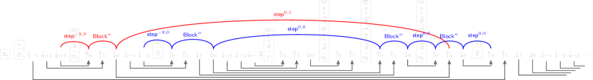
Example 6.4.

The nested-word encoding of the run from Figure 1 is depicted in Figure 2. It is 2-recency bounded. The indices 0 and 1 refer to the most recent and second most recent elements. Negative indices refer to freshly added elements.

Notice that in this example $B_{1}$ is the only block where $|\textsf{Recent}_{\mathbf{b}}(I)|<\mathbf{b}=2$. On all successive blocks $|\textsf{Recent}_{\mathbf{b}}(I)|=2$. In block $B_{1}$, indices 0 and 1 are not used.

In block $B_{2}$, the substitution uses only the second-most recent element, denoted by $u\mapsto 1$. However, the entire $\textsf{Recent}_{\mathbf{b}}(I)$ is popped. Since the second-most recent element is deleted in $B_{2}$, it is not pushed back, but the most recent element is pushed back (denoted by $\downarrow_{0}$). Hence for $B_{2}$, we have $J_{2}=\{0\}$.

Action $\alpha$ of block $B_{3}$ does not use/modify any element from $\textsf{Recent}_{\mathbf{b}}(I)$. However, since $\textsf{Recent}_{\mathbf{b}}(I)$ is non-empty, it is popped entirely and pushed back. Notice the inversion in the order of the sequence of pops and that of pushes. This inversion maintains that less-recent elements are pushed before the more-recent elements.

Notice also that the number of pushes on the left of a block which are not matched on the left correspond to the number of elements in the active domain before the execution of the block. For example, the database instance $I_{4}$ just before the execution of block $B_{5}$ has 6 elements, and the $\textsc{adom}(I_{7})$ has just two elements.

Notice that the abstract substitution need not be injective (cf. block $B_{7}$), and need not assign recent values to variables in the order of their recency (cf. blocks $B_{5}$ and $B_{6}$).

Notice also that the set $J$ is not determined by the action name nor the abstract substitution $s$.

Figure 3: The relation $\textsf{Eq}^{i,j}$ tracks the occurrences of the same element in the nested word encoding of a run. In a way it is a transitive closure of the relations and the $\textsf{Block}^{=}$ relations. Note that if such a transitive closure path enters a block via the relation and exits the block via then $j=i^{\prime}$.

$\textsf{Eq}^{i,j}(x,y)\equiv\\ \forall X_{-\mathbf{\eta}}\forall X_{-\mathbf{\eta}+1}\dots\forall X_{\mathbf{b}-1}\left(\left(x\in X_{i}\wedge\forall x_{1}\forall x_{2}.\left(\begin{array}[]{l}\bigwedge_{\mathbf{\eta}\leq\ell,m\leq\mathbf{b}-1}(\step{}^{\ell,m}(x_{1},x_{2})\wedge{x_{1}\in X_{\ell}})\Rightarrow{x_{2}\in X_{m}}\\ \wedge\bigwedge_{-\mathbf{\eta}\leq\ell\leq\mathbf{b}-1}(\textsf{Block}^{=}(x_{1},x_{2})\wedge{x_{1}\in X_{\ell}})\Rightarrow{x_{2}\in X_{\ell}}\\ \end{array}\right)\right)\\ \Rightarrow y\in X_{j}\right)$

Figure 4: Formula $\textsf{Eq}^{i,j}$ which states that the element indexed by $i$ in the block of the first argument is same as the element indexed by $j$ in the block of the second argument. This is pictorially depicted in Figure 4.

6.3.1 Conditions for valid encodings

Consider any nested word $W$ over the visible alphabet $\Sigma=\Sigma_{\text{int}}\uplus\Sigma_{\uparrow}\uplus\Sigma_{\downarrow}$ of the form $\leavevmode\hbox to18.14pt{\vbox to11.04pt{\pgfpicture\makeatletter\hbox{\hskip 9.07138pt\lower-5.51888pt\hbox to0.0pt{\pgfsys@beginscope\pgfsys@invoke{ }\definecolor{pgfstrokecolor}{rgb}{0,0,0}\pgfsys@color@rgb@stroke{0}{0}{0}\pgfsys@invoke{ }\pgfsys@color@rgb@fill{0}{0}{0}\pgfsys@invoke{ }\pgfsys@setlinewidth{0.4pt}\pgfsys@invoke{ }\nullfont\pgfsys@beginscope\pgfsys@invoke{ }\pgfsys@invoke{\lxSVG@closescope }\pgfsys@endscope\hbox to0.0pt{\pgfsys@beginscope\pgfsys@invoke{ } {{}}\hbox{\hbox{{\pgfsys@beginscope\pgfsys@invoke{ }\definecolor[named]{pgffillcolor}{rgb}{1,1,1}\pgfsys@color@gray@fill{1}\pgfsys@invoke{ }{{}{}{}{}{}{}{}{}{}{}{}{}{}{}{}{}{}{{}}{}{{{}}{}{}{{{{}{}{}{}}}{{}{}{}{}}}{}{{{{}{}{}{}}}{{}{}{}{}}}}{\pgfsys@beginscope\pgfsys@invoke{ }\definecolor[named]{pgffillcolor}{rgb}{1,1,1}\pgfsys@color@gray@fill{1}\pgfsys@invoke{ }{}\pgfsys@moveto{0.0pt}{5.31888pt}\pgfsys@lineto{3.5525pt}{5.31888pt}\pgfsys@curveto{6.49007pt}{5.31888pt}{8.87138pt}{2.93756pt}{8.87138pt}{0.0pt}\pgfsys@curveto{8.87138pt}{-2.93756pt}{6.49007pt}{-5.31888pt}{3.5525pt}{-5.31888pt}\pgfsys@lineto{-3.5525pt}{-5.31888pt}\pgfsys@curveto{-6.49007pt}{-5.31888pt}{-8.87138pt}{-2.93756pt}{-8.87138pt}{0.0pt}\pgfsys@curveto{-8.87138pt}{2.93756pt}{-6.49007pt}{5.31888pt}{-3.5525pt}{5.31888pt}\pgfsys@closepath\pgfsys@fillstroke\pgfsys@invoke{ } \pgfsys@invoke{\lxSVG@closescope }\pgfsys@endscope}{{{{}}\pgfsys@beginscope\pgfsys@invoke{ }\pgfsys@transformcm{1.0}{0.0}{0.0}{1.0}{-5.65694pt}{-2.51443pt}\pgfsys@invoke{ }\hbox{{\definecolor{pgfstrokecolor}{rgb}{0,0,0}\pgfsys@color@rgb@stroke{0}{0}{0}\pgfsys@invoke{ }\pgfsys@color@rgb@fill{0}{0}{0}\pgfsys@invoke{ }\hbox{{$I_{0}$ }} }}\pgfsys@invoke{\lxSVG@closescope }\pgfsys@endscope}}} \pgfsys@invoke{\lxSVG@closescope }\pgfsys@endscope}}} \pgfsys@invoke{\lxSVG@closescope }\pgfsys@endscope{{{}}}{}{}\hss}\pgfsys@discardpath\pgfsys@invoke{\lxSVG@closescope }\pgfsys@endscope\hss}}\lxSVG@closescope\endpgfpicture}}\,\textsf{block}(\alpha_{1},s_{1},m_{1},J_{1})\,\textsf{block}(\alpha_{2},s_{2},m_{2},J_{2})\,\ldots$. Let $w\in(\textsf{symAlph}_{\mathcal{S},\mathbf{b}})^{\omega}$ be obtained by the $\Sigma_{\text{int}}$ projection of $W$. Let $W_{i}$ denote the prefix of $W$ upto $\textsf{block}_{i}$, and $w_{i}$ be the corresponding projection.

For $i\geq 0$, we say that a prefix $W_{i+1}$ is good if $\textsf{Concr}(w_{i})$ is defined. Let $C_{i}=\langle I_{i},H_{i},\texttt{seq\_no}_{i}\rangle$ be the last configuration of $\textsf{Concr}(w_{i})$ in this case. Further we require the following:

1. $m_{i+1}=|\textsf{Recent}_{\mathbf{b}}(I_{i},\texttt{seq\_no}_{i})|$;

2. $j\in J_{i}$ iff, letting $e$ be the element of recency-index $j$ in $C_{i}$, there are a relation $R\in\mathcal{R}$ and a tuple $t$ of $R$ involving $e$ such that $t$ is present in $I_{i}$ but not in instantiated $\alpha_{i+1}{\cdot}\mathit{Del}$, or $t$ is present in instantiated $\alpha_{i+1}{\cdot}\mathit{Add}$; and

3. letting $\sigma_{i+1}$ be the instantiation of $s_{i+1}$ at $C_{i}$, we have $I_{i},\sigma_{i+1}\models\alpha_{i+1}{\cdot}\textsf{guard}$.

We say $W$ is a valid encoding of a $\mathbf{b}$-recency bounded run of $\mathcal{S}$ if $W_{i}$ is good for every $i\geq 0$.

Observe that, if $W_{i}$ is good then $\textsf{Concr}(w_{i})$ is defined. Hence, if a nested word is not a valid encoding, it can be detected at the first index $i$ such that $W_{i}$ is not good by observing that conditions (1), (2) or (3) is violated. In this case $\textsf{Concr}(w_{i-1})$ is defined since $W_{i-1}$ is good. We will exploit this observation to express valid encodings in $\texttt{MSO}_{\texttt{NW}}$.

In the remainder of this section we will use the above-set indexing convention for the intuitive explanations. That is, $C_{i}=\langle I_{i},H_{i},\texttt{seq\_no}_{i}\rangle$ is the last configuration of $\textsf{Concr}(w_{i})$. This means that the previous configuration of $\textsf{block}_{i}$ (or the configuration where it is being executed) is $C_{i-1}$.

Remark 6.12.

If $W$ is a valid encoding then, the number of unmatched pushes in the prefix upto $\textsf{block}_{j+1}$ (excluding) is $|\textsc{adom}(I_{j})|$. The set $\textsf{Recent}_{\mathbf{b}}(I_{j},\texttt{seq\_no}_{j})$ corresponds to the innermost (rightmost) $|\textsf{Recent}_{\mathbf{b}}(I_{j},\texttt{seq\_no}_{j})|$ unmatched pushes in the prefix. Note that, here an unmatched push in the prefix means it is not matched within the prefix; it may be matched after the prefix.

We will now provide $\texttt{MSO}_{\texttt{NW}}$ formulae stating that these three conditions are satisfied by a nested word over $\Sigma$ at all of its blocks. The conjunction of the these formulae will characterise $\textsf{Runs}_{\mathbf{b}}(\mathcal{S})$ (which we denote by $\varphi_{\mathbf{b},\mathcal{S}}^{\textsf{valid}}$).

6.4 Expressing valid encodings in $\texttt{MSO}_{\texttt{NW}}$

We first describe a few $\texttt{MSO}_{\texttt{NW}}$ predicates that turn out handy when stating the validity of an encoding in MSO. Such predicates are macros/abbreviation helping towards the readability of the formula describing validity.

6.4.1 Preliminary formulae

We write $\Sigma_{\text{int}}(x)$ as a shorthand for $\bigvee_{a\in\Sigma_{\text{int}}}a(x)$. Similarly we define $\Sigma_{\downarrow}(x)\equiv\bigvee_{a\in\Sigma_{\downarrow}}a(x)$ and $\Sigma_{\uparrow}(x)\equiv\bigvee_{a\in\Sigma_{\uparrow}}a(x)$.

We write $\textsf{Block}^{=}(x,y)$ to indicate that positions $x$ and $y$ belong to the same block. This is a shorthand for

$$\forall z.\,((\neg\Sigma_{\text{int}}(z))\lor(z\leq x\wedge z\leq y)\vee(x<z\wedge y<z))$$

Notice that a block has exactly one internal letter, which indicates the action and the abstract substitution. The position labelled by such an internal letter is called head, and every block has a unique head. The formula $\textsf{Block}^{=}(x,y)$ says that $x$ and $y$ must not be separated by an internal letter (or a head).

We now define a unary predicate with a free variable $x$ for each relation name $R/a\in\mathcal{R}$ and choice of $a$ recency indices $i_{1},\dotsc i_{a}\in\{0,\ldots,\mathbf{b}-1\}$. The predicate holds at a position if it is the head of a block and its block deletes a tuple $\left\langle{e_{1},\ldots e_{a}}\right\rangle$ from the relation $R$ where $e_{j}$ is indexed by $i_{j}$ in its block, for all $j:1\leq j\leq a$. This predicate is denoted $\mathit{Del}(R(i_{1},\ldots i_{a}))@x$.

$$\mathit{Del}(R(i_{1},\ldots i_{a}))@x\equiv\bigvee_{\leavevmode\hbox to16.62pt{\vbox to10.36pt{\pgfpicture\makeatletter\hbox{\hskip 8.30803pt\lower-5.17923pt\hbox to0.0pt{\pgfsys@beginscope\pgfsys@invoke{ }\definecolor{pgfstrokecolor}{rgb}{0,0,0}\pgfsys@color@rgb@stroke{0}{0}{0}\pgfsys@invoke{ }\pgfsys@color@rgb@fill{0}{0}{0}\pgfsys@invoke{ }\pgfsys@setlinewidth{0.4pt}\pgfsys@invoke{ }\nullfont\pgfsys@beginscope\pgfsys@invoke{ }\pgfsys@invoke{\lxSVG@closescope }\pgfsys@endscope\hbox to0.0pt{\pgfsys@beginscope\pgfsys@invoke{ } {{}}\hbox{\hbox{{\pgfsys@beginscope\pgfsys@invoke{ }\definecolor[named]{pgffillcolor}{rgb}{1,1,1}\pgfsys@color@gray@fill{1}\pgfsys@invoke{ }{{}{}{}{}{}{}{}{}{}{}{}{}{}{}{}{}{}{{}}{}{{{}}{}{}{{{{}{}{}{}}}{{}{}{}{}}}{}{{{{}{}{}{}}}{{}{}{}{}}}}{\pgfsys@beginscope\pgfsys@invoke{ }\definecolor[named]{pgffillcolor}{rgb}{1,1,1}\pgfsys@color@gray@fill{1}\pgfsys@invoke{ }{}\pgfsys@moveto{0.0pt}{4.97923pt}\pgfsys@lineto{3.1288pt}{4.97923pt}\pgfsys@curveto{5.87878pt}{4.97923pt}{8.10803pt}{2.74998pt}{8.10803pt}{0.0pt}\pgfsys@curveto{8.10803pt}{-2.74998pt}{5.87878pt}{-4.97923pt}{3.1288pt}{-4.97923pt}\pgfsys@lineto{-3.1288pt}{-4.97923pt}\pgfsys@curveto{-5.87878pt}{-4.97923pt}{-8.10803pt}{-2.74998pt}{-8.10803pt}{0.0pt}\pgfsys@curveto{-8.10803pt}{2.74998pt}{-5.87878pt}{4.97923pt}{-3.1288pt}{4.97923pt}\pgfsys@closepath\pgfsys@fillstroke\pgfsys@invoke{ } \pgfsys@invoke{\lxSVG@closescope }\pgfsys@endscope}{{{{}}\pgfsys@beginscope\pgfsys@invoke{ }\pgfsys@transformcm{1.0}{0.0}{0.0}{1.0}{-6.60179pt}{-0.8264pt}\pgfsys@invoke{ }\hbox{{\definecolor{pgfstrokecolor}{rgb}{0,0,0}\pgfsys@color@rgb@stroke{0}{0}{0}\pgfsys@invoke{ }\pgfsys@color@rgb@fill{0}{0}{0}\pgfsys@invoke{ }\hbox{{$\alpha,s$ }} }}\pgfsys@invoke{\lxSVG@closescope }\pgfsys@endscope}}} \pgfsys@invoke{\lxSVG@closescope }\pgfsys@endscope}}} \pgfsys@invoke{\lxSVG@closescope }\pgfsys@endscope{{{}}}{}{}\hss}\pgfsys@discardpath\pgfsys@invoke{\lxSVG@closescope }\pgfsys@endscope\hss}}\lxSVG@closescope\endpgfpicture}}\in\Gamma}\leavevmode\hbox to23.47pt{\vbox to10.36pt{\pgfpicture\makeatletter\hbox{\hskip 11.73386pt\lower-5.17923pt\hbox to0.0pt{\pgfsys@beginscope\pgfsys@invoke{ }\definecolor{pgfstrokecolor}{rgb}{0,0,0}\pgfsys@color@rgb@stroke{0}{0}{0}\pgfsys@invoke{ }\pgfsys@color@rgb@fill{0}{0}{0}\pgfsys@invoke{ }\pgfsys@setlinewidth{0.4pt}\pgfsys@invoke{ }\nullfont\pgfsys@beginscope\pgfsys@invoke{ }\pgfsys@invoke{\lxSVG@closescope }\pgfsys@endscope\hbox to0.0pt{\pgfsys@beginscope\pgfsys@invoke{ } {{}}\hbox{\hbox{{\pgfsys@beginscope\pgfsys@invoke{ }\definecolor[named]{pgffillcolor}{rgb}{1,1,1}\pgfsys@color@gray@fill{1}\pgfsys@invoke{ }{{}{}{}{}{}{}{}{}{}{}{}{}{}{}{}{}{}{{}}{}{{{}}{}{}{{{{}{}{}{}}}{{}{}{}{}}}{}{{{{}{}{}{}}}{{}{}{}{}}}}{\pgfsys@beginscope\pgfsys@invoke{ }\definecolor[named]{pgffillcolor}{rgb}{1,1,1}\pgfsys@color@gray@fill{1}\pgfsys@invoke{ }{}\pgfsys@moveto{0.0pt}{4.97923pt}\pgfsys@lineto{6.55463pt}{4.97923pt}\pgfsys@curveto{9.30461pt}{4.97923pt}{11.53386pt}{2.74998pt}{11.53386pt}{0.0pt}\pgfsys@curveto{11.53386pt}{-2.74998pt}{9.30461pt}{-4.97923pt}{6.55463pt}{-4.97923pt}\pgfsys@lineto{-6.55463pt}{-4.97923pt}\pgfsys@curveto{-9.30461pt}{-4.97923pt}{-11.53386pt}{-2.74998pt}{-11.53386pt}{0.0pt}\pgfsys@curveto{-11.53386pt}{2.74998pt}{-9.30461pt}{4.97923pt}{-6.55463pt}{4.97923pt}\pgfsys@closepath\pgfsys@fillstroke\pgfsys@invoke{ } \pgfsys@invoke{\lxSVG@closescope }\pgfsys@endscope}{{{{}}\pgfsys@beginscope\pgfsys@invoke{ }\pgfsys@transformcm{1.0}{0.0}{0.0}{1.0}{-9.43112pt}{-1.18056pt}\pgfsys@invoke{ }\hbox{{\definecolor{pgfstrokecolor}{rgb}{0,0,0}\pgfsys@color@rgb@stroke{0}{0}{0}\pgfsys@invoke{ }\pgfsys@color@rgb@fill{0}{0}{0}\pgfsys@invoke{ }\hbox{{$\alpha,s$ }} }}\pgfsys@invoke{\lxSVG@closescope }\pgfsys@endscope}}} \pgfsys@invoke{\lxSVG@closescope }\pgfsys@endscope}}} \pgfsys@invoke{\lxSVG@closescope }\pgfsys@endscope{{{}}}{}{}\hss}\pgfsys@discardpath\pgfsys@invoke{\lxSVG@closescope }\pgfsys@endscope\hss}}\lxSVG@closescope\endpgfpicture}}(x) \alpha,s \alpha,s \alpha,s \alpha,s$$

where $\Gamma=\{~{}\leavevmode\hbox to23.47pt{\vbox to10.36pt{\pgfpicture\makeatletter\hbox{\hskip 11.73386pt\lower-5.17923pt\hbox to0.0pt{\pgfsys@beginscope\pgfsys@invoke{ }\definecolor{pgfstrokecolor}{rgb}{0,0,0}\pgfsys@color@rgb@stroke{0}{0}{0}\pgfsys@invoke{ }\pgfsys@color@rgb@fill{0}{0}{0}\pgfsys@invoke{ }\pgfsys@setlinewidth{0.4pt}\pgfsys@invoke{ }\nullfont\pgfsys@beginscope\pgfsys@invoke{ }\pgfsys@invoke{\lxSVG@closescope }\pgfsys@endscope\hbox to0.0pt{\pgfsys@beginscope\pgfsys@invoke{ } {{}}\hbox{\hbox{{\pgfsys@beginscope\pgfsys@invoke{ }\definecolor[named]{pgffillcolor}{rgb}{1,1,1}\pgfsys@color@gray@fill{1}\pgfsys@invoke{ }{{}{}{}{}{}{}{}{}{}{}{}{}{}{}{}{}{}{{}}{}{{{}}{}{}{{{{}{}{}{}}}{{}{}{}{}}}{}{{{{}{}{}{}}}{{}{}{}{}}}}{\pgfsys@beginscope\pgfsys@invoke{ }\definecolor[named]{pgffillcolor}{rgb}{1,1,1}\pgfsys@color@gray@fill{1}\pgfsys@invoke{ }{}\pgfsys@moveto{0.0pt}{4.97923pt}\pgfsys@lineto{6.55463pt}{4.97923pt}\pgfsys@curveto{9.30461pt}{4.97923pt}{11.53386pt}{2.74998pt}{11.53386pt}{0.0pt}\pgfsys@curveto{11.53386pt}{-2.74998pt}{9.30461pt}{-4.97923pt}{6.55463pt}{-4.97923pt}\pgfsys@lineto{-6.55463pt}{-4.97923pt}\pgfsys@curveto{-9.30461pt}{-4.97923pt}{-11.53386pt}{-2.74998pt}{-11.53386pt}{0.0pt}\pgfsys@curveto{-11.53386pt}{2.74998pt}{-9.30461pt}{4.97923pt}{-6.55463pt}{4.97923pt}\pgfsys@closepath\pgfsys@fillstroke\pgfsys@invoke{ } \pgfsys@invoke{\lxSVG@closescope }\pgfsys@endscope}{{{{}}\pgfsys@beginscope\pgfsys@invoke{ }\pgfsys@transformcm{1.0}{0.0}{0.0}{1.0}{-9.43112pt}{-1.18056pt}\pgfsys@invoke{ }\hbox{{\definecolor{pgfstrokecolor}{rgb}{0,0,0}\pgfsys@color@rgb@stroke{0}{0}{0}\pgfsys@invoke{ }\pgfsys@color@rgb@fill{0}{0}{0}\pgfsys@invoke{ }\hbox{{$\alpha,s$ }} }}\pgfsys@invoke{\lxSVG@closescope }\pgfsys@endscope}}} \pgfsys@invoke{\lxSVG@closescope }\pgfsys@endscope}}} \pgfsys@invoke{\lxSVG@closescope }\pgfsys@endscope{{{}}}{}{}\hss}\pgfsys@discardpath\pgfsys@invoke{\lxSVG@closescope }\pgfsys@endscope\hss}}\lxSVG@closescope\endpgfpicture}}\mid\alpha{\cdot}\mathit{Del}$ contains a tuple $R(u_{1}\ldots u_{a})$ and $s(u_{j})=i_{j}$ for all $1\leq j\leq a\}$.

Similarly we define a unary predicate for adding a tuple to a relation as well. However in this case, the indices may refer to the fresh data values as well. Hence we have unary predicate $\mathit{Add}(R(i_{1},\ldots i_{a}))@x$ for each relation name $R/a\in\mathcal{R}$ and choice of $a$ indices $i_{1},\dotsc i_{a}\in\{-n,\ldots,0,\ldots,\mathbf{b}-1\}$, where $n:=\max_{\alpha\in\textsc{acts}}{|\alpha{\cdot}\textsf{new}|}$.

$$\mathit{Add}(R(i_{1},\ldots i_{a}))@x\equiv\bigvee_{\leavevmode\hbox to16.62pt{\vbox to10.36pt{\pgfpicture\makeatletter\hbox{\hskip 8.30803pt\lower-5.17923pt\hbox to0.0pt{\pgfsys@beginscope\pgfsys@invoke{ }\definecolor{pgfstrokecolor}{rgb}{0,0,0}\pgfsys@color@rgb@stroke{0}{0}{0}\pgfsys@invoke{ }\pgfsys@color@rgb@fill{0}{0}{0}\pgfsys@invoke{ }\pgfsys@setlinewidth{0.4pt}\pgfsys@invoke{ }\nullfont\pgfsys@beginscope\pgfsys@invoke{ }\pgfsys@invoke{\lxSVG@closescope }\pgfsys@endscope\hbox to0.0pt{\pgfsys@beginscope\pgfsys@invoke{ } {{}}\hbox{\hbox{{\pgfsys@beginscope\pgfsys@invoke{ }\definecolor[named]{pgffillcolor}{rgb}{1,1,1}\pgfsys@color@gray@fill{1}\pgfsys@invoke{ }{{}{}{}{}{}{}{}{}{}{}{}{}{}{}{}{}{}{{}}{}{{{}}{}{}{{{{}{}{}{}}}{{}{}{}{}}}{}{{{{}{}{}{}}}{{}{}{}{}}}}{\pgfsys@beginscope\pgfsys@invoke{ }\definecolor[named]{pgffillcolor}{rgb}{1,1,1}\pgfsys@color@gray@fill{1}\pgfsys@invoke{ }{}\pgfsys@moveto{0.0pt}{4.97923pt}\pgfsys@lineto{3.1288pt}{4.97923pt}\pgfsys@curveto{5.87878pt}{4.97923pt}{8.10803pt}{2.74998pt}{8.10803pt}{0.0pt}\pgfsys@curveto{8.10803pt}{-2.74998pt}{5.87878pt}{-4.97923pt}{3.1288pt}{-4.97923pt}\pgfsys@lineto{-3.1288pt}{-4.97923pt}\pgfsys@curveto{-5.87878pt}{-4.97923pt}{-8.10803pt}{-2.74998pt}{-8.10803pt}{0.0pt}\pgfsys@curveto{-8.10803pt}{2.74998pt}{-5.87878pt}{4.97923pt}{-3.1288pt}{4.97923pt}\pgfsys@closepath\pgfsys@fillstroke\pgfsys@invoke{ } \pgfsys@invoke{\lxSVG@closescope }\pgfsys@endscope}{{{{}}\pgfsys@beginscope\pgfsys@invoke{ }\pgfsys@transformcm{1.0}{0.0}{0.0}{1.0}{-6.60179pt}{-0.8264pt}\pgfsys@invoke{ }\hbox{{\definecolor{pgfstrokecolor}{rgb}{0,0,0}\pgfsys@color@rgb@stroke{0}{0}{0}\pgfsys@invoke{ }\pgfsys@color@rgb@fill{0}{0}{0}\pgfsys@invoke{ }\hbox{{$\alpha,s$ }} }}\pgfsys@invoke{\lxSVG@closescope }\pgfsys@endscope}}} \pgfsys@invoke{\lxSVG@closescope }\pgfsys@endscope}}} \pgfsys@invoke{\lxSVG@closescope }\pgfsys@endscope{{{}}}{}{}\hss}\pgfsys@discardpath\pgfsys@invoke{\lxSVG@closescope }\pgfsys@endscope\hss}}\lxSVG@closescope\endpgfpicture}}\in\Gamma}\leavevmode\hbox to23.47pt{\vbox to10.36pt{\pgfpicture\makeatletter\hbox{\hskip 11.73386pt\lower-5.17923pt\hbox to0.0pt{\pgfsys@beginscope\pgfsys@invoke{ }\definecolor{pgfstrokecolor}{rgb}{0,0,0}\pgfsys@color@rgb@stroke{0}{0}{0}\pgfsys@invoke{ }\pgfsys@color@rgb@fill{0}{0}{0}\pgfsys@invoke{ }\pgfsys@setlinewidth{0.4pt}\pgfsys@invoke{ }\nullfont\pgfsys@beginscope\pgfsys@invoke{ }\pgfsys@invoke{\lxSVG@closescope }\pgfsys@endscope\hbox to0.0pt{\pgfsys@beginscope\pgfsys@invoke{ } {{}}\hbox{\hbox{{\pgfsys@beginscope\pgfsys@invoke{ }\definecolor[named]{pgffillcolor}{rgb}{1,1,1}\pgfsys@color@gray@fill{1}\pgfsys@invoke{ }{{}{}{}{}{}{}{}{}{}{}{}{}{}{}{}{}{}{{}}{}{{{}}{}{}{{{{}{}{}{}}}{{}{}{}{}}}{}{{{{}{}{}{}}}{{}{}{}{}}}}{\pgfsys@beginscope\pgfsys@invoke{ }\definecolor[named]{pgffillcolor}{rgb}{1,1,1}\pgfsys@color@gray@fill{1}\pgfsys@invoke{ }{}\pgfsys@moveto{0.0pt}{4.97923pt}\pgfsys@lineto{6.55463pt}{4.97923pt}\pgfsys@curveto{9.30461pt}{4.97923pt}{11.53386pt}{2.74998pt}{11.53386pt}{0.0pt}\pgfsys@curveto{11.53386pt}{-2.74998pt}{9.30461pt}{-4.97923pt}{6.55463pt}{-4.97923pt}\pgfsys@lineto{-6.55463pt}{-4.97923pt}\pgfsys@curveto{-9.30461pt}{-4.97923pt}{-11.53386pt}{-2.74998pt}{-11.53386pt}{0.0pt}\pgfsys@curveto{-11.53386pt}{2.74998pt}{-9.30461pt}{4.97923pt}{-6.55463pt}{4.97923pt}\pgfsys@closepath\pgfsys@fillstroke\pgfsys@invoke{ } \pgfsys@invoke{\lxSVG@closescope }\pgfsys@endscope}{{{{}}\pgfsys@beginscope\pgfsys@invoke{ }\pgfsys@transformcm{1.0}{0.0}{0.0}{1.0}{-9.43112pt}{-1.18056pt}\pgfsys@invoke{ }\hbox{{\definecolor{pgfstrokecolor}{rgb}{0,0,0}\pgfsys@color@rgb@stroke{0}{0}{0}\pgfsys@invoke{ }\pgfsys@color@rgb@fill{0}{0}{0}\pgfsys@invoke{ }\hbox{{$\alpha,s$ }} }}\pgfsys@invoke{\lxSVG@closescope }\pgfsys@endscope}}} \pgfsys@invoke{\lxSVG@closescope }\pgfsys@endscope}}} \pgfsys@invoke{\lxSVG@closescope }\pgfsys@endscope{{{}}}{}{}\hss}\pgfsys@discardpath\pgfsys@invoke{\lxSVG@closescope }\pgfsys@endscope\hss}}\lxSVG@closescope\endpgfpicture}}(x) \alpha,s \alpha,s \alpha,s \alpha,s$$

where $\Gamma=\{~{}\leavevmode\hbox to23.47pt{\vbox to10.36pt{\pgfpicture\makeatletter\hbox{\hskip 11.73386pt\lower-5.17923pt\hbox to0.0pt{\pgfsys@beginscope\pgfsys@invoke{ }\definecolor{pgfstrokecolor}{rgb}{0,0,0}\pgfsys@color@rgb@stroke{0}{0}{0}\pgfsys@invoke{ }\pgfsys@color@rgb@fill{0}{0}{0}\pgfsys@invoke{ }\pgfsys@setlinewidth{0.4pt}\pgfsys@invoke{ }\nullfont\pgfsys@beginscope\pgfsys@invoke{ }\pgfsys@invoke{\lxSVG@closescope }\pgfsys@endscope\hbox to0.0pt{\pgfsys@beginscope\pgfsys@invoke{ } {{}}\hbox{\hbox{{\pgfsys@beginscope\pgfsys@invoke{ }\definecolor[named]{pgffillcolor}{rgb}{1,1,1}\pgfsys@color@gray@fill{1}\pgfsys@invoke{ }{{}{}{}{}{}{}{}{}{}{}{}{}{}{}{}{}{}{{}}{}{{{}}{}{}{{{{}{}{}{}}}{{}{}{}{}}}{}{{{{}{}{}{}}}{{}{}{}{}}}}{\pgfsys@beginscope\pgfsys@invoke{ }\definecolor[named]{pgffillcolor}{rgb}{1,1,1}\pgfsys@color@gray@fill{1}\pgfsys@invoke{ }{}\pgfsys@moveto{0.0pt}{4.97923pt}\pgfsys@lineto{6.55463pt}{4.97923pt}\pgfsys@curveto{9.30461pt}{4.97923pt}{11.53386pt}{2.74998pt}{11.53386pt}{0.0pt}\pgfsys@curveto{11.53386pt}{-2.74998pt}{9.30461pt}{-4.97923pt}{6.55463pt}{-4.97923pt}\pgfsys@lineto{-6.55463pt}{-4.97923pt}\pgfsys@curveto{-9.30461pt}{-4.97923pt}{-11.53386pt}{-2.74998pt}{-11.53386pt}{0.0pt}\pgfsys@curveto{-11.53386pt}{2.74998pt}{-9.30461pt}{4.97923pt}{-6.55463pt}{4.97923pt}\pgfsys@closepath\pgfsys@fillstroke\pgfsys@invoke{ } \pgfsys@invoke{\lxSVG@closescope }\pgfsys@endscope}{{{{}}\pgfsys@beginscope\pgfsys@invoke{ }\pgfsys@transformcm{1.0}{0.0}{0.0}{1.0}{-9.43112pt}{-1.18056pt}\pgfsys@invoke{ }\hbox{{\definecolor{pgfstrokecolor}{rgb}{0,0,0}\pgfsys@color@rgb@stroke{0}{0}{0}\pgfsys@invoke{ }\pgfsys@color@rgb@fill{0}{0}{0}\pgfsys@invoke{ }\hbox{{$\alpha,s$ }} }}\pgfsys@invoke{\lxSVG@closescope }\pgfsys@endscope}}} \pgfsys@invoke{\lxSVG@closescope }\pgfsys@endscope}}} \pgfsys@invoke{\lxSVG@closescope }\pgfsys@endscope{{{}}}{}{}\hss}\pgfsys@discardpath\pgfsys@invoke{\lxSVG@closescope }\pgfsys@endscope\hss}}\lxSVG@closescope\endpgfpicture}}\mid\alpha{\cdot}\mathit{Add}$ contains a tuple $R(\xi_{1}\ldots\xi_{a})$ and for all $1\leq j\leq a$ if $\xi_{j}\in\alpha{\cdot}\textsf{free}$ then $s(\xi_{j})=i_{j}$ and if $\xi_{j}$ is the $k$th fresh input variable $v_{k}$ then $i_{j}=-k\}$.

Equality between indexed elements of different blocks. Consider the encoding of the run in Figure 2. Notice that the index $-2$ in the block $B_{1}$ and index $1$ in the block $B_{2}$ refer to the same element ($e_{2}$ in the concrete run of Figure 1). Notice also that the element referred to by index $-2$ in Block $B_{2}$ is the same as the element referred to by index $0$ in block $B_{7}$ ($e_{5}$ in the concrete run of Figure 1).

Given two positions $x$ and $y$ and indices $i$ and $j$, consider following question: Is the element referred to by index $i$ in the block of $x$ the same as the element referred to by index $j$ in the block of $y$? In fact, this property can be expressed in $\texttt{MSO}_{\texttt{NW}}$. We define below a binary predicate $\textsf{Eq}^{i,j}(x,y)$ for the same. Indeed we will define such a predicate for every pair $i,j$ with $-\mathbf{\eta}\leq i,j\leq\mathbf{b}-1$.

Towards this, first notice that the predicate must hold if there is a $\downarrow_{i}$-labelled position in the block of $x$ that is $\triangleright$-related to $\uparrow_{j}$-labelled position in the block of $y$. This forms the basic step relation towards defining $\textsf{Eq}^{i,j}(x,y)$.

$$\exists z_{1}\exists z_{2}.\textsf{Block}^{=}(z_{1},x)\wedge\textsf{Block}^{=}(z_{2},y)$$

$$\wedge z_{1}\triangleright z_{2}\wedge{\downarrow_{i}}(z_{1})\wedge{\uparrow_{j}}(z_{2})$$

Recall that ${\downarrow_{i}}(x)$ means that the position $x$ is labelled by the letter $\downarrow_{i}$. Notice that our definition of is directional, in the sense that $x$ must necessarily be before $y$ for to hold. The transitive closure of the above relation gives us the required predicate $\textsf{Eq}^{i,j}(x,y)$. Suppose the element indexed $i$ in the block of $x$ is $e$. The element $e$ may appear with different indices at the intermediate steps. Hence we need to take a zig-zag transitive closure. Our formula uses $\mathbf{b}+\mathbf{\eta}$ second-order position variables. Intuitively the set $X_{k}$ contains the set of positions such that the element $e$ is indexed by $k$ in its block. Using the universal quantifier, we require that the minimal of such sets which are closed under the zig-zag transitive closure must contain $y$ in the set $X_{j}$. The formula $\textsf{Eq}^{i,j}(x,y)$ is depicted in Figure 4.

Notice that since is directional, so is $\textsf{Eq}^{i,j}(x,y)$. I.e, if $\textsf{Eq}^{i,j}(x,y)$ then necessarily $x\leq y$ or $\textsf{Block}^{=}(x,y)$.

Recent elements participating in a relation. Consider a relation $R$ of arity $a$. We define a predicate $\textsf{Rel-R}(x_{1},i_{1},x_{2},i_{2},\dots x_{a},i_{a})@y^{\circleddash}$ which holds iff the database instance before the execution of the block of $y$ has the tuple $\langle e_{1},e_{2},\dotsc e_{a}\rangle$ in relation $R$ where, the element $e_{j}$ is indexed by $i_{j}$ in the block of $x_{j}$ for all $j:1\leq j\leq a$. This predicate can be expressed in MSO, as given below.

$$\exists x\,x<y\wedge\neg\textsf{Block}^{=}(x,y)\wedge$$

$$\bigvee_{-\mathbf{\eta}\leq\ell_{1},\ldots\ell_{a}\leq\mathbf{b}-1}\,\mathit{Add}(R(\ell_{1},\ldots\ell_{a})@x)\wedge\bigwedge_{1\leq j\leq a}\textsf{Eq}^{\ell_{j},i_{j}}(x,x_{j})$$

$$\wedge\forall z\,\neg{\color[rgb]{1,0,0}\definecolor[named]{pgfstrokecolor}{rgb}{1,0,0}(}x\leq z\wedge z<y\wedge\neg\textsf{Block}^{=}(z,y)\wedge$$

$$\bigvee_{0\leq m_{1},\ldots m_{a}\leq\mathbf{b}-1}{\color[rgb]{0,0,1}\definecolor[named]{pgfstrokecolor}{rgb}{0,0,1}(}\mathit{Del}(R(m_{1},\ldots m_{a}))@z\wedge\bigwedge_{1\leq j\leq a}\textsf{Eq}^{\ell_{j},m_{j}}(x,z){\color[rgb]{0,0,1}\definecolor[named]{pgfstrokecolor}{rgb}{0,0,1})}{\color[rgb]{1,0,0}\definecolor[named]{pgfstrokecolor}{rgb}{1,0,0})}$$

The formula essentially says that the relation tuple has been added to the database instance at some point in the past of $y$, and since then it has not been deleted.

Similarly we define $\textsf{Rel-R}(x_{1},i_{1},x_{2},i_{2},\dots x_{n},i_{n})@y^{\oplus}$ which holds iff the database instance after the execution of the block of $y$ has a tuple in relation $R$ as before. It can be expressed as given follows:

$$\exists x\,x\leq y\wedge\bigvee_{-\mathbf{\eta}\leq\ell_{1},\ldots\ell_{a}\leq\mathbf{b}-1}\,\mathit{Add}(R(\ell_{1},\ldots\ell_{a}))@x\wedge$$

$$\bigwedge_{1\leq j\leq a}\textsf{Eq}^{\ell_{j},i_{j}}(x,x_{j})\wedge\forall z\,\neg{\color[rgb]{1,0,0}\definecolor[named]{pgfstrokecolor}{rgb}{1,0,0}(}x\leq z\wedge z\leq y\wedge$$

$$\bigvee_{0\leq m_{1},\dotsc,m_{a}\leq\mathbf{b}-1}{\color[rgb]{0,0,1}\definecolor[named]{pgfstrokecolor}{rgb}{0,0,1}(}\mathit{Del}(R(m_{1},\ldots m_{a}))@z\wedge\bigwedge_{1\leq j\leq a}\textsf{Eq}^{\ell_{j},m_{j}}(x,z){\color[rgb]{0,0,1}\definecolor[named]{pgfstrokecolor}{rgb}{0,0,1})}{\color[rgb]{1,0,0}\definecolor[named]{pgfstrokecolor}{rgb}{1,0,0})}$$

6.4.2 Expressing valid encodings in $\texttt{MSO}_{\texttt{NW}}$

We now show that the conditions given in Section 6.3.1 can be expressed in $\texttt{MSO}_{\texttt{NW}}$.

0. Well-formedness We need to check the local consistency of each block appearing in the word, which means $s_{i}$ must not assign a variable to a recency index higher than or equal to $m_{i}$, and that $J_{i}\subseteq\{0,\ldots,m_{i}\}$. Further it must of the form described in Section 6.3.1. This is a syntactic check inside a block and can be easily stated in $\texttt{MSO}_{\texttt{NW}}$.

1. Consistency of $m$. We write a formula $\varphi^{\text{Recent}}_{m}(x)$ to state that, just before executing the block of $x$, the current database $I$ has at least $m+1$ elements in $\textsc{adom}(I)$. Thanks to Remark 6.12, this can be expressed in $\texttt{MSO}_{\texttt{NW}}$ by saying that there are $m+1$ distinct pushes before the block of $x$ which are not popped until $x$. $\varphi^{\text{Recent}}_{m}(x)\equiv\exists y\,\textsf{Block}^{=}(x,y)\wedge\Sigma_{\text{int}}(y)\wedge\exists x_{1},\ldots x_{m}$ $\bigwedge_{i\neq j}x_{i}\neq x_{j}\wedge\bigwedge_{i}\big{(}\Sigma_{\downarrow}(x_{i})\wedge x_{i}<y\wedge\forall z(x_{i}\triangleright z\Rightarrow y<z)\big{)}$ Now, consistency of $m$ can be stated as:

$$\forall x\bigwedge_{0\leq i\leq\mathbf{b}-1}\neg\varphi^{\text{Recent}}_{i}(x)\vee\exists y\,({\uparrow_{i}}(y)\wedge\textsf{Block}^{=}(x,y))$$

2. Consistency of J. Towards this we first need to write a formula $\textsf{live}(x,i)$ which holds only if the element with recency index $i$ in the block of $x$ is in $\textsc{adom}(I)$ after the execution of the block of $x$. This is expressed similarly to the formula $\textsf{Active}(u)$ of Example 2.1. $\textsf{live}(x,i)\equiv\bigvee_{R/a\in\mathcal{R}}\,\exists x_{1},\dotsc,x_{a}\bigwedge_{1\leq j\leq a}x_{i}\leq x\wedge\bigvee_{-\mathbf{\eta}\leq i_{1},i_{2},\dotsc,i_{a}\leq\mathbf{b}-1}\,\\ \bigvee_{1\leq j\leq a}\textsf{Rel-R}(\dotsc,x_{j-1},i_{j-1},x,i,x_{j+1},i_{j+1},\dots)@x^{\oplus}$ where $\mathbf{\eta}=\max_{\alpha\in act}|\alpha{\cdot}\textsf{new}|$.

Now the consistency of $J$ can be stated by saying that a recency index is pushed in a block iff it is live:

$$\forall x\bigwedge_{0\leq i\leq\mathbf{b}-1}\textsf{live}(x,i)\Leftrightarrow\big{(}\exists y\,{\downarrow_{i}}(y)\wedge\textsf{Block}^{=}(x,y)\big{)}$$

3. Consistency of action guards. We first present a syntactic translation of an $\mathtt{FOL}(\mathcal{R})$ formula into an $\texttt{MSO}_{\texttt{NW}}$ formula. The translation also depends on the current block (a block is represented by the head position of the block which we denote by a free position variable $x$) as well as the action $\alpha$ and the abstract substitution $s$ used in the block. The translation of an $\mathtt{FOL}(\mathcal{R})$ formula $Q$ at $x$ wrt. $s$ and $\alpha$ is a $\texttt{MSO}_{\texttt{NW}}$ formula denoted $\lfloor{Q}\rfloor_{\alpha,s,x}$.

In our translation, a first-order data variable $u$ is represented by the position $x^{u}$ and an index $i^{u}$, which is an number between $-\mathbf{\eta}$ and $\mathbf{b}-1$ where $\mathbf{\eta}=\max_{\alpha\in\textsc{acts}}|\alpha{\cdot}\textsf{new}|$. Intuitively, instead of reasoning about an element in the domain, we reason about it symbolically by means of a (past) position where it is live and its recency index at that position. Given $\alpha$, $s$ and $x$, we distinguish between variables belonging to $\alpha{\cdot}\textsf{free}$ and the other variables. For a variable $u\in\alpha{\cdot}\textsf{free}$ we set $x^{u}=x$ and $i^{u}=s(u)$.

The translation is defined inductively as follows: (In the following $x^{u}=x$ and $i^{u}=s(u)$ if $u\in\alpha{\cdot}\textsf{free}$, and $\mathbf{\eta}=\max_{\alpha\in\textsc{acts}}|\alpha{\cdot}\textsf{new}|$ )

• $\lfloor{R(u_{1},\ldots u_{n})}\rfloor_{\alpha,s,x}\equiv\textsf{Rel-R}(x^{u_{1}},i^{u_{1}},\ldots,x^{u_{n}},i^{u_{n}})@x^{\circleddash}$

• $\lfloor{u_{1}=u_{2}}\rfloor_{\alpha,s,x}\equiv\textsf{Eq}^{i^{u_{1}},i^{u_{2}}}(x^{u_{1}},x^{u_{2}})$

• $\lfloor{\exists u\ldotp Q}\rfloor_{\alpha,s,x}\equiv\exists x^{u}\ldotp x^{u}<x\wedge\bigvee_{-\mathbf{\eta}\leq i^{u}\leq\mathbf{b}-1}\lfloor{Q}\rfloor_{\alpha,s,x}$

• $\lfloor{Q_{1}\wedge Q_{2}}\rfloor_{\alpha,s,x}\equiv\lfloor{Q_{1}}\rfloor_{\alpha,s,x}\wedge\lfloor{Q_{2}}\rfloor_{\alpha,s,x}$

• $\lfloor{\neg Q}\rfloor_{\alpha,s,x}\equiv\neg\lfloor{Q}\rfloor_{\alpha,s,x}$

Now we are ready to express the consistency of action guards with the run. It can be expressed by the following formula: $\forall x\,\bigwedge_{\leavevmode\hbox to18.79pt{\vbox to10.36pt{\pgfpicture\makeatletter\hbox{\hskip 9.39645pt\lower-5.17923pt\hbox to0.0pt{\pgfsys@beginscope\pgfsys@invoke{ }\definecolor{pgfstrokecolor}{rgb}{0,0,0}\pgfsys@color@rgb@stroke{0}{0}{0}\pgfsys@invoke{ }\pgfsys@color@rgb@fill{0}{0}{0}\pgfsys@invoke{ }\pgfsys@setlinewidth{0.4pt}\pgfsys@invoke{ }\nullfont\pgfsys@beginscope\pgfsys@invoke{ }\pgfsys@invoke{\lxSVG@closescope }\pgfsys@endscope\hbox to0.0pt{\pgfsys@beginscope\pgfsys@invoke{ } {{}}\hbox{\hbox{{\pgfsys@beginscope\pgfsys@invoke{ }\definecolor[named]{pgffillcolor}{rgb}{1,1,1}\pgfsys@color@gray@fill{1}\pgfsys@invoke{ }{{}{}{}{}{}{}{}{}{}{}{}{}{}{}{}{}{}{{}}{}{{{}}{}{}{{{{}{}{}{}}}{{}{}{}{}}}{}{{{{}{}{}{}}}{{}{}{}{}}}}{\pgfsys@beginscope\pgfsys@invoke{ }\definecolor[named]{pgffillcolor}{rgb}{1,1,1}\pgfsys@color@gray@fill{1}\pgfsys@invoke{ }{}\pgfsys@moveto{0.0pt}{4.97923pt}\pgfsys@lineto{4.21722pt}{4.97923pt}\pgfsys@curveto{6.96721pt}{4.97923pt}{9.19646pt}{2.74998pt}{9.19646pt}{0.0pt}\pgfsys@curveto{9.19646pt}{-2.74998pt}{6.96721pt}{-4.97923pt}{4.21722pt}{-4.97923pt}\pgfsys@lineto{-4.21722pt}{-4.97923pt}\pgfsys@curveto{-6.96721pt}{-4.97923pt}{-9.19646pt}{-2.74998pt}{-9.19646pt}{0.0pt}\pgfsys@curveto{-9.19646pt}{2.74998pt}{-6.96721pt}{4.97923pt}{-4.21722pt}{4.97923pt}\pgfsys@closepath\pgfsys@fillstroke\pgfsys@invoke{ } \pgfsys@invoke{\lxSVG@closescope }\pgfsys@endscope}{{{{}}\pgfsys@beginscope\pgfsys@invoke{ }\pgfsys@transformcm{1.0}{0.0}{0.0}{1.0}{-7.96289pt}{-1.50694pt}\pgfsys@invoke{ }\hbox{{\definecolor{pgfstrokecolor}{rgb}{0,0,0}\pgfsys@color@rgb@stroke{0}{0}{0}\pgfsys@invoke{ }\pgfsys@color@rgb@fill{0}{0}{0}\pgfsys@invoke{ }\hbox{{$\alpha:s$ }} }}\pgfsys@invoke{\lxSVG@closescope }\pgfsys@endscope}}} \pgfsys@invoke{\lxSVG@closescope }\pgfsys@endscope}}} \pgfsys@invoke{\lxSVG@closescope }\pgfsys@endscope{{{}}}{}{}\hss}\pgfsys@discardpath\pgfsys@invoke{\lxSVG@closescope }\pgfsys@endscope\hss}}\lxSVG@closescope\endpgfpicture}}\in\Sigma_{\text{int}}}\leavevmode\hbox to23.47pt{\vbox to10.36pt{\pgfpicture\makeatletter\hbox{\hskip 11.73386pt\lower-5.17923pt\hbox to0.0pt{\pgfsys@beginscope\pgfsys@invoke{ }\definecolor{pgfstrokecolor}{rgb}{0,0,0}\pgfsys@color@rgb@stroke{0}{0}{0}\pgfsys@invoke{ }\pgfsys@color@rgb@fill{0}{0}{0}\pgfsys@invoke{ }\pgfsys@setlinewidth{0.4pt}\pgfsys@invoke{ }\nullfont\pgfsys@beginscope\pgfsys@invoke{ }\pgfsys@invoke{\lxSVG@closescope }\pgfsys@endscope\hbox to0.0pt{\pgfsys@beginscope\pgfsys@invoke{ } {{}}\hbox{\hbox{{\pgfsys@beginscope\pgfsys@invoke{ }\definecolor[named]{pgffillcolor}{rgb}{1,1,1}\pgfsys@color@gray@fill{1}\pgfsys@invoke{ }{{}{}{}{}{}{}{}{}{}{}{}{}{}{}{}{}{}{{}}{}{{{}}{}{}{{{{}{}{}{}}}{{}{}{}{}}}{}{{{{}{}{}{}}}{{}{}{}{}}}}{\pgfsys@beginscope\pgfsys@invoke{ }\definecolor[named]{pgffillcolor}{rgb}{1,1,1}\pgfsys@color@gray@fill{1}\pgfsys@invoke{ }{}\pgfsys@moveto{0.0pt}{4.97923pt}\pgfsys@lineto{6.55463pt}{4.97923pt}\pgfsys@curveto{9.30461pt}{4.97923pt}{11.53386pt}{2.74998pt}{11.53386pt}{0.0pt}\pgfsys@curveto{11.53386pt}{-2.74998pt}{9.30461pt}{-4.97923pt}{6.55463pt}{-4.97923pt}\pgfsys@lineto{-6.55463pt}{-4.97923pt}\pgfsys@curveto{-9.30461pt}{-4.97923pt}{-11.53386pt}{-2.74998pt}{-11.53386pt}{0.0pt}\pgfsys@curveto{-11.53386pt}{2.74998pt}{-9.30461pt}{4.97923pt}{-6.55463pt}{4.97923pt}\pgfsys@closepath\pgfsys@fillstroke\pgfsys@invoke{ } \pgfsys@invoke{\lxSVG@closescope }\pgfsys@endscope}{{{{}}\pgfsys@beginscope\pgfsys@invoke{ }\pgfsys@transformcm{1.0}{0.0}{0.0}{1.0}{-9.43112pt}{-1.18056pt}\pgfsys@invoke{ }\hbox{{\definecolor{pgfstrokecolor}{rgb}{0,0,0}\pgfsys@color@rgb@stroke{0}{0}{0}\pgfsys@invoke{ }\pgfsys@color@rgb@fill{0}{0}{0}\pgfsys@invoke{ }\hbox{{$\alpha,s$ }} }}\pgfsys@invoke{\lxSVG@closescope }\pgfsys@endscope}}} \pgfsys@invoke{\lxSVG@closescope }\pgfsys@endscope}}} \pgfsys@invoke{\lxSVG@closescope }\pgfsys@endscope{{{}}}{}{}\hss}\pgfsys@discardpath\pgfsys@invoke{\lxSVG@closescope }\pgfsys@endscope\hss}}\lxSVG@closescope\endpgfpicture}}(x)\Rightarrow\lfloor{\alpha{\cdot}\textsf{guard}}\rfloor_{\alpha,s,x}$.

Let $\varphi_{\mathbf{b},\mathcal{S}}^{\textsf{valid}}$ be the conjunction of the four conditions listed above. It characterises valid encodings of $\mathbf{b}$-bounded runs of a DMS $\mathcal{S}$.

6.5 Translating MSO-FO specifications into $\texttt{MSO}_{\texttt{NW}}$ specifications

Here we provide a translation of the specifications in MSO-FO to an equivalent one in $\texttt{MSO}_{\texttt{NW}}$ over valid encodings of runs. This is similar in spirit to the translation described for action guards. As done there, we represent a first-order data variable $u$ by the pair $x^{u},i^{u}$. We extend this representation to incorporate the globally quantified data variables as well. We distinguish neither between free or bound variables, nor between globally quantified and locally quantifies variables: A data variable $u$ is represented by the pair $x^{u},i^{u}$.

A first-order position variable of MSO-FO will correspond to a block in the nested word encoding. A block is represented by its head. Thus in our translation, a first-order position variable of MSO-FO corresponds to a first-order position variable of $\texttt{MSO}_{\texttt{NW}}$ which varies over heads of blocks. A set variable of MSO-FO corresponds to a set variable in $\texttt{MSO}_{\texttt{NW}}$ relativized to head positions. The translation of a MSO-FO formula $\varphi$ is denoted $\lfloor\varphi\rfloor$, and is defined inductively as follows:

• $\lfloor Q@x\rfloor\equiv\Sigma_{\text{int}}(x)\wedge\bigvee_{\leavevmode\hbox to18.79pt{\vbox to10.36pt{\pgfpicture\makeatletter\hbox{\hskip 9.39645pt\lower-5.17923pt\hbox to0.0pt{\pgfsys@beginscope\pgfsys@invoke{ }\definecolor{pgfstrokecolor}{rgb}{0,0,0}\pgfsys@color@rgb@stroke{0}{0}{0}\pgfsys@invoke{ }\pgfsys@color@rgb@fill{0}{0}{0}\pgfsys@invoke{ }\pgfsys@setlinewidth{0.4pt}\pgfsys@invoke{ }\nullfont\pgfsys@beginscope\pgfsys@invoke{ }\pgfsys@invoke{\lxSVG@closescope }\pgfsys@endscope\hbox to0.0pt{\pgfsys@beginscope\pgfsys@invoke{ } {{}}\hbox{\hbox{{\pgfsys@beginscope\pgfsys@invoke{ }\definecolor[named]{pgffillcolor}{rgb}{1,1,1}\pgfsys@color@gray@fill{1}\pgfsys@invoke{ }{{}{}{}{}{}{}{}{}{}{}{}{}{}{}{}{}{}{{}}{}{{{}}{}{}{{{{}{}{}{}}}{{}{}{}{}}}{}{{{{}{}{}{}}}{{}{}{}{}}}}{\pgfsys@beginscope\pgfsys@invoke{ }\definecolor[named]{pgffillcolor}{rgb}{1,1,1}\pgfsys@color@gray@fill{1}\pgfsys@invoke{ }{}\pgfsys@moveto{0.0pt}{4.97923pt}\pgfsys@lineto{4.21722pt}{4.97923pt}\pgfsys@curveto{6.96721pt}{4.97923pt}{9.19646pt}{2.74998pt}{9.19646pt}{0.0pt}\pgfsys@curveto{9.19646pt}{-2.74998pt}{6.96721pt}{-4.97923pt}{4.21722pt}{-4.97923pt}\pgfsys@lineto{-4.21722pt}{-4.97923pt}\pgfsys@curveto{-6.96721pt}{-4.97923pt}{-9.19646pt}{-2.74998pt}{-9.19646pt}{0.0pt}\pgfsys@curveto{-9.19646pt}{2.74998pt}{-6.96721pt}{4.97923pt}{-4.21722pt}{4.97923pt}\pgfsys@closepath\pgfsys@fillstroke\pgfsys@invoke{ } \pgfsys@invoke{\lxSVG@closescope }\pgfsys@endscope}{{{{}}\pgfsys@beginscope\pgfsys@invoke{ }\pgfsys@transformcm{1.0}{0.0}{0.0}{1.0}{-7.96289pt}{-1.50694pt}\pgfsys@invoke{ }\hbox{{\definecolor{pgfstrokecolor}{rgb}{0,0,0}\pgfsys@color@rgb@stroke{0}{0}{0}\pgfsys@invoke{ }\pgfsys@color@rgb@fill{0}{0}{0}\pgfsys@invoke{ }\hbox{{$\alpha:s$ }} }}\pgfsys@invoke{\lxSVG@closescope }\pgfsys@endscope}}} \pgfsys@invoke{\lxSVG@closescope }\pgfsys@endscope}}} \pgfsys@invoke{\lxSVG@closescope }\pgfsys@endscope{{{}}}{}{}\hss}\pgfsys@discardpath\pgfsys@invoke{\lxSVG@closescope }\pgfsys@endscope\hss}}\lxSVG@closescope\endpgfpicture}}\in\Sigma_{\text{int}}}\leavevmode\hbox to26.13pt{\vbox to10.36pt{\pgfpicture\makeatletter\hbox{\hskip 13.06499pt\lower-5.17923pt\hbox to0.0pt{\pgfsys@beginscope\pgfsys@invoke{ }\definecolor{pgfstrokecolor}{rgb}{0,0,0}\pgfsys@color@rgb@stroke{0}{0}{0}\pgfsys@invoke{ }\pgfsys@color@rgb@fill{0}{0}{0}\pgfsys@invoke{ }\pgfsys@setlinewidth{0.4pt}\pgfsys@invoke{ }\nullfont\pgfsys@beginscope\pgfsys@invoke{ }\pgfsys@invoke{\lxSVG@closescope }\pgfsys@endscope\hbox to0.0pt{\pgfsys@beginscope\pgfsys@invoke{ } {{}}\hbox{\hbox{{\pgfsys@beginscope\pgfsys@invoke{ }\definecolor[named]{pgffillcolor}{rgb}{1,1,1}\pgfsys@color@gray@fill{1}\pgfsys@invoke{ }{{}{}{}{}{}{}{}{}{}{}{}{}{}{}{}{}{}{{}}{}{{{}}{}{}{{{{}{}{}{}}}{{}{}{}{}}}{}{{{{}{}{}{}}}{{}{}{}{}}}}{\pgfsys@beginscope\pgfsys@invoke{ }\definecolor[named]{pgffillcolor}{rgb}{1,1,1}\pgfsys@color@gray@fill{1}\pgfsys@invoke{ }{}\pgfsys@moveto{0.0pt}{4.97923pt}\pgfsys@lineto{7.88576pt}{4.97923pt}\pgfsys@curveto{10.63574pt}{4.97923pt}{12.86499pt}{2.74998pt}{12.86499pt}{0.0pt}\pgfsys@curveto{12.86499pt}{-2.74998pt}{10.63574pt}{-4.97923pt}{7.88576pt}{-4.97923pt}\pgfsys@lineto{-7.88576pt}{-4.97923pt}\pgfsys@curveto{-10.63574pt}{-4.97923pt}{-12.86499pt}{-2.74998pt}{-12.86499pt}{0.0pt}\pgfsys@curveto{-12.86499pt}{2.74998pt}{-10.63574pt}{4.97923pt}{-7.88576pt}{4.97923pt}\pgfsys@closepath\pgfsys@fillstroke\pgfsys@invoke{ } \pgfsys@invoke{\lxSVG@closescope }\pgfsys@endscope}{{{{}}\pgfsys@beginscope\pgfsys@invoke{ }\pgfsys@transformcm{1.0}{0.0}{0.0}{1.0}{-11.37552pt}{-2.15277pt}\pgfsys@invoke{ }\hbox{{\definecolor{pgfstrokecolor}{rgb}{0,0,0}\pgfsys@color@rgb@stroke{0}{0}{0}\pgfsys@invoke{ }\pgfsys@color@rgb@fill{0}{0}{0}\pgfsys@invoke{ }\hbox{{$\alpha:s$ }} }}\pgfsys@invoke{\lxSVG@closescope }\pgfsys@endscope}}} \pgfsys@invoke{\lxSVG@closescope }\pgfsys@endscope}}} \pgfsys@invoke{\lxSVG@closescope }\pgfsys@endscope{{{}}}{}{}\hss}\pgfsys@discardpath\pgfsys@invoke{\lxSVG@closescope }\pgfsys@endscope\hss}}\lxSVG@closescope\endpgfpicture}}(x)\Rightarrow\lfloor{Q}\rfloor_{\alpha,s,x}$

• $\lfloor\exists x\ldotp\varphi\rfloor\equiv\exists x\ldotp\Sigma_{\text{int}}(x)\wedge\lfloor\varphi\rfloor$

• $\lfloor\exists X\ldotp\varphi\rfloor\equiv\exists X\ldotp(\forall x\ldotp x\in X\Rightarrow\Sigma_{\text{int}}(x))\wedge\lfloor\varphi\rfloor$

• $\lfloor\exists^{g}u.\varphi\rfloor\equiv\exists x^{u}\ldotp\Sigma_{\text{int}}(x^{u})\wedge\bigvee_{-\mathbf{\eta}\leq i^{u}\leq\mathbf{b}-1}\lfloor\varphi\rfloor$ where $\mathbf{\eta}=\max_{\alpha\in\textsc{acts}}|\alpha{\cdot}\textsf{new}|$

• $\lfloor x<y\rfloor\equiv x<y$ $\bullet$  $\lfloor x\in X\rfloor\equiv x\in X$

• $\lfloor{\varphi_{1}\wedge\varphi_{2}}\rfloor\equiv\lfloor{\varphi_{1}}\rfloor\wedge\lfloor{\varphi_{2}}\rfloor$         $\bullet$  $\lfloor{\neg\varphi}\rfloor\equiv\neg\lfloor{\varphi}\rfloor$

6.6 Concluding the reduction

We reduce the recency bounded model checking problem to the satisfiability checking of $\texttt{MSO}_{\texttt{NW}}$. Given a DMS $\mathcal{S}$, recency bound $\mathbf{b}$ and an MSO-FO specification $\psi$, we construct $\varphi_{\mathbf{b},\mathcal{S}}^{\textsf{valid}}$ and $\lfloor\psi\rfloor$ as described in the previous subsections. The $\mathbf{b}$ bounded model checking problem reduces to the non-satisfiability checking of $\varphi_{\mathbf{b},\mathcal{S}}^{\textsf{valid}}\wedge\neg\lfloor\psi\rfloor$. The satisfiability checking of $\texttt{MSO}_{\texttt{NW}}$is decidable [3], and hence by our reduction Recency-bounded-MSO/DMS-MC is decidable.

The construction of the $\texttt{MSO}_{\texttt{NW}}$ formula $\varphi_{\mathbf{b},\mathcal{S}}^{\textsf{valid}}\wedge\neg\lfloor\psi\rfloor$ takes time $\mathcal{O}((\mathbf{b}+|\mathcal{R}|+|\textsc{acts}|)^{\mathcal{O}(\mathfrak{a}+\mathfrak{n})})$ where $|\mathcal{R}|$ denotes the number of relations in $\mathcal{R}$, $|\textsc{acts}|$ denotes the number of actions of $\mathcal{S}$, $\mathfrak{a}$ is the maximum arity of the relations in the schema (i.e., $\mathfrak{a}=\max_{R/a\in\mathcal{R}}a$) and $\mathfrak{n}$ is the number of data-variables appearing in the action guards and $\psi$.

7 Related Work

As pointed out in the introduction, DMSs belong to the series of works on the verification of dabase-driven dynamic systems whose initial state is known [10, 6, 4, 7, 5, 25]. In [7], artifact-centric multi-agent systems are proposed to simultaneously account for business artifacts and for the specification of agents operating over them. Building on [10, 6], decidability of verification of FO-CTLK properties with active domain FO quantification is obtained, under the assumption that the size of the databases maintained by agents and artifacts never exceeds a pre-defined bound. This notion of state-boundedness is thoroughly studied in [5] on top of the framework of data-centric dynamic systems (DCDSs). There, decidability of verification is obtained for a sophisticated variant of FO $\mu$-calculus with active domain FO quantification, in which the possibility of quantifying over individual objects across time is limited to those objects that persist in the active domain of the system. Our logic MSO-FO differs to those used in [7, 5] since it captures linear properties over runs, as opposed to branching properties over RTSs. Furthermore, it leverages the full power of MSO to express sophisticated temporal properties, and is equipped with unrestricted FO quantification across positions of the run, as well as the possibility of quantifying over the objects present in the whole run, as opposed to only those present in the active domain of the current state.

Both in [7] and [5], decidability is obtained by constructing a faithful, finite-state abstraction that preserves the properties to be verified. This shows that state-bounded dynamic systems are an interesting class of essentially finite-state systems [1]. On the other hand, state-boundedness is a too restrictive requirement when dealing with systems such as that of Example 3.2. In fact, allowing for unboundedly many tuples to be stored in the database is required to deal with history-dependent dynamic systems, whose behavior is influenced by the presence of certain patterns in the (unbounded) history of the system (cf. the definition of gold customer in Example 3.2). It is also essential to capture last-in first-out dynamic systems, where the currently executed task may be interrupted by a task with a higher-priority, and so on, resuming the execution of the original task only when the (unbounded) chain of higher-priority tasks is completed. See, e.g., the pre-emptive offer handling adopted in Example 5.2. Notably, as argued in Example 5.2, such classes of unbounded systems can all be subject to exact MSO-FO model checking, by choosing a sufficiently large bound for recency.

8 Conclusion

We have proposed an under-approximation of dynamic database-driven systems that allows unbounded state-space, under which we have shown decidability of model checking against MSO-FO. The decidability is obtained by a reduction to the satisfiability checking of MSO over nested words. The complexity of our model checking procedure is non-elementary in the size of the specification and the DMS. A fine-grained analysis of complexity with respect to various input parameters such as arity of the relations, size of schema, number of variables in the queries etc. is left for future work. It is interesting to study whether one can obtain model checking algorithms with elementary complexity by using other specification formalisms, like temporal logics. Expressing valid runs in temporal logic would be important in this case, and it is interesting problem on its own. Another direction for future work would be to identify other meaningful under-approximation parameters. For example, does bounding the most recently accessed elements as opposed to most recently added elements yield decidability? We also aim at applying under-approximation techniques in the case where the initial database is not known, and model checking is studied for every possible initial database, in the style of [14, 12, 8].

Appendix A Semantics of ${\mathtt{FOL}(\mathcal{R})}$ queries

Given a database instance $I$ over $\mathcal{R}$ and $\Delta$, a $\mathtt{FOL}(\mathcal{R})$ query $Q$ over $\mathcal{R}$, and a substitution $\sigma:\textsf{Free-Vars}(Q)\to\Delta$, we write $I,\sigma\models Q$ if the query $Q$ under the substitution $\sigma$ holds in database $I$. This is defined inductively:

• $I,\sigma\models\mathsf{true}$

• $I,\sigma\models R(u_{1},\dotsc,u_{a})\,\,\text{ if }\begin{array}[t]{l}\text{ $(e_{1},\dotsc,e_{a})\in R^{I}$ where}\\ \text{ $e_{i}=\sigma(u_{i})$ for all $i:1\leq i\leq a$.}\end{array}$

• $I,\sigma\models u_{i}=u_{j}\,\,$ if $\begin{array}[t]{l}\sigma(u_{i})=\sigma(u_{j}).\end{array}$

• $I,\sigma\models\neg Q\,\,$ if $I,\sigma\not\models Q$.

• $I,\sigma\models Q_{1}\wedge Q_{2}$ if $I,\sigma\models Q_{1}$, and $I,\sigma\models Q_{2}.$

• $I,\sigma\models\exists u.Q\,\,\text{ if }\begin{array}[t]{l}\text{there exists }e\in\textsc{adom}(I)\\ \text{ such that }I,\sigma^{\prime}\models Q\text{ where }\\ \text{ $\sigma^{\prime}$ is obataind from $\sigma$ as follows:}\\ \text{ $\sigma^{\prime}$ is defined on $u$ and }\sigma^{\prime}(u)=e\\ \text{ and $\sigma^{\prime}(u^{\prime})=\sigma(u^{\prime})$ if $u^{\prime}\neq u$.}\end{array}$

Appendix B Semantics of MSO-FO

A run $\rho$ is an infinite sequence of database instances over $\mathcal{R}$ and $\Delta$:

$$\rho=I_{0},I_{1},I_{2},I_{3}\dots$$

The global active domain of the run $\rho$, denoted $\textsc{Gadom}(\rho)$ is the union of all active domains along the run. $\textsc{Gadom}(\rho)=\bigcup_{i\geq 0}\textsc{adom}(I_{i})$.

An MSO formula $\phi$ is interpreted over a run $\rho$ under a substitution $\sigma$ of the free variables $\textsf{Free-Vars}(\phi)$. If the formula holds in the run $\rho$ under the substitution $\sigma$, we write $\rho,\sigma\models\phi$. The semantics is defined inductively:

• $\rho,\sigma\models Q@x\,\,\text{ if }\begin{array}[t]{l}\text{$I_{i},\sigma^{\prime}\models Q$ where}\\ \text{$i=\sigma(x)$ and $\sigma^{\prime}=\sigma|_{\textsf{Free-Vars}(Q)}$}\end{array}$

• $\rho,\sigma\models x<y$ if $\sigma(x)<\sigma(y)$

• $\rho,\sigma\models x\in X$ if $\sigma(x)\in\sigma(X)$

• $\rho,\sigma\models\neg\phi$ if $\rho,\sigma\not\models\phi$

• $\rho,\sigma\models\phi_{1}\wedge\phi_{2}$ if $\rho,\sigma\models\phi_{1}$, and $\rho,\sigma\models\phi_{2}$

• $\rho,\sigma\models{\exists x.\phi}\,\,\text{ if }\begin{array}[t]{l}\text{there exists $i\in\mathbb{N}$, such that}\\ \rho,\sigma[x\mapsto i]\models\phi\text{ where}\\ \sigma[x\mapsto i](x)=i\text{, and }\\ \sigma[x\mapsto i](\xi)=\sigma(\xi)\text{ if }\xi\neq x\\ \end{array}$

• $\rho,\sigma\models{\exists X.\phi}\,\,\text{ if }\begin{array}[t]{l}\text{there exists $J\subseteq\mathbb{N}$, such that }\\ \rho,\sigma[X\mapsto J]\models\phi\text{ where}\\ \sigma[X\mapsto J](X)=J\text{, and }\\ \sigma[X\mapsto J](\xi)=\sigma(\xi)\text{ if }\xi\neq X\\ \end{array}$

• $\rho,\sigma\models{\exists^{g}u.\phi}\,\,\text{ if }\begin{array}[t]{l}\text{there exists $e\in\textsc{Gadom}(\rho)$, such that }\\ \rho,\sigma[u\mapsto e]\models\phi\text{ where}\\ \sigma[u\mapsto e](u)=e\text{, and }\\ \sigma[u\mapsto e](\xi)=\sigma(\xi)\text{ if }\xi\neq u\\ \end{array}$

The semantics of database query ($I,\sigma\models Q$) is as expected (see Appendix A). The substitution of free variables is always restricted to the active domain of $I$ in this case. That is, $\textsf{Image}(\sigma)\subseteq\textsc{adom}(I)$ is necessary; just having $\textsf{Image}(\sigma)\subseteq\textsc{Gadom}(\rho)$ is not sufficient.

Intuitively, $Q@x$ evaluates the $\mathtt{FOL}(\mathcal{R})$ query $Q$ over the database instance present at position $x$ in the run. Formula $x<y$ asserts that position $x$ comes before $y$ along the run. Formula $x\in X$ states that position $x$ belongs to the set $X$ of positions. Formula $\exists x.\phi$ states that there exists a position $x$ in the run where $\phi$ holds, whereas formula $\exists X.\phi$ models that there exists a set $X$ of positions in the run where $\phi$ holds. Finally, $\exists^{g}u.\phi$ states that there exists a data value $u$ that is active in some database instance of the run and that makes $\phi$ true. In this light, the quantifier $\exists^{g}$ ranges over the global active domain of the run, obtained by composing all active domains of the database instances encountered therein.

Appendix C Booking Offers Example

Figure 5: Business artifact lifecycles of the running example. Solid arrows indicate state transitions for an artifact instance. A transition may be explicitly triggered by an action applied to the artifact instance, or implicitly because another artifact instance is entering into a specific state (this dependency is rendered using dahshed arrows).

To show the richness of our framework, we model a data-centric process used by an agency to advertise restaurant offers and manage corresponding bookings. Specifically, the process supports B2C interactions where agents select and publish restaurant offers, and manage booking requests issued by customers. To describe the process, we adopt the well-established artifact-centric approach [23, 11, 16]. In particular, the process is centred around the two key (dynamic) entities of offer and booking. Intuitively, each agent can publish a dinner offer related to some restaurant; if another, more interesting offer is received by the agent, she puts the previous one on hold, so that it will be picked up again later on by that or another agent (when it will be among the most interesting ones). Each offer can result in a corresponding booking by a customer, or removed by the agent if nobody is interested in it. Offers are customizable, hence each booking goes through a preliminary phase in which the customer indicates who she wants to bring with her to the dinner, then the agent proposes a customized prize for the offer, and finally the customer decides whether to accept it or not.

The relational information structure characterizing an offer contains the following relations:

• $\mathit{Offer}$ tracks the different offer artifact instances, where $\mathit{Offer}(\mathsf{o},\mathsf{r},\mathsf{a})$ indicates that offer $\mathsf{o}$ is for restaurant $\mathsf{r}$, and is being (or has been lastly) managed by agent $\mathsf{a}$ (other attributes of an offer are omitted for simplicity). Two read-only unary relations $\mathit{Rest}$ and $\mathit{Ag}$ are used to keep track of restaurants that can make offers.

• $\mathit{OState}$ tracks the current state of each offer, where $\mathit{OState}(\mathsf{o},\mathsf{s})$ indicates that offer $\mathsf{o}$ is currently in state $\mathsf{s}$.

As for bookings, the following relations are used:

• $\mathit{Booking}$ tracks the different booking artifact instances, where $\mathit{Booking}(\mathsf{b},\mathsf{o},\mathsf{c})$ indicates that customer $\mathsf{c}$ engaged in booking $\mathsf{b}$ for offer $\mathsf{o}$. A read-only unary relation $\mathit{Cust}$ is used to track the registered customers of the agency.

• $\mathit{BState}$ tracks the current state of each booking, similarly to the case of $\mathit{OState}$.

• $\mathit{Hosts}$ holds the information about persons participating to a dinner: $\mathit{Hosts}(\mathsf{b},\mathsf{p})$ indicates that person $\mathsf{p}$ is involved in booking $\mathsf{b}$ - where $\mathsf{p}$ may refer either to a customer or to a non-registered person. Like for the other relations, we omit additional information related to hosts and only keep their identifiers.

• maintains information about the final offer proposal (including price) related to booking: indicates that URL $\mathsf{u}$ points to the final offer proposal for booking $\mathsf{b}$.

Figure 5 characterizes the lifecycle of such business entitites, i.e., the states in which they can be and the possible state transitions, triggered by actions. A state transition is triggered for an artifact instance either by the explicit application of an action, or indirectly due to a transition triggered for another artifact instance. We substantiate such actions and implicit effects using DMS actions working over the schema described before. For the sake of readability, we use bold to highlight fresh input variables.

A new dinner offer can be inserted into the system by an agent that is not currently engaged in a booking interaction with a customer. If the agent is currently idle (i.e., not managing another offer), this has simply the effect of creating a new offer artifact instance and mark it as “available”; if instead the agent is managing another available offer, such an offer is put on hold. To deal with these two cases, two DMS actions are employed. The first case is modeled by action $\mathsf{newO}_{1}$ as:

• $\mathsf{newO}_{1}{\cdot}\textsf{guard}=\mathit{Rest}(r)\land\mathit{Ag}(a)\land\neg\exists o,r^{\prime}.\mathit{Offer}(o,r^{\prime},a)$

• $\mathsf{newO}_{1}{\cdot}\mathit{Del}=\emptyset$

• $\mathsf{newO}_{1}{\cdot}\mathit{Add}=\{\mathit{Offer}(\mathbf{y},r,a),\mathit{OState}(\mathbf{y},\mathsf{avail})\}$

The second case is instead captured by action $\mathsf{newO}_{2}$ as:

• $\mathsf{newO}_{2}{\cdot}\textsf{guard}=\begin{array}[t]{@{}r@{}l@{}}\mathit{Rest}(r)\land\mathit{Ag}(a)&{}\land\exists r^{\prime}.\mathit{Offer}(o,r^{\prime},a)\\ &{}\land\mathit{OState}(o,\mathsf{avail})\end{array}$

• $\mathsf{newO}_{2}{\cdot}\mathit{Del}=\{\mathit{OState}(o,\mathsf{avail})\}$

• $\mathsf{newO}_{2}{\cdot}\mathit{Add}=\{\begin{array}[t]{@{}r@{}l@{}}\mathit{Offer}(\mathbf{y},r,a),&\mathit{OState}(\mathbf{y},\mathsf{avail}),\\ &\mathit{OState}(o,\mathsf{onhold})\}\end{array}$

If an agent is idle and there exist offers that are currently on hold, the agent may decide to $\mathsf{resume}$ one such offer (consequently becoming its responsible agent):

• $\mathsf{resume}{\cdot}\textsf{guard}=\begin{array}[t]{@{}l@{}}\mathit{Ag}(a)\land\mathit{Offer}(o,r,a^{\prime})\land\mathit{OState}(o,\mathsf{onhold})\\ {}\land\neg\exists o^{\prime},r^{\prime}.\mathit{Offer}(o^{\prime},r^{\prime},a)\end{array}$

• $\mathsf{newO}_{1}{\cdot}\mathit{Del}=\{\mathit{Offer}(o,r,a^{\prime}),\mathit{OState}(o,\mathsf{onhold})\}$

• $\mathsf{newO}_{1}{\cdot}\mathit{Add}=\{\mathit{Offer}(o,r,a),\mathit{OState}(o,\mathsf{avail})\}$

An available offer may be explicitly closed by an agent when it expires or is no longer valid, through the $\mathsf{closeO}$ action:

• $\mathsf{closeO}{\cdot}\textsf{guard}=\exists r,a.\mathit{Offer}(o,c,a)\land\mathit{OState}(o,\mathsf{avail})$

• $\mathsf{closeO}{\cdot}\mathit{Del}=\{\mathit{OState}(o,\mathsf{avail})\}$

• $\mathsf{closeO}{\cdot}\mathit{Add}=\{\mathit{OState}(o,\mathsf{closed})\}$

The last possible evolution of an available action is to be booked by a customer. The booking process starts by applying the $\mathsf{newB}$ action over the available offer and by creating a corresponding booking artifact instance, and can eventually terminate in two possible ways: either the booking is canceled, which causes the offer to become available again, or the booking is finalized and accepted, which causes the offer to become closed. We go into the details of this process, starting from the $\mathsf{newB}$ action:

• $\mathsf{newB}{\cdot}\textsf{guard}=\begin{array}[t]{@{}r@{}l@{}}\mathit{Cust}(c)&{}\land\exists r,a.\mathit{Offer}(o,r,a)\\ &{}\land\mathit{OState}(o,\mathsf{avail})\end{array}$

• $\mathsf{newB}{\cdot}\mathit{Del}=\{\mathit{OState}(o,\mathsf{avail})\}$

• $\mathsf{newB}{\cdot}\mathit{Add}=\{\begin{array}[t]{@{}r@{}l@{}}\mathit{OState}(o,\mathsf{booking}),&\mathit{Booking}(\mathbf{y},o,c),\\ &\mathit{BState}(\mathbf{y},\mathsf{drafting})\}\end{array}$

A drafted booking can be modified by its customer by adding or removing related persons (for simplicity, we deal with addition only). As for addition, we use two DMS actions $\mathsf{addP}_{1}$ and $\mathsf{addP}_{2}$, to respectively account for the case where the host to be added is a customer or an external person:

• $\mathsf{addP}_{1}{\cdot}\textsf{guard}=\begin{array}[t]{@{}r@{}l@{}}\exists o,c.\mathit{Booking}(b,o,c)&{}\land\mathit{BState}(b,\mathsf{drafting})\\ &{}\land\mathit{Cust}(h)\end{array}$

• $\mathsf{addP}_{1}{\cdot}\mathit{Del}=\emptyset$

• $\mathsf{addP}_{1}{\cdot}\mathit{Add}=\{\mathit{Hosts}(b,h)\}$

• $\mathsf{addP}_{2}{\cdot}\textsf{guard}=\exists o,c.\mathit{Booking}(b,o,c)\land\mathit{BState}(o,\mathsf{drafting})$

• $\mathsf{addP}_{2}{\cdot}\mathit{Del}=\emptyset$

• $\mathsf{addP}_{2}{\cdot}\mathit{Add}=\{\mathit{Hosts}(b,\mathbf{y})\}$

Notice that the two actions are identical, except for the fact that the first creates a new $\mathit{Hosts}$ tuple for a customer, whereas the second does it for a fresh person identifier. Hence, this style of modeling shows how to capture actions in which inputs that are not necessarily fresh are used.

Action $\mathsf{submit}$ has the simple effect of updating the state of the considered booking from drafting to submitted. Here the agent responsible for the offer checks the content of the booking person by person, finally deciding whether to reject it or to make a customized price proposal to the customer. Since the host-related information is finally embedded in the proposal itself (or not needed in case of rejection), such information is removed from the database. Since DMS do not directly support “bulk operations” affecting at once all tuples that meet a certain criterion, we model it through a loop: persons are checked and removed through the $\mathsf{checkP}$ action, until no more person is hosted by the booking:

• $\mathsf{checkP}{\cdot}\textsf{guard}=\begin{array}[t]{@{}r@{}l@{}}\exists o,c.\mathit{Booking}(b,o,c)&{}\land\mathit{BState}(b,\mathsf{drafting})\\ &{}\land\mathit{Hosts}(b,h)\end{array}$

• $\mathsf{checkP}{\cdot}\mathit{Del}=\{\mathit{Hosts}(b,h)\}$

• $\mathsf{checkP}{\cdot}\mathit{Add}=\emptyset$

When no more person has to be checked, the agent may decide to $\mathsf{reject}$ the offer. This implicitly makes the offer to which the booking belongs to make a transition back to the available state:

• $\mathsf{reject}{\cdot}\textsf{guard}=\begin{array}[t]{@{}r@{}l@{}}\exists c.\mathit{Booking}(b,o,c)&{}\land\mathit{BState}(b,\mathsf{drafting})\\ &{}\land\neg\exists h.\mathit{Hosts}(b,h)\end{array}$

• $\mathsf{reject}{\cdot}\mathit{Del}=\{\mathit{BState}(b,\mathsf{drafting}),\mathit{OState}(o,\mathsf{booking})\}$

• $\mathsf{reject}{\cdot}\mathit{Add}=\{\mathit{BState}(b,\mathsf{canceled}),\mathit{OState}(o,\mathsf{avail})\}$

If instead the agents acknowledges the booking, she injects a proposal URL into the system through the $\mathsf{detProp}$ action:

• $\mathsf{detProp}{\cdot}\textsf{guard}=\begin{array}[t]{@{}r@{}l@{}}\exists o,c.\mathit{Booking}(b,o,c)&{}\land\mathit{BState}(b,\mathsf{drafting})\\ &{}\land\neg\exists h.\mathit{Hosts}(b,h)\end{array}$

• $\mathsf{detProp}{\cdot}\mathit{Del}=\{\mathit{BState}(b,\mathsf{drafting})\}$

• $\mathsf{detProp}{\cdot}\mathit{Add}=\{\mathit{BState}(b,\mathsf{finalized}),$

Once the booking is finalized, three outcomes may be triggered by the customer. In the first case, the customer decides to $\mathsf{cancel}$ the booking (which can be formalized similarly to the $\mathsf{reject}$ action). In the second and third case, the customer accepts the proposal. The outcome of the acceptance is conditional, and it depends on whether the restaurant for which the booking has been made considers the customer to be a “gold customer”: if so, the booking is immediately accepted, and the corresponding offer closed; if not, then a final validation is required before acceptance. We use $Gold_{k}(c,r)$ to compactly indicate the query that determines whether $c$ is a gold customer for $r$ by checking that the customer already completed in the past at least $k$ bookings related to $r$ and accepted (where $k$ is a fixed number):

$$Gold_{k}(c,r)=\begin{array}[t]{@{}l@{}}\exists o_{1},\ldots,o_{k},b_{1},\ldots,b_{k}.\\ \bigwedge_{i,j\in\{1,\ldots,k\},i\neq j}\left(o_{i}\neq o_{j}\land b_{i}\neq b_{j}\right)\land{}\\ \bigwedge_{i\in\{1,\ldots,k\}}\left(\begin{array}[]{@{}l@{}}\mathit{Booking}(b_{i},o_{i},c)\land{}\\ \mathit{OState}(o_{i},\mathsf{accepted})\land{}\\ \mathit{Offer}(o_{i},r)\end{array}\right)\end{array}$$

We then use this query to model acceptance using an “if-then-else” pattern. The case where a gold customer accepts a finalized booking is captured by the $\mathsf{accept}_{1}$ action:

• $\mathsf{accept}_{1}{\cdot}\textsf{guard}=\begin{array}[t]{@{}r@{}l@{}}\exists c.&\mathit{Booking}(b,o,c)\land\mathit{BState}(b,\mathsf{finalized})\\ &{}\land\exists r.\mathit{Offer}(o,r)\land Gold_{k}(c,r)\end{array}$

• $\mathsf{detProp}{\cdot}\mathit{Del}=\{\mathit{BState}(b,\mathsf{drafting})\}$

• $\mathsf{detProp}{\cdot}\mathit{Add}=\{\mathit{BState}(b,\mathsf{finalized}),$

The case of a non-gold customer is managed by action $\mathsf{accept}_{2}$ symmetrically, just checking whether $\neg Gold_{k}(c,r)$ holds. The effect of $\mathsf{accept}_{2}$ is simply to induce a state transition of the booking from finalized to “to-be-validated”. The remaining transitions depicted in Figure 5 are finally modeled following already presented actions.

We conclude this realistic example by stressing that it is unbounded in many dimensions. On the one hand, unboundedly many offers can be advertised over time. On the other hand, unboundedly many bookings for the same offer can be created (and then canceled), and each such booking could lead to introduce unboundedly many hosts during the drafting stage of the booking.

Appendix D Undecidability of Propositional Reachability

We show in the present section that the DMS propositional reachability is undecidable as soon as the considered DMS has one of the following:

• a binary predicate in $\mathcal{R}$ even though the guards are only union of conjunctive queries $\mathtt{UCQ}$.

• two unary predicates in $\mathcal{R}$ and the guards allow $\mathtt{FOL}$.

To prove these two results, we use a reduction from the control state reachability of a Minsky two counter machine. To do so, we first recall the control state reachability problem of a two counter machine. Then, we provide a reduction for each case.

Counter machines

A counter machine (cm) $\mathcal{M}$ is a tuple $\langle Q,q_{0},n,\Pi\rangle$, where:

• $Q$ is a finite set of states,

• $q_{0}\in Q$ is the initial state,

• $n$ is the number of counters manipulated by the machine (where each counters holds a non-negative integer value), and

• $\Pi\subseteq Q\times\{\mathtt{inc},\mathtt{dec},\mathtt{ifz}\}\times\{1,\ldots,n\}\times Q$ is a finite set of instructions.

An instruction of the form $\langle q_{1},i,op,q_{2}\rangle$ is applicable when the machine is in state $q_{1}$, and has the effect of moving it to $q_{2}$, while operating on counter $i$ according to operation $op$. Operations are as follows:

• $\mathtt{inc}$ increases the value of counter $i$ by 1;

• $\mathtt{dec}$ decreases the value of counter $i$ by 1, and makes the transition applicable only if the counter holds a value strictily greater than 0;

• $\mathtt{ifz}$ does not manipulate the counter, but makes the transition applicable only if counter $i$ holds value 0.

The execution semantics of $\mathcal{M}$ is defined in terms of a (possibly infinite) configuration graph. A configuration of $\mathcal{M}$ is a pair $\langle q,V\rangle$, where $q\in Q$ and $V:\{1,\ldots,n\}\rightarrow\mathbb{N}$ is a function that maps each counter to a corresponding natural number. The configuration graph is then constructed starting from the initial configuration $\langle q_{0},V_{0}\rangle$, where $V_{0}$ assigns $0$ to each counter, and then inductively applying the transition relation $\hookrightarrow$ defined next.

For every pair $\langle q,V\rangle$, $\langle q^{\prime},V^{\prime}\rangle$ of configurations, we write $\langle q,V\rangle\hookrightarrow\langle q^{\prime},V^{\prime}\rangle$ if and only if one of the following conditions holds:

• $\langle q,\mathtt{inc},i,q^{\prime}\rangle\in\Pi$, $V^{\prime}(i)=V(i)+1$, and $V^{\prime}(j)=V(j)$ for each $j\in\{1,\ldots,n\}\setminus\{i\}$;

• $\langle q,\mathtt{dec},i,q^{\prime}\rangle\in\Pi$, $V(i)>0$, $V^{\prime}(i)=V(i)-1$, and $V^{\prime}(j)=V(j)$ for each $j\in\{1,\ldots,n\}\setminus\{i\}$;

• $\langle q,\mathtt{ifz},i,q^{\prime}\rangle\in\Pi$, $V(i)=0$, and $V^{\prime}=V$.

We denote by $\hookrightarrow\!\!\!^{\ast}$ the reflexive transitive closure of $\hookrightarrow$.

The control state reachability problem for counter machines is then defined as:

• Input: a cm $\mathcal{M}=\langle Q,q_{0},n,\Pi\rangle$ and a control state $q_{f}\in Q$.

• Question: is it the case that $\langle q_{0},V_{0}\rangle\hookrightarrow\!\!\!^{\ast}{\langle q_{f},V_{f}\rangle}$ for some mapping $V_{f}$?

We call 2cm-Reach the cm-Reach problem where the input cm is a two-counter machine (2cm). It is well known that 2cm-Reach is undecidable.

Two unary relations with $\mathtt{FOL}(\mathcal{R})$ queries

We provide in the following a reduction from the 2cm-Reach to the control state reachability of a DMS which schema is composed of two unary relations, a number of nullary relations and which actions use $\mathtt{FOL}(\mathcal{R})$ as a query language.

Let $\mathcal{M}=\langle Q,q_{0},q_{f},2,\Pi\rangle$ be a 2cm and let $q_{f}\in Q$.

We define the data domain $\Delta$, the relational schema $\mathcal{R}$ and the DMS $\mathcal{S}_{\left\langle{\mathcal{M},q_{f}}\right\rangle}=\langle I_{0},\textsc{acts}\rangle$ as follows:

• $\Delta=\mathbb{N}$,

• $\mathcal{R}=\{C_{1}/1,C_{2}/1\}\cup\bigcup_{q\in Q}\{S_{q}/0\}$ contains two unary relations to simulate the two counters, and a set of nullary relations, one for each control state of $\mathcal{M}$.

• $I_{0}=\{S_{q_{0}}\}$.

• acts is the smallest set satisfying the following conditions: for every instruction $\langle q,i,\mathit{cmd},q^{\prime}\rangle\in\Pi$,

  • if $\mathit{cmd}=\mathtt{inc}$, acts contains

    $$\langle\emptyset,\{v\},S_{q},\{S_{q}\},\{C_{i}(v),S_{q^{\prime}}\}\rangle$$

  • if $\mathit{cmd}=\mathtt{dec}$, acts contains

    $$\langle\{u\},\emptyset,S_{q}\land C_{i}(u),\{C_{i}(u),S_{q}\},\{S_{q^{\prime}}\}\rangle$$

  • if $\mathit{cmd}=\mathtt{ifz}$, acts contains

    $$\langle\{u\},\emptyset,S_{q}\land\neg\exists u.C_{i}(u),\{S_{q}\},\{S_{q^{\prime}}\}\rangle$$

All runs of $\mathcal{S}_{\mathcal{M}}$ are equivalent regarding how they evolve the number of tuples in $C_{1}$ and $C_{2}$, and they faithfully reproduce the runs of $\mathcal{M}$. We consequently have that ${\textsc{2cm}}\text{-}\textsc{Reach}(\mathcal{M},q_{f})$ if and only if the proposition $S_{q_{f}}$ is reachable by the DMS $\mathcal{S}_{\left\langle{\mathcal{M},q_{f}}\right\rangle}$.

Figure 6: Encoding of 2 counters with a binary relation, and two unary relations

One binary relation with $\mathtt{UCQ}$ queries

We provide in the following a reduction from the 2cm-Reach to the control state reachability of a DMS which schema is composed of one binary relation, three unary relations, a number of nullary relations and which actions use $\mathtt{UCQ}$ as a query language.

Let $\mathcal{M}=\langle Q,q_{0},2,\Pi\rangle$ be a 2cm and let $q_{f}\in Q$. We define the data domain $\Delta$, the relational schema $\mathcal{R}$ and the DMS $\mathcal{S}_{\left\langle{\mathcal{M},q_{f}}\right\rangle}=\langle I_{0},\textsc{acts}\rangle$ as follows:

• $\Delta=\mathbb{N}$

• $\mathcal{R}=\{\text{Top}_{1}/1,\text{Top}_{2}/1,\text{Zero}/1,\text{Succ}/2\}\cup\bigcup_{q\in Q}\{S_{q}/0\}\cup\{S_{init}/0\}$ contains four relations ($\text{Top}_{1}/1,\text{Top}_{2}/1,\text{Zero}/1,\text{Succ}/2$) encoding the two counters following the intuition in Figure 6, a set of nullary relations, one per state of the $\mathcal{M}$, plus an initial state $S_{init}/0$.

• $I_{0}=\{S_{init}\}$.

• acts contains two subsets of actions $\textsc{acts}=\textsc{acts}_{\text{init}}\uplus\textsc{acts}_{\text{cmd}}$. The set $\textsc{acts}_{\text{init}}$ contains one action that is in charge of starting the simulation:

  $$\langle \emptyset,\{v\},S_{init},\{S_{init}\},$$

  $$\{S_{q_{0}},\text{Top}_{1}(v),\text{Top}_{2}(v),\text{Zero}(v)\}\rangle$$

  The set of commands $\textsc{acts}_{cmd}$ simulate the counter machine transitions and is defined as the smallest set satisfying the following conditions:

  • for every instruction $\langle q,i,\mathtt{inc},q^{\prime}\rangle\in\Pi$, $\textsc{acts}_{cmd}$ contains

    $$\langle \{u\},\{v\},$$

    $$S_{q}\land\text{Top}_{i}(u),$$

    $$\{S_{q},\text{Top}_{i}(u)\},$$

    $$\{S_{q^{\prime}},\text{Succ}(u,v),\text{Top}_{i}(v)\}\rangle;$$

  • for every instruction $\langle q,i,\mathtt{dec},q^{\prime}\rangle\in\Pi$, $\textsc{acts}_{cmd}$ contains

    $$\langle \{u_{1},u_{2}\},\emptyset,$$

    $$S_{q}\land\text{Succ}(u_{1},u_{2})\land\text{Top}_{i}(u_{2}),$$

    $$\{S_{q},\text{Succ}(u_{1},u_{2}),\text{Top}_{i}(u_{2})\},$$

    $$\{S_{q^{\prime}},\text{Top}_{i}(u_{1})\}\rangle;$$

  • for every instruction $\langle q,i,\mathtt{ifz},q^{\prime}\rangle\in\Pi$, $\textsc{acts}_{cmd}$ contains

    $$\langle \{u\},\emptyset,S_{q}\land\text{Top}_{i}(u)\land\text{Zero}(u),\{S_{q}\},\{S_{q^{\prime}}\}\rangle;$$

The initialization phase sets the pointers of the counters: $\text{Top}_{1}$ points to the head of the first counter chain, $\text{Top}_{2}$ points to the head of the second counter chain while Zero points to the tail of both counters chains. After the initial command has been performed, all three relations $\text{Top}_{1}$, $\text{Top}_{2}$ and Zero contain each one of them exactly one element. Each run of $\mathcal{S}_{\langle\mathcal{M},q_{f}\rangle}$ manipulates the extension of Succ as a linear order. At every moment of the run we have that:

• the distance between the element pointed by Zero and the element pointed by $\text{Top}_{1}$ gives the value of the first counter;

• the distance between the element pointed by Zero and the element pointed by $\text{Top}_{2}$ gives the value of the second counter;

We consequently have that ${\textsc{2cm}}\text{-}\textsc{Reach}(\mathcal{M},q_{f})$ if and only if the proposition $S_{q_{f}}$ is reachable by the DMS $\mathcal{S}_{\left\langle{\mathcal{M},q_{f}}\right\rangle}$.

Appendix E Runs which are equivalent modulo permutations

Lemma E.1.

Two runs match on their abstraction, if and only if they are equivalent modulo permutations of the data domain.

Let $\hat{\rho}=\left(\langle I_{j},H_{j},\texttt{seq\_no}_{j}\rangle\xrightarrow{\alpha_{j}:\sigma_{j}}_{\mathbf{b}}\langle I_{j+1},H_{j+1},\texttt{seq\_no}_{j+1}\rangle\right)_{j\geq 0}$ and $\hat{\rho}^{\prime}=\left(\langle I^{\prime}_{j},H^{\prime}_{j},\texttt{seq\_no}^{\prime}_{j}\rangle\xrightarrow{\alpha^{\prime}_{j}:\sigma^{\prime}_{j}}_{\mathbf{b}}\langle I^{\prime}_{j+1},H^{\prime}_{j+1},\texttt{seq\_no}^{\prime}_{j+1}\rangle\right)_{j\geq 0}$ be two extended runs such that $\textsf{Abstr}(\hat{\rho})=\textsf{Abstr}(\hat{\rho}^{\prime})=(\left\langle{\alpha_{j}:s_{j}}\right\rangle)_{j\geq 0}$. That implies that $\alpha_{j}=\alpha^{\prime}_{j}$ for every $j\geq 0$.

We prove in what follows the existence of a bijection $\lambda:\textsc{Gadom}(\hat{\rho})\rightarrow\textsc{Gadom}(\hat{\rho}^{\prime})$ such that, for every $i\geq 0$, $\lambda$ is an isomorphism from $I_{i}$ onto $I^{\prime}_{i}$.

Notice that the global active domain of a given run $\hat{\rho}$ amounts to the set that contains all fresh input elements introduced in the database all along the run. That is $\textsc{Gadom}(\hat{\rho})=\cup_{i\geq 0}I_{i}=\cup_{i\geq 0}\left\{{\sigma_{i}(v)}|\;{v\in\alpha_{i}{\cdot}\textsf{new}}\right\}$ and $\textsc{Gadom}(\hat{\rho})=\cup_{i\geq 0}I^{\prime}_{i}=\cup_{i\geq 0}\left\{{\sigma^{\prime}_{i}(v)}|\;{v\in\alpha^{\prime}_{i}{\cdot}\textsf{new}}\right\}=\cup_{i\geq 0}\left\{{\sigma^{\prime}_{i}(v)}|\;{v\in\alpha_{i}{\cdot}\textsf{new}}\right\}$ (since $\alpha^{\prime}_{i}=\alpha_{i}$).

Definition of $\lambda$. Let $e\in\Delta$. We have that $e\in\textsc{Gadom}(\hat{\rho})$ if and only if $\exists i\geq 0$ and $\exists v\in\alpha_{i}{\cdot}\textsf{new}$ such that $\sigma_{i}(v)=e$. Since $\alpha^{\prime}_{i}=\alpha_{i}$, $\sigma^{\prime}_{i}(v)\in\textsc{Gadom}(\hat{\rho}^{\prime})$ is also well defined. We set $\lambda(e)=\sigma^{\prime}_{i}(v)$. Injectivity. Let $e_{1},e_{2}\in\textsc{Gadom}(\hat{\rho})$ such that $e_{1}\neq e_{2}$. That means that there are $i_{1},i_{2}\geq 0$, $v_{1}\in\alpha_{i_{1}}{\cdot}\textsf{new}$ and $v_{2}\in\alpha_{i_{2}}{\cdot}\textsf{new}$ such that $\sigma_{i_{1}}(v_{1})=e_{1}$ and $\sigma_{i_{2}}(v_{2})=e_{2}$. We have that $\lambda(e_{1})=\sigma^{\prime}_{i_{1}}(v_{1})$ and $\lambda(e_{1})=\sigma^{\prime}_{i_{2}}(v_{2})$. Notice that, since $e_{1}\neq e_{2}$, we can not have $i_{1}=i_{2}$ and $v_{1}=v_{2}$ at the same time. That, the fact that substitutions have to be injective when applied to the fresh variables and together with the freshness condition for the newly input values, imply that $\lambda(e_{1})\neq\lambda(e_{2})$. Thus, $\lambda$ is injective. Surjectivity. Let $e^{\prime}\in\textsc{Gadom}(\hat{\rho}^{\prime})$. That implies the existence of $i\geq 0$ and $v\in\alpha^{\prime}_{i}{\cdot}\textsf{new}$ such that $\sigma^{\prime}_{i}(v)=e^{\prime}$. Since $\alpha_{i}=\alpha^{\prime}_{i}$, $\sigma_{i}(v)$ is also well defined and we set $e=\sigma_{i}(v)$. We have that $\lambda(e)=e^{\prime}$. Thus, $\lambda$ is surjective.

Thus, $\lambda$ is a bijection. In a similar fashion, we can define yet another bijection from $\left\{{\texttt{seq\_no}_{i}(e)}|\;{e\in\textsc{Gadom}(\hat{\rho})}\right\}$ onto $\left\{{\texttt{seq\_no}^{\prime}_{i}(e)}|\;{e\in\textsc{Gadom}(\hat{\rho}^{\prime})}\right\}$ that we denote by $\beta$ and such that $\beta(\texttt{seq\_no}_{i}(e))=\texttt{seq\_no}^{\prime}_{i}(\lambda(e))$. Moreover, we can show that $\beta$ is monotonic.

Now that we have defined $\lambda$ (and $\beta$), we shall prove by induction on $i\in\mathbb{N}$ that $\lambda$ is an isomorphism from $I_{i}$ onto $I^{\prime}_{i}$.

For the base case ($i=0$), we trivially have that $I_{0}=I^{\prime}_{0}$ and $I_{0}\cap\textsc{Gadom}(\hat{\rho})=\emptyset=I_{0}\cap\textsc{Gadom}(\hat{\rho}^{\prime})$. Assume now that for some $i\in\mathbb{N}$ we have that $\lambda$ is an isomorphism from $I_{i}$ onto $I^{\prime}_{i}$. Let’s prove that $\lambda$ is also an isomorphism from $I_{i+1}$ onto $I^{\prime}_{i+1}$. Let $R(\sigma_{i}(u_{1}),\ldots,\sigma_{i}(u_{n}))$ (with $R\in\mathcal{R}$ and $u_{1},\ldots,u_{n}\in\alpha_{i}{\cdot}\textsf{free}\uplus\alpha_{i}{\cdot}\textsf{new}$) be one of the facts that will be added to $I_{i}$ in order to obtain $I_{i+1}$. Since $\alpha_{i}=\alpha^{\prime}_{i}$, the fact $R(\sigma^{\prime}_{i}(u_{1}),\ldots,\sigma^{\prime}_{i}(u_{n}))$ is also added to $I^{\prime}_{i}$ in order to obtain $I^{\prime}_{i+1}$. If $u_{j}\in\alpha_{i}{\cdot}\textsf{new}$ then we have that $\sigma^{\prime}_{i}(u_{j})=\lambda(\sigma_{i}(u_{j}))$. In the case where $u_{j}\in\alpha_{i}{\cdot}\textsf{free}$, since we have that i) the symbolic substitutions $s_{i}$ and $s^{\prime}_{i}$ are equal, which free variables parts are respectively defined by the sequence numbering functions $\texttt{seq\_no}_{i}$ and $\texttt{seq\_no}^{\prime}_{i}$, and that ii) $\beta(\texttt{seq\_no}_{i}(e))=\texttt{seq\_no}^{\prime}_{i}(\lambda(e))$ for every $e\in\textsc{adom}(I_{i})$, we deduce that $\sigma^{\prime}_{i}(u_{j})=\lambda(\sigma_{i}(u_{j}))$. Thus, the added fact amounts to $R(\lambda(\sigma_{i}(u_{1})),\ldots,\lambda(\sigma_{i}(u_{n})))$. The case of deleted facts is simpler, and the inverse reasoning (from $I^{\prime}_{i}$ to $I_{i}$) is identical. Thus $\lambda$ is also an isomorphism from $I_{i+1}$ onto $I^{\prime}_{i+1}$.

Appendix F Generality of the Model

We discuss the generality of the model. In particular, we consider variants of DMSs that supports:

• constant values;

• (SQL-like) standard variable substitution for guards and input variables, consequently tackling the repetition of matching values;

• Weakening the freshness requirement for input values, to support the possibility of matching input variables with already existing values.

In summary, we show that all such variants can be reduced back to the standard model presented in Section 3, while preserving the original system behavior.

F.1 Constant Removal

Let $\mathcal{S}=\langle I_{0}^{\mathcal{S}},\textsc{acts}^{\mathcal{S}}\rangle$ be a DMS defined over the data domain $\Delta$, the constant data domain $\Delta_{0}$ and the schema $\mathcal{R}^{\mathcal{S}}$.

In the following, we show first how to construct from $\mathcal{S}$ a constant-free compacted DMS $\mathcal{S}^{\prime}=\langle I_{0}^{\mathcal{S}^{\prime}},\textsc{acts}^{\mathcal{S}^{\prime}}\rangle$ defined over the data domain $\Delta^{\prime}=\Delta\setminus\Delta_{0}$ and the schema $\mathcal{R}^{\mathcal{S}^{\prime}}$. Then, we show that the DMSs $\mathcal{S}$ and $\mathcal{S}^{\prime}$ are bisimilar, i.e. their respective configuration graphs $\mathcal{C}_{\mathcal{S}}$ and $\mathcal{C}_{\mathcal{S}^{\prime}}$ are isomorphic.

Constructing the constant-free DMS

In this part we show how to construct the compacted constant-free DMS $\mathcal{S}^{\prime}$. To do so, we start by rewriting the set of relations from $\mathcal{R}^{\mathcal{S}}$ defined over $\Delta$ into a set of compacted relations $\mathcal{R}^{\mathcal{S}^{\prime}}$ defined over the set of non-constant elements $\Delta^{\prime}=\Delta\setminus\Delta_{0}$. Later on, we show how to express facts and database instances from $\textsf{DB-Inst-Set}(\mathcal{R},\Delta)$ into facts and database instance from $\textsf{DB-Inst-Set}(\mathcal{R}^{\prime},\Delta^{\prime})$. Finally, we show how to rewrite the actions from $\textsc{acts}^{\mathcal{S}}$ so that their guards and $\mathit{Del}$ and $\mathit{Add}$ facts can be expressed in terms of relations from $\mathcal{R}^{\prime}$ and elements from $\Delta^{\prime}$.

Compacting relations. Let $\mathit{R}/a\in\mathcal{R}$ be a relation of non null arity $a\geq 1$ and let $\sigma:\{1,\ldots,a\}\rightarrow\Delta_{0}\cup\{-\}$ be a mapping. Here, the symbol $-$ represents a place holder. Intuitively, $\sigma$ is used to associate to every argument $e_{i}$ of a fact $\mathit{R}(e_{1},\ldots,e_{a})$ either the argument $e_{i}$ itself, if $\sigma(i)=-$, or the constant $\sigma(i)\in\Delta_{0}$ otherwise. The indices for which the arguments are kept identical are given by the set $\left\{{i:1\leq i\leq a}|\;{\sigma(e_{i})=-}\right\}$. Let $b_{\sigma}$ be the size of that set, i.e. $b_{\sigma}=|\left\{{i:1\leq i\leq a}|\;{\sigma(e_{i})=-}\right\}|$, and, assuming that $b_{\sigma}>0$, let $\textsf{pos}_{\sigma}$ be the unique bijection from $\left\{{i:1\leq i\leq a}|\;{\sigma(e_{i})=-}\right\}$ onto $\{i:1\leq i\leq b_{\sigma}\}$ such that $\textsf{pos}_{\sigma}(i)<\textsf{pos}_{\sigma}(j)$ for every $i<j$. We associate to $\mathit{R}/a$ and to $\sigma$ a new relation of arity ${b_{\sigma}}$, denoted by $\mathit{R}^{\sigma}/b_{\sigma}$ and defined as follows. Let $\mathsf{e^{\prime}}=\langle e^{\prime}_{1},\ldots,e^{\prime}_{b_{\sigma}}\rangle\in({\Delta^{\prime}}\cup\textsf{Vars}_{\textsf{data}})^{b_{\sigma}}$ be a tuple of non constant values and variables. The fact $\mathit{R}^{\sigma}(e^{\prime}_{1},\ldots,e^{\prime}_{b_{\sigma}})$ of the new relation $\mathit{R}^{\sigma}/b_{\sigma}$ on the tuple $\mathsf{e^{\prime}}=\left\langle{e^{\prime}_{1},\ldots,e^{\prime}_{b_{\sigma}}}\right\rangle$ is defined as the fact $\mathit{R}(e_{1},\ldots,e_{a})$ of $\mathit{R}/a$ on the tuple $\mathsf{e}=\langle e_{1},\ldots,e_{a}\rangle$ by: for every $i:1\leq i\leq a$, $e_{i}:=e^{\prime}_{\textsf{pos}_{\sigma}(i)}$ if $\sigma(i)=-$ and $e_{i}:=\sigma(i)$ otherwise. In other words, the arguments of $\mathit{R}^{\sigma}/b_{\sigma}$ are mapped to the arguments of $\mathit{R}/\sigma$ that are specified by $\sigma$ as being place holders, while the rest of the arguments of $\mathit{R}/a$ are constant values from $\Delta_{0}$ given by $\sigma$. For instance, if we consider a ternary relation $\mathit{R}/3$, the set of constants $\Delta_{0}=\{c_{1},c_{2}\}$ and the mapping $\sigma:\{1,2,3\}\rightarrow\Delta_{0}\cup\{-\}$ defined by $\sigma(1):=-$, $\sigma(2):=c_{2}$ and $\sigma(3):=-$, then the corresponding compacted relation $\mathit{R}^{\sigma}$ is the binary relation defined by $\mathit{R}^{\sigma}(e_{1},e_{2}):=\mathit{R}(e_{1},c_{2},e_{2})$ for any $(e_{1},e_{2})\in({\Delta^{\prime}}\cup\textsf{Vars}_{\textsf{data}})^{2}$.

We associate to $\mathit{R}/a$ the set of compacted relations $\texttt{compact-rel}\left({\mathit{R}/a}\right):=\left\{{\mathit{R}^{\sigma}}|\;{\sigma:\{1,2,\ldots,a\}\rightarrow\Delta_{0}\cup\{-\}}\right\}$. In the case where $a=0$ (i.e. $\mathit{R}/a$ is a nullary relation), the set of compacted relations derived from $\mathit{R}$ is defined as $\mathit{R}$ itself, i.e. $\texttt{compact-rel}\left({\mathit{R}/a}\right):=\{\mathit{R}/a\}$. Finally, we define $\mathcal{R}^{\mathcal{S}^{\prime}}$ to be the union of the sets of compacted relations: $\mathcal{R}^{\mathcal{S}^{\prime}}:=\cup_{\mathit{R}/a\in\mathcal{R}^{\mathcal{S}}}\texttt{compact-rel}\left({\mathit{R}/a}\right)$.

Rewriting facts. The purpose here is to describe how to rewrite facts defined using relations from $\mathcal{R}^{\mathcal{S}}$ over values from $\Delta$ into facts defined using relations from $\mathcal{R}^{\mathcal{S}^{\prime}}$ over values from $\Delta^{\prime}=\Delta\setminus\Delta_{0}$, and vice et versa.

Let $\textsf{fa}=\mathit{R}(e_{1},\ldots,e_{a})$ be a fact defined using a relation $\mathit{R}/a$ from $\mathcal{R}^{\mathcal{S}}$ and a tuple $\mathsf{e}=\langle e_{1},\ldots,e_{a}\rangle\in\left({\Delta\cup\textsf{Vars}_{\textsf{data}}}\right)^{a}$ of values and variables. We associate to fa the mapping $\sigma_{\textsf{fa}}:\{1,\ldots,a\}\rightarrow\Delta_{0}\cup\{-\}$ defined by $\sigma_{\textsf{fa}}(i)=e_{i}$ if $e_{i}$ happens to be a constant value, i.e. if $e_{i}\in\Delta_{0}$, and $\sigma_{\textsf{fa}}(i)=-$ if not (i.e. if $e_{i}$ is a variable or a value from ${\Delta^{\prime}}$). We define the compacted fact of fa to be the fact $\mathit{R}^{\sigma_{\textsf{fa}}}(e^{\prime}_{1},\ldots,e^{\prime}_{b})$, where $\langle e^{\prime}_{1},\ldots,e^{\prime}_{b}\rangle=\langle e_{i}|\sigma_{\textsf{fa}}(e_{i})\notin\Delta_{0}\rangle$, and we denote it by $\texttt{compact-fact}\left({\textsf{fa}}\right)$.

Furthermore, the reverse transformation is well defined and we call it fact expansion. More precisely, let $\mathit{R}^{\sigma}(e^{\prime}_{1},\ldots,e^{\prime}_{b})$ be a compact fact such that $\mathit{R}/a\in\mathcal{R}$, $\sigma\in\left({\Delta_{0}\cup\{-\}}\right)^{\{1,\ldots,a\}}$, $b=|\left\{{i:1\leq i\leq a}|\;{\sigma(i)=-}\right\}|$ and $\textsf{e'}=\langle e^{\prime}_{1},\ldots,e^{\prime}_{b}\rangle\in{\Delta^{\prime}\cup\textsf{Vars}_{\textsf{data}}}^{b}$. We use $\textsf{pos}_{\sigma}$ to denote the unique bijection from $\left\{{i:1\leq i\leq a}|\;{\sigma(e_{i})=-}\right\}$ onto $\{i:1\leq i\leq b\}$ such that $\textsf{pos}_{\sigma}(i)<\textsf{pos}_{\sigma}(j)$ for every $i<j$. The expanded fact is denoted by $\texttt{expand-fact}\left({r^{\sigma_{\textsf{fa}}}(e^{\prime}_{1},\ldots,e^{\prime}_{b})}\right):=\mathit{R}(e_{1},\ldots,e_{a})$ and is defined by $e_{i}=\sigma(i)$ if $\sigma(i)\in\Delta_{0}$ and $e_{i}=e^{\prime}_{\textsf{pos}_{\sigma}(i)}$ if $\sigma(i)=-$.

Finally note that in both cases we have that $\langle e^{\prime}_{1},\ldots,e^{\prime}_{b}\rangle=\langle e_{1},\ldots,e_{a}\rangle\setminus\left({\Delta_{0}\cup\textsf{Vars}_{\textsf{data}}}\right)$.

Compacting database instances. Let $I\in\textsf{DB-Inst-Set}(\mathcal{R}^{\mathcal{S}},\Delta)$ be a database instance. Let $\textsf{fa}=\mathit{R}(e_{1},\ldots,e_{a})$ be a fact from $I$. As mentioned in the previous paragraph, the compacted fact $\texttt{compact-fact}\left({\textsf{fa}}\right)=r^{\sigma_{\textsf{fa}}}(e^{\prime}_{1},\ldots,e^{\prime}_{b_{\sigma}})$ is defined using the relation $\mathit{R}^{\sigma_{\textsf{fa}}}$ from $\mathcal{R}^{\prime}$ and the tuple $\langle e^{\prime}_{1},\ldots,e^{\prime}_{b_{\sigma}}\rangle=\langle e_{i}|\sigma_{\textsf{fa}}(e_{i})\in{\Delta^{\prime}}\rangle$ of elements from ${\Delta^{\prime}}$. Therefore, we can associate to $I$ the database instance $I^{\prime}\in\textsf{DB-Inst-Set}(\mathcal{R}^{\mathcal{S}^{\prime}},\Delta^{\prime})$ built using relations from the schema $\mathcal{R}^{\mathcal{S}^{\prime}}$ with elements from the set of non constant values $\Delta^{\prime}$ and defined by $\left\{{\texttt{compact-fact}\left({\textsf{fa}}\right)}|\;{\textsf{fa}\in I}\right\}$. We call this database instance the compacted database instance and we denote it by $\texttt{compact-db-inst}\left({I}\right)$. In particular, we define $I_{0}^{\mathcal{S}^{\prime}}:=\texttt{compact-db-inst}\left({I_{0}^{\mathcal{S}}}\right)$. Notice that $\textsc{adom}(\texttt{compact-db-inst}\left({I}\right))=\textsc{adom}(I)\setminus\Delta_{0}$.

The reverse operation, that we call database expansion, is defined by $\texttt{expand-db-inst}\left({I^{\prime}}\right):=\left\{{\texttt{expand-fact}\left({\textsf{fa}}\right)}|\;{\textsf{fa}\in I^{\prime}}\right\}$ for every database instance $I^{\prime}\in\textsf{DB-Inst-Set}(\mathcal{R}^{\prime},\Delta^{\prime})$. Notice that the operation is well defined and that $\textsc{adom}(\texttt{expand-db-inst}\left({I^{\prime}}\right))=\textsc{adom}(I^{\prime})\cup\Delta_{0}$ for every $I^{\prime}\in\textsf{DB-Inst-Set}(\mathcal{R}^{\prime},\Delta^{\prime})$.

Rewriting actions. The first purpose of this paragraph is to show how to rewrite actions from $\textsc{acts}^{\mathcal{S}}$ so that:

• bound variables used in the action guard are quantified over non-constant values from $\Delta$;

• every free variable is either fixed to be a constant from $\Delta_{0}$ or is constrained by the guard to not be evaluated to a constant;

• facts from the guard, the deletion and the addition parts of the action are written using compacted relations;

The second purpose of this paragraph is to show that the DMS $\mathcal{S}^{\prime}$ is well defined.

Let $\alpha$ be an action from $\textsc{acts}^{\mathcal{S}}$. In the following, we use $\alpha{\cdot}\textsf{bound}$ to denote the set of bound variables that appear in the guard of action $\alpha$, we use $u\notin\Delta_{0}$ to denote the variable constraint defined by $\bigwedge_{c\in\Delta_{0}}\lnot(u=c)$ and we use $\alpha_{\{u_{1}/e_{1},\ldots,u_{m}/e_{m}\}}$ to denote the action obtained from $\alpha$ after replacing every variable $u_{i}$ with the expression $e_{i}$.

$$\left(\bigcup_{\alpha\in\textsc{acts}^{\mathcal{S}}\land|\alpha{\cdot}\textsf{free}|>0}\left\{{\texttt{compact-act}\left({{\textsf{fix}}\left({{\textsf{bound}}\left({\alpha}\right),\textsf{cons}}\right)}\right)}|\;{\textsf{cons}\in{\Delta_{0}\cup\{-\}}^{\alpha{\cdot}\textsf{free}}}\right\}\right)$$

$$\bigcup\left(\bigcup_{\alpha\in\textsc{acts}^{\mathcal{S}}\land|\alpha{\cdot}\textsf{free}|=0}\{\texttt{compact-act}\left({{\textsf{bound}}\left({\alpha}\right)}\right)\}\right)$$

Figure 7: New set of actions $\textsc{acts}^{\mathcal{S}^{\prime}}$

The set of constants $\Delta_{0}$ being a finite set, we have that:

• every $\mathtt{FOL}(\mathcal{R})$ expression of the form $\forall u.Q(u)$ is equivalent to $\left(\forall u.{u\notin\Delta_{0}\Rightarrow Q(u)}\right)\land\bigwedge_{c\in\Delta_{0}}Q(c)$; and

• every $\mathtt{FOL}(\mathcal{R})$ expression of the form $\exists u.Q(u)$ is equivalent to $\left(\exists u.{u\notin\Delta_{0}\land Q(u)}\right)\lor\bigvee_{c\in\Delta_{0}}Q(c)$;

Following this schema, the guard of action $\alpha$ is rewritten for every bound variable $u\in\alpha{\cdot}\textsf{bound}$. The obtained action ${\textsf{bound}}\left({\alpha}\right)$ is equivalent to $\alpha$ and is such that every bound variable $u\in\alpha^{\prime}{\cdot}\textsf{bound}$ satisfies $u\notin\Delta_{0}$. Moreover, the length of the rewritten guard ${\textsf{bound}}\left({\alpha}\right){\cdot}\textsf{guard}$ is at most $|\Delta_{0}|^{|\alpha{\cdot}\textsf{bound}|}$ times the size of the original guard $\alpha{\cdot}\textsf{guard}$. Finally, notice that $\alpha{\cdot}\textsf{free}={\textsf{bound}}\left({\alpha}\right){\cdot}\textsf{free}$.

Assume that $\alpha{\cdot}\textsf{free}\neq\emptyset$, and let $\textsf{cons}:\alpha{\cdot}\textsf{free}\rightarrow\Delta_{0}\cup\{-\}$ be a mapping that associates to each free variable of $\alpha$ either a constant from $\Delta_{0}$ or the placeholder symbol $-$. Using this mapping, we transform action ${\textsf{bound}}\left({\alpha}\right)$ into a new action denoted by ${\textsf{fix}}\left({{\textsf{bound}}\left({\alpha}\right),\textsf{cons}}\right)$. The new action is obtained after performing the following transformations for every free variable $u$ of $\alpha$. If cons maps $u$ to a constant (i.e. $\textsf{cons}(u)\in\Delta_{0}$), then every occurrence of $u$ in ${\textsf{bound}}\left({\alpha}\right)$ is replaced with its constant valuation. Otherwise, if cons maps $u$ to the placeholder $-$, then $u$ is constrained to not be a constant. Formally, we have that ${\textsf{fix}}\left({{\textsf{bound}}\left({\alpha}\right),\textsf{cons}}\right){\cdot}\textsf{guard}:={\textsf{sub}}\left({{\textsf{bound}}\left({\alpha}\right),\sigma}\right){\cdot}\textsf{guard}\land\bigwedge_{u\in\left\{{{\textsf{bound}}\left({\alpha}\right){\cdot}\textsf{free}}|\;{\textsf{cons}(u)=-}\right\}}u\notin\Delta_{0}$, ${\textsf{fix}}\left({{\textsf{bound}}\left({\alpha}\right),\textsf{cons}}\right){\cdot}\mathit{Del}:={\textsf{sub}}\left({{\textsf{bound}}\left({\alpha}\right),\sigma}\right){\cdot}\mathit{Del}$ and ${\textsf{fix}}\left({{\textsf{bound}}\left({\alpha}\right),\textsf{cons}}\right){\cdot}\mathit{Add}:={\textsf{sub}}\left({{\textsf{bound}}\left({\alpha}\right),\sigma}\right){\cdot}\mathit{Add}$, where ${\textsf{sub}}\left({{\textsf{bound}}\left({\alpha}\right),\sigma}\right):=a_{\left\{{u/\textsf{cons}(u)}|\;{u\in{\textsf{bound}}\left({\alpha}\right){\cdot}\textsf{free}\land\textsf{cons}(u)\in\Delta_{0}}\right\}}$. Finally, we perform the transformation that consists in replacing every fact $\textsf{fa}=\mathit{R}(e_{1},\ldots,e_{a})$ that appear in ${\textsf{fix}}\left({{\textsf{bound}}\left({\alpha}\right),\textsf{cons}}\right)$ by its compacted version $\texttt{compact-fact}\left({\textsf{fa}}\right)$. The obtained action $\alpha^{\prime}$ is denoted by $\texttt{compact-act}\left({{\textsf{fix}}\left({{\textsf{bound}}\left({\alpha}\right),\textsf{cons}}\right)}\right)$. Notice that:

• $\alpha^{\prime}{\cdot}\textsf{free}=\left\langle{u\in\alpha{\cdot}\textsf{free}|\textsf{cons}(u)=-}\right\rangle$,

• $\alpha^{\prime}{\cdot}\textsf{new}=\alpha{\cdot}\textsf{new}$

• If there exist $\sigma:\alpha{\cdot}\textsf{free}\uplus\alpha{\cdot}\textsf{new}\rightarrow\Delta$ and a database instance $I\in\textsf{DB-Inst-Set}(\mathcal{R}^{\mathcal{S}},\Delta)$ such that $I,\sigma\models\alpha{\cdot}\textsf{guard}$ and $\sigma(u)=\textsf{cons}(u)$ for every $u\in\left\langle{u\in\alpha{\cdot}\textsf{free}|\textsf{cons}(u)\in\Delta_{0}}\right\rangle$, then we have that $\texttt{compact-db-inst}\left({I}\right),\sigma|_{\alpha^{\prime}{\cdot}\textsf{free}\uplus\alpha{\cdot}\textsf{new}}\models\alpha^{\prime}{\cdot}\textsf{guard}$

If $\alpha{\cdot}\textsf{free}=\emptyset$ then ${\textsf{bound}}\left({\alpha}\right){\cdot}\textsf{free}=\emptyset$ and the set of compacted actions derived from $\alpha$ is defined as the singleton $\{\texttt{compact-act}\left({{\textsf{bound}}\left({\alpha}\right)}\right)\}$ which contains the action that we obtain from ${\textsf{bound}}\left({\alpha}\right)$ after replacing every fact $\textsf{fa}=\mathit{R}(e_{1},\ldots,e_{a})$ that appear in $\alpha$ by its compacted version $\texttt{compact-fact}\left({\textsf{fa}}\right)$. In this case we have that:

• $\alpha^{\prime}{\cdot}\textsf{free}=\alpha{\cdot}\textsf{free}=\emptyset$,

• $\alpha^{\prime}{\cdot}\textsf{new}=\alpha{\cdot}\textsf{new}$,

• If there exist $\sigma:\alpha{\cdot}\textsf{new}\rightarrow\Delta$ and a database instance $I\in\textsf{DB-Inst-Set}(\mathcal{R}^{\mathcal{S}},\Delta)$ such that $I,\sigma\models\alpha{\cdot}\textsf{guard}$, then we have that $\texttt{compact-db-inst}\left({I}\right),\sigma\models\alpha^{\prime}{\cdot}\textsf{guard}$.

We define $\textsc{acts}^{\mathcal{S}^{\prime}}$ to be the union of actions obtained from the actions in $\textsc{acts}^{\mathcal{S}}$ by compacting them after fixing subsets of their free variables to constant values (see formula in Figure 7).

Note that any relational fact $\mathit{R}(e_{1},\ldots,e_{m})$ involved in the definition of any action $\alpha$ from $\textsc{acts}^{\mathcal{S}^{\prime}}$ is defined only by using a relation $\mathit{R}$ from $\mathcal{R}^{\mathcal{S}^{\prime}}$ over a tuple $e=\langle e_{1},\ldots,e_{m}\rangle$ of elements from ${\Delta^{\prime}}$ and variables from $\textsf{Vars}_{\textsf{data}}$.

Moreover, all free variables used in those actions are constrained to not belong to the set of constant values. Therefore, facts that could possibly be added to a database instance after the execution of an action $\alpha$ from $\textsc{acts}^{\mathcal{S}^{\prime}}$ are facts defined only by using a relation $\mathit{R}$ from $\mathcal{R}^{\mathcal{S}^{\prime}}$ over a tuple $e=\langle e_{1},\ldots,e_{m}\rangle$ of values from ${\Delta^{\prime}}$, fresh values or non-constant valuations of free variables.

Thus, $\mathcal{S}^{\prime}=\langle I_{0}^{\mathcal{S}^{\prime}},\textsc{acts}^{\mathcal{S}^{\prime}}\rangle$ is a well defined DMS over the set of non constant values $\Delta^{\prime}$ and the compacted schema $\mathcal{R}^{\mathcal{S}^{\prime}}$.

Bi-similarity between the two configuration graphs

We show in this second part of the proof that the two configuration graphs $\mathcal{C}_{\mathcal{S}}$ and $\mathcal{C}_{\mathcal{S}}^{\prime}$, respectively generated by the DMS $\mathcal{S}=\langle I_{0}^{\mathcal{S}},\textsc{acts}^{\mathcal{S}}\rangle$ over $\Delta$ and $\mathcal{R}^{\mathcal{S}}$ and by the DMS $\mathcal{S}^{\prime}=\langle I_{0}^{\mathcal{S}^{\prime}},\textsc{acts}^{\mathcal{S}^{\prime}}\rangle$ over $\Delta^{\prime}$ and $\mathcal{R}^{\mathcal{S}^{\prime}}$, where $\mathcal{R}^{\mathcal{S}^{\prime}}$, $I_{0}^{\mathcal{S}^{\prime}}$ and $\textsc{acts}^{\mathcal{S}^{\prime}}$ are defined as above, are isomorphic. To do so, we proceed by:

• defining a bijection between the set of configurations of $\mathcal{S}$ and the set of configurations of $\mathcal{S}^{\prime}$;

• showing that $\mathcal{C}_{\mathcal{S}}^{\prime}$ simulates $\mathcal{C}_{\mathcal{S}}$; and

• showing that $\mathcal{C}_{\mathcal{S}}$ simulates $\mathcal{C}_{\mathcal{S}}^{\prime}$;

Bijection. The respective sets of configurations of the DMSs $\mathcal{S}$ and $\mathcal{S}^{\prime}$ are given by $\textsf{DB-Inst-Set}(\mathcal{R},\Delta)\times 2^{\Delta}$ and $\textsf{DB-Inst-Set}(\mathcal{R}^{\prime},\Delta^{\prime})\times 2^{\Delta^{\prime}}$. Let $\textsf{iso-conf}:\textsf{DB-Inst-Set}(\mathcal{R},\Delta)\times 2^{\Delta}\rightarrow\textsf{DB-Inst-Set}(\mathcal{R}^{\prime},\Delta^{\prime})\times 2^{\Delta^{\prime}}$ be the mapping defined by ${\textsf{iso-conf}}\left({\langle I,H\rangle}\right):=\langle\texttt{compact-db-inst}\left({I}\right),H\setminus\Delta_{0}\rangle$. Note that since $H\setminus\Delta_{0}\subseteq\Delta^{\prime}$ and $\texttt{compact-db-inst}\left({I}\right)\in\textsf{DB-Inst-Set}(\mathcal{R}^{\prime},\Delta^{\prime})$, iso-conf is well defined. We show that iso-conf is a bijection.

Injectivity. Let $\langle I_{1},H_{1}\rangle$ and $\langle I_{2},H_{2}\rangle$ be two configurations from $\textsf{DB-Inst-Set}(\mathcal{R},\Delta)\times 2^{\Delta}$. Assume that ${\textsf{iso-conf}}\left({\langle I_{1},H_{1}\rangle}\right)={\textsf{iso-conf}}\left({\langle I_{2},H_{2}\rangle}\right)$. This is equivalent to $a)$ $\texttt{compact-db-inst}\left({I_{1}}\right)=\texttt{compact-db-inst}\left({I_{2}}\right)$ and $b)$ $H_{1}\setminus\Delta_{0}=H_{2}\setminus\Delta_{0}$. We already know that $\Delta_{0}\subseteq H_{1}$ and that $\Delta_{0}\subseteq H_{2}$. Together with $b)$, this implies that $H_{1}=H_{2}$. Moreover, $a)$ implies that $\left\{{\texttt{compact-fact}\left({\textsf{fa}}\right)}|\;{\textsf{fa}\in I_{1}}\right\}=\left\{{\texttt{compact-fact}\left({\textsf{fa}}\right)}|\;{\textsf{fa}\in I_{2}}\right\}$. Compacting facts is a bijective operation, which reverse consists in expanding them. We therefore deduce that $I_{1}=I_{2}$. Thus, iso-conf is injective.

Surjectivity. Let $\langle I^{\prime},H^{\prime}\rangle$ be a configuration from $\textsf{DB-Inst-Set}(\mathcal{R}^{\prime},\Delta^{\prime})\times 2^{\Delta^{\prime}}$. We set $I:=\left\{{\texttt{expand-fact}\left({\textsf{fa}}\right)}|\;{\textsf{fa}\in I^{\prime}}\right\}$ and $H=H^{\prime}\cup\Delta_{0}$ and we have that ${\textsf{iso-conf}}\left({\langle I,H\rangle}\right)=\langle I^{\prime},H^{\prime}\rangle$. Thus, iso-conf is surjective.

We deduce that iso-conf is a bijection.

The graph $\mathcal{C}_{\mathcal{S}}^{\prime}$ simulates $\mathcal{C}_{\mathcal{S}}$. Let $\textsf{conf}_{1}=\langle I_{1},H_{1}\rangle,\textsf{conf}_{2}=\langle I_{2},H_{2}\rangle$ be two configurations defined over $\mathcal{S}$, i.e. $\textsf{conf}_{1},\textsf{conf}_{2}\in\textsf{DB-Inst-Set}(\mathcal{R},\Delta)\times 2^{\Delta}$, let $\alpha\in\textsc{acts}^{s}$ be an action, $\vec{u}_{\alpha}=\alpha{\cdot}\textsf{free}$, $\vec{v}_{\alpha}=\alpha{\cdot}\textsf{new}$, and let $\sigma\in\Delta^{\vec{u}_{\alpha}\uplus\vec{v}_{\alpha}}$ be a substitution such that $\langle I_{1},H_{1}\rangle\xrightarrow{\alpha:\sigma}\langle I_{2},H_{2}\rangle$. Let $\textsf{conf}^{\prime}_{1}=\langle I^{\prime}_{1},H^{\prime}_{1}\rangle,\textsf{conf}^{\prime}_{2}=\langle I^{\prime}_{2},H^{\prime}_{2}\rangle\in\textsf{DB-Inst-Set}(\mathcal{R}^{\prime},\Delta^{\prime})\times 2^{\Delta^{\prime}}$ be the respective images of $\textsf{conf}_{1}$ and $\textsf{conf}_{2}$, i.e. $\langle I^{\prime}_{1},H^{\prime}_{1}\rangle:=\langle\texttt{compact-db-inst}\left({I_{1}}\right),H_{1}\setminus\Delta_{0}\rangle$ and $\langle I^{\prime}_{2},H^{\prime}_{2}\rangle:=\langle\texttt{compact-db-inst}\left({I_{2}}\right),H_{2}\setminus\Delta_{0}\rangle$. We shall prove that there exists an action $\alpha^{\prime}\in\textsc{acts}^{s^{\prime}}$ and a substitution $\sigma^{\prime}\in\Delta^{\prime{\alpha^{\prime}}{\cdot}\textsf{free}\uplus{\alpha^{\prime}}{\cdot}\textsf{new}}$ such that $\langle I^{\prime}_{1},H^{\prime}_{1}\rangle\xrightarrow{\alpha^{\prime}:\sigma^{\prime}}\langle I^{\prime}_{2},H^{\prime}_{2}\rangle$.

Assume that $|\alpha{\cdot}\textsf{free}|>0$. We can then define the mapping $\textsf{cons}:\alpha{\cdot}\textsf{free}\rightarrow\Delta_{0}\cup\{-\}$ given by $\textsf{cons}(u)=\sigma(u)$ if $\sigma(u)$ is a constant value, i.e. if $\sigma(u)\in\Delta_{0}$, and $\textsf{cons}(u)=-$ otherwise. Let $\alpha^{\prime}=\texttt{compact-act}\left({{\textsf{fix}}\left({{\textsf{bound}}\left({\alpha}\right),\textsf{cons}}\right)}\right)$, $\vec{u}_{\alpha^{\prime}}=\alpha^{\prime}{\cdot}\textsf{free}$ and $\vec{v}_{\alpha^{\prime}}=\alpha^{\prime}{\cdot}\textsf{new}$. Note that $\vec{u}_{\alpha}=\alpha{\cdot}\textsf{free}={\textsf{bound}}\left({\alpha}\right){\cdot}\textsf{free}$ and $\vec{v}_{\alpha}=\alpha{\cdot}\textsf{new}={\textsf{bound}}\left({\alpha}\right){\cdot}\textsf{new}$. Since $\vec{u}_{\alpha^{\prime}}=\langle u\in\vec{u}_{\alpha}|\textsf{cons}(u)=-\rangle=\langle u\in\vec{u}_{\alpha}|\sigma(u)\notin\Delta_{0}\rangle$ and since $\vec{v}_{\alpha^{\prime}}=\vec{v}_{\alpha}$ are such that $\sigma(v)\notin\Delta_{0}$ for any $v\in\vec{v}_{\alpha}$, we can define the mapping $\sigma^{\prime}:\vec{u}_{\alpha^{\prime}}\uplus\vec{v^{\prime}}_{\alpha}\rightarrow\Delta^{\prime}$ as the restriction of $\sigma$ to $\vec{u}_{{\alpha^{\prime}}}\uplus\vec{v}_{{\alpha^{\prime}}}$ on $\Delta^{\prime}=\Delta\setminus\Delta_{0}$, i.e. $\sigma^{\prime}:=\sigma|_{\vec{u}_{\alpha^{\prime}}\uplus\vec{v}_{\alpha^{\prime}}}$. We can check that $\langle I^{\prime}_{1},H^{\prime}_{1}\rangle\xrightarrow{a^{\prime}:\sigma^{\prime}}\langle I^{\prime}_{2},H^{\prime}_{2}\rangle$. In fact:

• for every $u_{i}\in\vec{u}_{\alpha^{\prime}}$, $\sigma^{\prime}(u_{i})=\sigma(u_{i})\in\textsc{adom}(I_{1})$. Since $\sigma^{\prime}(u_{i})\notin\Delta_{0}$, we deduce that $\sigma^{\prime}(u_{i})\in\textsc{adom}(I_{1})\setminus\Delta_{0}=\textsc{adom}(\texttt{compact-db-inst}\left({I_{1}}\right))=\textsc{adom}(I^{\prime}_{1})$;

• for every variable $v_{i}\in\vec{v}_{\alpha^{\prime}}$, $\sigma^{\prime}(v_{i})=\sigma(v_{i})\notin H_{1}$. Since $H^{\prime}_{1}=H_{1}\setminus\Delta_{0}$, we deduce that $\sigma(v_{i})\notin H_{1}$;

• $\sigma^{\prime}|_{\vec{v}_{\alpha^{\prime}}}$ being the partial mapping of an injective function is also injective;

• $H^{\prime}_{2}=H_{2}\setminus\Delta_{0}=(H_{1}\cup\textsc{adom}(I_{2}))\setminus\Delta_{0}=(H_{1}\setminus\Delta_{0})\cup(\textsc{adom}(I_{2})\setminus\Delta_{0})=H^{\prime}_{1}\cup\textsc{adom}(I^{\prime}_{2})$;

• $I^{\prime}_{1},\sigma^{\prime}|_{\vec{u}_{\alpha^{\prime}}}\models\alpha^{\prime}{\cdot}\textsf{guard}$ holds because $\alpha^{\prime}$ consists in re-writing action $\alpha$ by using relations from $\mathcal{R}^{\prime}$ instead of $\mathcal{R}$, after replacing variables from $\langle u_{i}\in\vec{u}_{\alpha}|\textsf{cons}(u_{i})\in\Delta_{0}\rangle$ by their constant $\sigma$-valuation $\sigma(u)=\textsf{cons}(u)\in\Delta_{0}$;

• We have that

  $$I^{\prime}_{2}= \texttt{compact-db-inst}\left({I_{2}}\right)$$

  $$= \texttt{compact-db-inst}\left({(I_{1}-\textsf{Substitute}(\alpha{\cdot}\mathit{Del},\sigma)}\right)$$

  $$+\textsf{Substitute}(\alpha{\cdot}\mathit{Add},\sigma))$$

  $$= (\texttt{compact-db-inst}\left({I_{1}}\right)-$$

  $$\texttt{compact-db-inst}\left({\textsf{Substitute}(\alpha{\cdot}\mathit{Del},\sigma)}\right))$$

  $$+\texttt{compact-db-inst}\left({\textsf{Substitute}(\alpha{\cdot}\mathit{Add},\sigma)}\right)$$

  $$= (I^{\prime}_{1}-\textsf{Substitute}(\alpha^{\prime}{\cdot}\mathit{Del},\sigma^{\prime}))+\textsf{Substitute}(\alpha^{\prime}{\cdot}\mathit{Add},\sigma^{\prime})$$

Otherwise, we have that $|\alpha{\cdot}\textsf{free}|=0$. In that case, if $\alpha^{\prime}=\texttt{compact-act}\left({{\textsf{bound}}\left({\alpha}\right)}\right)$, then we have that $\alpha{\cdot}\textsf{free}^{\prime}=\alpha{\cdot}\textsf{free}=\emptyset$ and $\alpha{\cdot}\textsf{new}^{\prime}=\alpha{\cdot}\textsf{new}$ and $\sigma^{\prime}$ is defined as $\sigma$ it self.

The graph $\mathcal{C}_{\mathcal{S}}$ simulates $\mathcal{C}_{\mathcal{S}}^{\prime}$. Suppose now that $\textsf{conf}^{\prime}_{1}=\langle I^{\prime}_{1},H^{\prime}_{1}\rangle,\textsf{conf}^{\prime}_{2}=\langle I^{\prime}_{2},H^{\prime}_{2}\rangle\in\textsf{DB-Inst-Set}(\mathcal{R}^{\prime},\Delta^{\prime})\times 2^{\Delta^{\prime}}$ are two configurations of $\mathcal{S}^{\prime}$, that $\alpha^{\prime}\in\textsc{acts}^{s^{\prime}}$ is an action such that $\vec{u}_{\alpha^{\prime}}=\alpha^{\prime}{\cdot}\textsf{free}$ and $\vec{v}_{\alpha^{\prime}}=\alpha^{\prime}{\cdot}\textsf{new}$, and let $\sigma^{\prime}\in\Delta^{\prime\vec{u}_{\alpha^{\prime}}\uplus\vec{v}_{\alpha^{\prime}}}$ be a substitution such that $\langle I^{\prime}_{1},H^{\prime}_{1}\rangle\xrightarrow{a^{\prime}:\sigma^{\prime}}\langle I^{\prime}_{2},H^{\prime}_{2}\rangle$.

We set $I_{1}:=\texttt{expand-db-inst}\left({I^{\prime}_{1}}\right)$, $I_{2}:=\texttt{expand-db-inst}\left({I^{\prime}_{2}}\right)$, $H_{1}=H^{\prime}_{1}\cup\Delta_{0}$ and $H_{2}=H^{\prime}_{2}\cup\Delta_{0}$.

Since $\alpha^{\prime}\in\textsc{acts}^{\mathcal{S}^{\prime}}$, there are two cases.

First case is that there exists an action $\alpha\in\textsc{acts}^{\mathcal{S}}$ such that $\alpha^{\prime}=\texttt{compact-act}\left({{\textsf{bound}}\left({\alpha}\right)}\right)$. In that case $u_{\alpha^{\prime}}=\alpha^{\prime}{\cdot}\textsf{free}=\alpha{\cdot}\textsf{free}=\emptyset$. Moreover, since $\alpha$ and $\alpha^{\prime}$ share the same set of fresh variables, the mapping $\sigma:\alpha{\cdot}\textsf{free}\uplus\alpha{\cdot}\textsf{new}\rightarrow\Delta$ defined by $\sigma(v)=\sigma^{\prime}(v)$ for every $v\in\alpha{\cdot}\textsf{new}$ is well defined and is such that:

• for every $u_{i}\in\alpha{\cdot}\textsf{free}=\emptyset$, $\sigma(u_{i})\in\textsc{adom}(I_{1})$ (vacuous truth);

• for every $v_{i}\in\alpha{\cdot}\textsf{new}$, $\sigma(v_{i})=\sigma^{\prime}(v_{i})\notin H^{\prime}_{1}$. Since $H^{\prime}_{1}=H_{1}\setminus\Delta_{0}$ and $\sigma^{\prime}(v_{i})\notin\Delta_{0}$ (because $\Delta^{\prime}=\Delta\setminus\Delta_{0}$), we deduce that $\sigma(v_{i})\notin H_{1}$;

• $\sigma|_{\alpha{\cdot}\textsf{new}}=\sigma=\sigma^{\prime}=\sigma^{\prime}|_{\alpha^{\prime}{\cdot}\textsf{free}}$ is injective;

• we have that:

  $$H_{2}= H^{\prime}_{2}\cup\Delta_{0}$$

  $$= H^{\prime}_{1}\cup\textsc{adom}(I^{\prime}_{1})\cup\Delta_{0}$$

  $$= \left({H_{1}\setminus\Delta_{0}}\right)\cup\left({\textsc{adom}(I_{1})\setminus\Delta_{0}}\right)\cup\Delta_{0}$$

  $$= H_{1}\cup\textsc{adom}(I_{1})$$

• $I_{1},\sigma|_{\vec{u}}\models\alpha{\cdot}\textsf{guard}$ holds because $\alpha$ consists in re-writing action $\alpha^{\prime}$ by expanding relations from $\mathcal{R}^{\prime}$ to relations from $\mathcal{R}$;

• we have that

  $$I_{2}= \left\{{\texttt{expand-fact}\left({\textsf{fa}}\right)}|\;{\textsf{fa}\in I^{\prime}_{2}}\right\}$$

  $$= \{\texttt{expand-fact}\left({\textsf{fa}}\right)|\textsf{fa}\in\left(I^{\prime}_{1}-\textsf{Substitute}(\alpha^{\prime}{\cdot}\mathit{Del},\sigma^{\prime})\right)$$

  $$+\textsf{Substitute}(\alpha^{\prime}{\cdot}\mathit{Add},\sigma^{\prime})\}$$

  $$= \left(\left\{{\texttt{expand-fact}\left({\textsf{fa}}\right)}|\;{\textsf{fa}\in I^{\prime}_{1}}\right\}\right.-$$

  $$\left.\left\{{\texttt{expand-fact}\left({\textsf{fa}}\right)}|\;{\textsf{fa}\in\textsf{Substitute}(\alpha^{\prime}{\cdot}\mathit{Del},\sigma^{\prime})}\right\}\right)+$$

  $$\left\{{\texttt{expand-fact}\left({\textsf{fa}}\right)}|\;{\textsf{fa}\in\textsf{Substitute}(\alpha^{\prime}{\cdot}\mathit{Add},\sigma^{\prime})}\right\}$$

  $$= (I_{1}-\textsf{Substitute}(\alpha{\cdot}\mathit{Add},\sigma))+\textsf{Substitute}(\alpha{\cdot}\mathit{Add},\sigma)$$

Thus, $\langle I_{1},H_{1}\rangle\xrightarrow{\alpha:\sigma}\langle I_{2},H_{2}\rangle$.

In the second case, there exists an action $\alpha\in\textsc{acts}^{\mathcal{S}}$ and a mapping $\textsf{cons}:\alpha{\cdot}\textsf{free}\rightarrow\Delta_{0}\cup\{-\}$ such that $\alpha^{\prime}=\texttt{compact-act}\left({{\textsf{fix}}\left({{\textsf{bound}}\left({\alpha}\right),\textsf{cons}}\right)}\right)$. The very same reasoning goes for this case, with the particularity that $\sigma:\alpha{\cdot}\textsf{free}\uplus\alpha{\cdot}\textsf{new}\rightarrow\Delta$ is defined as follows: $\sigma(u)=\sigma^{\prime}(u)$ for every $u\in\left\{{\alpha{\cdot}\textsf{free}}|\;{\textsf{cons}(u)=-}\right\}={\alpha^{\prime}{\cdot}\textsf{free}}$, $\sigma(u)=\textsf{cons}(u)$ for every $u\in\left\{{\alpha{\cdot}\textsf{free}}|\;{\textsf{cons}(u)\in\Delta_{0}}\right\}$ and $\sigma(v)=\sigma^{\prime}(v)$ for every $v\in\alpha{\cdot}\textsf{new}=\alpha^{\prime}{\cdot}\textsf{new}$; and we have that $\langle I_{1},H_{1}\rangle\xrightarrow{\alpha:\sigma}\langle I_{2},H_{2}\rangle$.

Example F.1.

Let $\mathcal{S}=\langle I_{0}^{\mathcal{S}},\{\alpha,\beta\}\rangle$ be a DMS defined over a data domain $\Delta$ containing the set of constants $\{c_{1},c_{2}\}$ and over the schema $\{\mathit{R}/2,\mathit{Q}/1\}$, with $I_{0}^{\mathcal{S}}=\{\mathit{R}(c_{1},c_{2}),\mathit{Q}(c_{1})\}$, $\alpha=\langle\{u\},\emptyset,\mathit{R}(u,u),\{\mathit{R}(u,u)\},\{\mathit{Q}(u)\}\rangle$ and $\beta=\langle\emptyset,\{v\},\textsf{True},\emptyset,\{\mathit{R}(v,v)\}\rangle$.

Then the constant-free DMS $\mathcal{S}^{\prime}$ is defined as the tuple $\langle I_{0}^{\mathcal{S}^{\prime}},\textsc{acts}^{\mathcal{S}^{\prime}}\rangle$ over the constant-free domain $\Delta^{\prime}=\Delta\setminus\{c_{1},c_{2}\}$ and over the the schema $\mathcal{R}^{\mathcal{S}^{\prime}}$ by:

• $\mathcal{R}^{\mathcal{S}^{\prime}}=\mathcal{R}^{\mathcal{S}^{\prime}}_{1}\cup\mathcal{R}^{\mathcal{S}^{\prime}}_{2}$ with $\mathcal{R}^{\mathcal{S}^{\prime}}_{1}=\{\mathit{R}^{\sigma_{1.1}}/0=\mathit{R}(c_{1},c_{1}),\mathit{R}^{\sigma_{1.2}}/0=\mathit{R}(c_{1},c_{2}),\mathit{R}^{\sigma_{1.3}}/1=\mathit{R}(c_{1},-),\mathit{R}^{\sigma_{1.4}}/0=\mathit{R}(c_{2},c_{1}),\mathit{R}^{\sigma_{1.5}}/0=\mathit{R}(c_{2},c_{2}),\mathit{R}^{\sigma_{1.6}}/1=\mathit{R}(c_{2},-),\mathit{R}^{\sigma_{1.7}}/1=\mathit{R}(-,c_{1}),\mathit{R}^{\sigma_{1.8}}/1=\mathit{R}(-,c_{2}),\mathit{R}^{\sigma_{1.9}}/2=\mathit{R}(-,-)\}$, $\mathcal{R}^{\mathcal{S}^{\prime}}_{2}=\{\mathit{Q}^{\sigma_{2.1}}/0=\mathit{Q}(c_{1}),\mathit{Q}^{\sigma_{2.2}}/0=\mathit{Q}(c_{2}),\mathit{Q}^{\sigma_{2.3}}/0=\mathit{Q}(-)\}$, $\left\{{\sigma_{1.i}}|\;{1\leq i\leq 9}\right\}={\Delta_{0}\cup\{-\}}^{\{1,2\}}$ and $\left\{{\sigma_{2.i}}|\;{1\leq i\leq 3}\right\}={\Delta_{0}\cup\{-\}}^{\{1\}}$. For instance, using the mapping $\sigma_{1.6}:\{1,2,3\}\rightarrow\Delta_{0}\cup\{-\}$ defined by $\sigma_{1.6}(1)=c_{2}$ and $\sigma_{1.6}(2)=-$, we get the compacted unary relation $\mathit{R}^{\sigma_{1.6}}/1$ defined by $\mathit{R}^{\sigma}(e)=\mathit{R}(c_{2},e)$ for every $e\in\Delta^{\prime}$.

• $I_{0}^{\mathcal{S}^{\prime}}=\{\mathit{R}^{\sigma_{1.2}},\mathit{Q}^{\sigma_{2.1}}\}$. Both $\mathit{R}^{\sigma_{1.2}}$ and $\mathit{Q}^{\sigma_{2.1}}$ are nullary relations corresponding respectively to the facts $\mathit{R}(c_{1},c_{2})$ and $\mathit{Q}(c_{1})$.

• Since $\alpha{\cdot}\textsf{free}=\{u\}$ and $\beta{\cdot}\textsf{free}=\emptyset$, the set of actions is then given by:

  $$\textsc{acts}^{\mathcal{S}^{\prime}}= \left\{{\texttt{compact-act}\left({{\textsf{fix}}\left({\alpha,\textsf{cons}}\right)}\right)}|\;{\textsf{cons}:{\Delta_{0}\cup\{-\}}^{\{u\}}}\right\}$$

  $$\cup\{\texttt{compact-act}\left({\beta}\right)\}$$

  $$= \{\texttt{compact-act}\left({{\textsf{fix}}\left({\alpha,\textsf{cons}_{1}}\right)}\right),$$

  $$\texttt{compact-act}\left({{\textsf{fix}}\left({\alpha,\textsf{cons}_{2}}\right)}\right),$$

  $$\texttt{compact-act}\left({{\textsf{fix}}\left({\alpha,\textsf{cons}_{3}}\right)}\right)\}$$

  $$\cup\{\texttt{compact-act}\left({\beta}\right)\}$$

  Where $\textsf{cons}_{1}$, $\textsf{cons}_{2}$ and $\textsf{cons}_{3}$ are defined by $\textsf{cons}_{1}(u)=c_{1}$, $\textsf{cons}_{2}(u)=c_{2}$ and $\textsf{cons}_{3}(u)=-$. Thus:

  $$\textsc{acts}^{\mathcal{S}^{\prime}}=\left\{\right. \langle\emptyset,\emptyset,\mathit{R}^{\sigma_{1.1}},\{\mathit{R}^{\sigma_{1.1}}\},\{\mathit{Q}^{\sigma_{2.1}}\}\rangle$$

  $$\langle\emptyset,\emptyset,\mathit{R}^{\sigma_{1.5}},\{\mathit{R}^{\sigma_{1.5}}\},\{\mathit{Q}^{\sigma_{2.2}}\}\rangle,$$

  $$\langle\{u\},\emptyset,\mathit{R}^{\sigma_{1.9}}(u,u),\{\mathit{R}^{\sigma_{1.9}}(u,u)\},\{\mathit{Q}^{\sigma_{2.3}}(u)\}\rangle,$$

  $$\left.\langle\emptyset,\{v\},\textsf{True},\emptyset,\{\mathit{R}^{\sigma_{1.9}}(v,v)\}\rangle\right\}$$

  $$=\left\{\right. \langle\emptyset,\emptyset,\mathit{R}(c_{1},c_{1}),\{\mathit{R}(c_{1},c_{1})\},\{\mathit{Q}(c_{2})\}\rangle,$$

  $$\langle\emptyset,\emptyset,\mathit{R}(c_{2},c_{2}),\{\mathit{R}(c_{2},c_{2})\},\{\mathit{Q}(c_{2})\}\rangle,$$

  $$\langle\{u\},\emptyset,\mathit{R}(u,u),\{\mathit{R}(u,u)\},\{\mathit{Q}(u)\}\rangle),$$

  $$\left.\langle\emptyset,\{v\},\textsf{True},\emptyset,\{\mathit{R}(v,v)\}\rangle\,\,\right\}$$

F.2 DMSs with Possibly Overlapping Inputs

According to the DMS execution semantics, the application of an action is done by substituting the guard answer variables and by injectively substituting the fresh input variables with corresponding values. We show here that this is not a limitation of the approach, which can in fact seamlessly account for standard variable substitution, possibly mapping multiple fresh variables with the same value.

The algorithm in Figure 8 shows precisely how to build a set of injective actions, i.e. actions where fresh variables are mapped to different values, from a set of non-injective actions, i.e. actions where fresh variables can be mapped to the same value. A demonstration of the algorithm is given in Example  F.2.

1:procedure standard-substitution(acts)

2:input: Set acts of actions, output: Set $\textsc{acts}_{\mathit{std}}$ of actions

3:  $\textsc{acts}_{\mathit{std}}:=\emptyset$

4:  for all $\langle Q(\vec{u}),\mathit{Del}(\vec{u}),\mathit{Add}(\vec{u},\vec{v})\rangle\in\textsc{acts}$ do

5:   for all $\vec{p}=\left\langle{\vec{s}_{1},\ldots,\vec{s}_{|p|}}\right\rangle$ partition of $\vec{v}$ do

6:    $\mathit{Add}^{\prime}(\vec{u},\langle v^{{}^{\prime}}_{i}|1\leq i\leq|p|\rangle):=$                $\mathit{Add}(\vec{u},\vec{v})\textbf{[}v/{v^{{}^{\prime}}_{i}}\textbf{ if }v\in\vec{s}_{i}|1\leq i\leq|p|\textbf{]}$

7:     $\textsc{acts}_{\mathit{std}}:=\textsc{acts}_{\mathit{std}}$ $\cup\{\langle Q(\vec{u}),\mathit{Del}(\vec{u}),\mathit{Add}^{\prime}(\vec{u},\langle v^{{}^{\prime}}_{i}|1\leq i\leq|p|\rangle)\rangle\}$      

Figure 8: Procedure for turning a set of actions into another set of actions that simulates standard variable substitutions. Notation $E(\vec{u})[\vec{u}/\vec{z}]$, where $E$ is a formula or a set of facts, indicates $E$ where variables $\vec{u}$ are consistently replaced with corresponding variables/constants $\vec{z}$. For every partition set element $\vec{s}_{i}$, all variables belonging to a $\vec{s}_{i}$ are replaced with the new fresh variable $v^{{}^{\prime}}_{i}$.

Example F.2.

Given action

$$\begin{array}[]{@{}l@{}l@{}}\alpha=\langle&\{u_{1},u_{2}\},\{v_{1},v_{2},v_{3}\},R(u_{1},u_{2}),\\ &\{Q(u_{2})\},\{R(u_{2},v_{1}),R(u_{2},v_{2}),R(u_{1},v_{3})\}\rangle,\text{ we get:}\end{array}$$

$$\left\{\begin{array}[]{l@{}l}\alpha_{1}=&\langle\{u_{1},u_{2}\},\{v^{\prime}_{1},v^{\prime}_{2},v^{\prime}_{3}\},R(u_{1},u_{2}),\{Q(u_{2})\},\\ &\{R(u_{2},v^{{}^{\prime}}_{1}),R(u_{2},v^{{}^{\prime}}_{2}),R(u_{1},v^{{}^{\prime}}_{3})\}\rangle,\\ \alpha_{2}=&\langle\{u_{1},u_{2}\},\{v^{\prime}_{1},v^{\prime}_{2}\},R(u_{1},u_{2}),\{Q(u_{2})\},\\ &\{R(u_{2},v^{{}^{\prime}}_{1}),R(u_{2},v^{{}^{\prime}}_{2}),R(u_{1},v^{{}^{\prime}}_{2})\}\rangle,\\ \alpha_{3}=&\langle\{u_{1},u_{2}\},\{v^{\prime}_{1},v^{\prime}_{2}\},R(u_{1},u_{2}),\{Q(u_{2})\},\\ &\{R(u_{2},v^{{}^{\prime}}_{2}),R(u_{2},v^{{}^{\prime}}_{2}),R(u_{1},v^{{}^{\prime}}_{1})\}\rangle,\\ \alpha_{4}=&\langle\{u_{1},u_{2}\},\{v^{\prime}_{1},v^{\prime}_{2}\},R(u_{1},u_{2}),\{Q(u_{2})\},\\ &\{R(u_{2},v^{{}^{\prime}}_{2}),R(u_{2},v^{{}^{\prime}}_{1}),R(u_{1},v^{{}^{\prime}}_{2})\}\rangle,\\ \alpha_{5}=&\langle\{u_{1},u_{2}\},\{v^{\prime}_{1}\},R(u_{1},u_{2}),\{Q(u_{2})\},\\ &\{R(u_{2},v^{{}^{\prime}}_{1}),R(u_{2},v^{{}^{\prime}}_{1}),R(u_{1},v^{{}^{\prime}}_{1})\}\rangle\end{array}\right\}$$

to interpret the original action using standard variable substitutions for fresh input variables $v_{1},v_{2},v_{3}$. In action $\alpha_{2}$ for instance, $v^{\prime}_{1}$ replaces the subset $\left\langle{v_{1}}\right\rangle$, while $v^{\prime}_{2}$ replaces the subset $\left\langle{v_{2},v_{3}}\right\rangle$. This replacement corresponds to the partition $\vec{p}=\left\langle{\vec{s}_{1}=\left\langle{v_{1}}\right\rangle,\vec{s}_{2}=\left\langle{v_{2},v_{3}}\right\rangle}\right\rangle$.

F.3 Weakening Freshness

One may argue that inputs provided to a DMS may not necessarily be fresh. In fact, there may be cases in which a DMS action is meant to establish new relations among already existing values, but still interacting with the external world to decide which. We call arbitrary-input DMS a DMS that does not necessarily require the input variables to be assigned to fresh values. We provide in what follows a proof and an example illustrating this remark.

Proof F.3.

Let $\mathcal{S}=\langle I_{0},\textsc{acts}\rangle$ be an arbitrary-input DMS defined over the data domain $\Delta$ and the schema $\mathcal{R}$. We produce a corresponding standard DMS $\mathcal{S}_{fresh}=\langle I_{0},\textsc{acts}^{\prime}\rangle$, defined over the same data domain and over an extended schema $\mathcal{R}^{\prime}$, such that:

• the schema of the $\mathcal{R}^{\prime}=\mathcal{R}\cup\{\mathit{Hist}/1\}$ is the extension of the schema of $\mathcal{S}$ by adding the unary relation $\mathit{Hist}$, which role is to store all the values seen in during the run of the DMS,

• the set of actions $\textsc{acts}^{\prime}$ of the standard DMS $\mathcal{S}^{\prime}$ is defined as the smallest set satisfying the following property: for every arbitrary-input action $\left\langle{\vec{u},\vec{i},Q\left(\vec{u}\right),\mathit{Del}\left(\vec{u}\right),\mathit{Add}\left(\vec{u},\vec{i}\right)}\right\rangle\in\textsc{acts}$ with abitrary-input variables $\vec{i}$, and for every possible binary partition $\vec{h}\uplus\vec{f}$ of the set of input variables $\vec{i}$, $\textsc{acts}^{\prime}$ contains the standard DMS action $\langle\vec{u}\uplus\vec{h},\vec{f},Q^{\prime}(\vec{u},\vec{h}),\mathit{Del}(\vec{u}),\mathit{Add}^{\prime}(\vec{u},\vec{h},\vec{f})\rangle$, where

  • $Q^{\prime}(\vec{u},\vec{h})=Q(\vec{u})\land\bigwedge_{h\in\vec{h}}\mathit{Hist}(h)$ and

  • $\mathit{Add}^{\prime}(\vec{u},\vec{h},\vec{v})=\mathit{Add}(\vec{u},\vec{h}\uplus\vec{f})\cup\left\{{\mathit{Hist}(f)}|\;{f\in\vec{f}}\right\}$

Thus, every action with arbitrary-input variables $\vec{i}$ is translated into $2^{|\vec{i}|}$ actions, each one handling the case in which a subset of the uniform input variables are mapped to fresh values, while the remaining ones are bound to values present in the history of the run. It is easy to see that the configuration graph obtained from $\mathcal{S}$ by removing the requirement that input variables must match with fresh values, and the standard configuration graph of $\mathcal{S}^{\prime}$, indeed coincide.

Example F.4.

Given schema $\mathcal{R}=\{R/2,Q/1\}$, we replace the arbitrary input action

$$\langle\{u_{1},u_{2}\},\{i_{1},i_{2}\},R(u_{1},u_{2}),\{Q(u_{2})\},\{R(u_{2},i_{1}),R(u_{2},i_{2})\}\rangle$$

with the standard (fresh) input set of actions

$$\left\{\begin{array}[]{@{}l@{}l@{}}\alpha_{1}=\langle\{u_{1},u_{2}\},\{f_{1},f_{2}\},R(u_{1},u_{2}),\\ \,\,\,\,\,\,\,\,\{Q(u_{2})\},\{R(u_{2},f_{1}),R(u_{2},f_{2}),\mathit{Hist}(f_{1}),\mathit{Hist}(v_{2})\}\rangle\\ \alpha_{2}=\langle\{u_{1},u_{2},h_{1}\},\{f\},R(u_{1},u_{2})\land\mathit{Hist}(h),\\ \,\,\,\,\,\,\,\,\{Q(u_{2})\},\{R(u_{2},h),R(u_{2},f),\mathit{Hist}(f)\}\rangle\\ \alpha_{3}=\langle\{u_{1},u_{2},h_{1},h_{2}\},\emptyset,R(u_{1},u_{2})\land\mathit{Hist}(h_{1})\land\mathit{Hist}(h_{1}),\\ \,\,\,\,\,\,\,\,\{Q(u_{2})\},\{R(u_{2},h_{1}),R(u_{2},h_{2})\}\rangle\\ \end{array}\right\}$$

F.4 Simulating Bulk Operations

We show how bulk actions can be simulated by standard DMSs. Recall that DMSs adopt a retrieve-one-answer-per-step semantics, i.e., a DMS action $\langle\vec{u},\vec{v},Q,\mathit{Del},\mathit{Add}\rangle$ is applied by nondeterministically grounding its action parameters $\vec{u}$ with one answer to $Q$. Bulk actions, instead, require the adoption of a retrieve-all-answers-per-step semantics, where the update specified by $\mathit{Del}$ and $\mathit{Add}$ would be enforced by simultaneously considering all answers to $Q$.

Example F.5.

Consider a DMS handling the replenishment of a warehouse. The DMS operates over the following relations:

• $\mathit{TBO}/1$, used to store those products that need to be ordered so as to replenish the warehouse.

• $\mathit{InOrder}/2$, used to keep track of orders and their contained items; $\mathit{InOrder}(\mathsf{p},\mathsf{o})$ indicates that product $\mathsf{p}$ belongs to order $\mathsf{o}$.

In this context, we want to model an action that handles the creation of a new replenishment order, on the one hand ensuring that the newly created order contains all products present in the $\mathit{TBO}$ relation, and on the other hand emptying such a relation, so as to avoid that the same products are ordered twice. Such an action involves a bulk operation, since it must guarantee that for every product to-be-ordered, that product is removed from the $\mathit{TBO}$ relation made part of the created order. Assuming a retrieve-all-answers-per-step semantics, this can be directly captured by the DMS bulk action $\mathsf{NewO}$, defined as follows:

• $\mathsf{NewO}{\cdot}\textsf{guard}=\mathit{TBO}(p)$;

• $\mathsf{NewO}{\cdot}\mathit{Del}=\{\mathit{TBO}(p)$};

• $\mathsf{NewO}{\cdot}\mathit{Add}=\{\mathit{InOrder}(p,o)$}.

Here, $p$ is a (universally quantified) matching with all products present in $\mathit{TBO}$, while $o$ is a standard, fresh-input variable used to inject a fresh order identifier into the system.

Let $\beta=\langle\vec{u},\vec{v},Q,\mathit{Del},\mathit{Add}\rangle$ be a bulk action, i.e., an action where the action parameters $\vec{u}$ are implicitly universally quantified. We show how the bulk update induced by $\beta$ can be simulated in a standard DMS though a complex sequence of actions and the introduction of accessory relations.

The following accessory relations are used: (i) A proposition $\mathit{Lock}_{\beta}$, used to “lock” the sequence of actions simulating $\beta$, guaranteeing that it is not interrupted by other actions. (ii) A relation $\mathit{FreshInput}_{\beta}$ with arity $|\vec{v}|$, used to store (in a single tuple) the selected substitution for the fresh-input variables of $\beta$, enabling the consistent usage of such a substitution when reconstrucing the bulk update of $\beta$. (iii) A relation $\mathit{ParMatch}_{\beta}$ with arity $|\vec{u}|+1$, used to incrementally store all answers to $\beta{\cdot}\textsf{guard}$, then exhaustively considering them when reconstructing the bulk update induced by $\beta$. The last argument of $\mathit{ParMatch}_{\beta}$ is used to “flag” tuples that have been already considered for the corresponding deletion of tuples within the bulk update (more details are given below). (iv) Two propositions $\mathit{DelPhase}_{\beta}$ and $\mathit{AddPhase}_{\beta}$, identifying those portions of the sequence of actions respectively dealing with the bulk deletion/addition of $\beta$.

Whenever $\beta$ is eligible for execution, those accessory relations are all empty. At the completion of the sequence of actions simulating $\beta$, such accessory relations will be empty again. To ensure the non-interruptibility of the sequence of actions used to simulate bulk actions, all actions of the DMS of interest must be modified so as to incorporate the negation of all lock propositions (like $\mathit{Lock}_{\beta}$ above), denoted in the following $\Phi_{\mathit{NoLock}}$.

The simulation of $\beta$ is done by structuring the sequence in three phases. The first consists of the application of a single initialization action $\mathsf{Init}_{\beta}$, executable when $\beta{\cdot}\textsf{guard}$ admits at least one answer. $\mathsf{Init}_{\beta}$ sets the lock, and stores the selected substitution for the fresh-input variables. Specifically, $\mathsf{Init}_{\beta}$ has fresh-input variables $\vec{v}$, and is defined as:

• $\mathsf{Init}_{\beta}{\cdot}\textsf{guard}=(\exists\vec{u}.\beta{\cdot}\textsf{guard}(\vec{u}))\land\Phi_{\mathit{NoLock}}$;

• $\mathsf{Init}_{\beta}{\cdot}\mathit{Del}=\emptyset$;

• $\mathsf{Init}_{\beta}{\cdot}\mathit{Add}=\{\mathit{Lock}_{\beta},\mathit{FreshInput}_{\beta}(\vec{v})\}$.

The second phase deals with the computation of all answers to $\beta{\cdot}\textsf{guard}$, storing them into the corresponding accessory relation. Such a phase is identified by the presence of the lock for $\beta$, and by the absence of the flags marking the bulk deletion and addition of tuples. The computation of the answers to $\beta{\cdot}\textsf{guard}$ is handled by iteratively executing action $\mathsf{CompAns}_{\beta}$. This action is executable when there is at least one answer to $\beta{\cdot}\textsf{guard}$ that has not yet been transferred. If this is the case, it nondeterministically picks one such answers, and transfers it into the accessory relation. Specifically, $\mathsf{CompAns}_{\beta}$ has exactly $\vec{u}$ as action parameters, no fresh-input variable, and is defined as follows:

• $\mathsf{CompAns}_{\beta}{\cdot}\textsf{guard}=\begin{array}[t]{@{}l@{}}\mathit{Lock}_{\beta}\land\neg\mathit{DelPhase}_{\beta}\land\neg\mathit{AddPhase}_{\beta}\\ {}\land\beta{\cdot}\textsf{guard}(\vec{u})\land\neg\mathit{ParMatch}_{\beta}(\vec{u});\end{array}$

• $\mathsf{CompAns}_{\beta}{\cdot}\mathit{Del}=\emptyset$;

• $\mathsf{CompAns}_{\beta}{\cdot}\mathit{Add}=\{\mathit{ParMatch}_{\beta}(\vec{u},\mathsf{0})\}$.

When inserting an answer tuple into the accessory relation, the last, additional argument of $\mathit{ParMatch}_{\beta}$ is set to $\mathsf{0}$. This witnesses that such an answer tuple has still to be considered when reconstructing the deletions induced by $\beta$.

Action $\mathsf{CompAns}_{\beta}$ becomes non-executable when the FO sentence $\Phi_{\beta}^{\mathit{AllSub}}=\forall\vec{u}.\beta{\cdot}\textsf{guard}(\vec{u})\rightarrow\mathit{ParMatch}_{\beta}(\vec{u})$ holds in the current database. We consequently insert a dedicated action $\mathsf{EnableU}_{\beta}$, marking the end of reiterated application of $\mathsf{CompAns}_{\beta}$. This action is executable when all answer tuples have been transferred to the accessory relation, and has the effect of indicating that it is now time to apply the bulk update induced by $\beta$. The execution semantics of DMSs dictates that additions have priority over deletions. For this reason, the bulk update first requires to consider all deletions, and then all additions. Hence, $\mathsf{EnableU}_{\beta}$ raises flag $\mathit{DelPhase}_{\beta}$. Specifically, $\mathsf{EnableU}_{\beta}$ has no action parameters nor fresh-input variables, and is defined as follows:

• $\begin{array}[t]{@{}l@{}}\mathsf{EnableU}_{\beta}{\cdot}\textsf{guard} =\\ \qquad\mathit{Lock}_{\beta}\land\neg\mathit{DelPhase}_{\beta}\land\neg\mathit{AddPhase}_{\beta}\land\Phi_{\beta}^{\mathit{AllSub}};\end{array}$

• $\mathsf{EnableU}_{\beta}{\cdot}\mathit{Del}=\emptyset$;

• $\mathsf{EnableU}_{\beta}{\cdot}\mathit{Add} =\{\mathit{DelPhase}_{\beta}\}$.

The introduction of flag $\mathit{DelPhase}_{\beta}$ marks the beginning of the third phase, which deals with the actual bulk update. As mentioned before, this phase is split into two sub-phases: a first sub-phase dealing with deletions, a second sub-phase dealing with additions. Both sub-phases consists of the iterative application of one dedicated action, which deals with the tuples to be deleted/added due to a specific answer tuple to $\beta{\cdot}\textsf{guard}$. As for deletion, the iteratively executed action is $\mathsf{ApplyDel}_{\beta}$. This action nondeterministically picks an answer tuple for $\beta{\cdot}\textsf{guard}$ that still has to be considered for deletion. This is done by extracting a tuple from $\mathit{ParMatch}_{\beta}$, checking that the last argument of such a tuple corresponds to $\mathsf{0}$. In addition, since the deletion may depend on the fresh-input of $\beta$ as well, $\mathsf{ApplyDel}_{\beta}$ also needs to extract the single tuple present in the input accessory relation $\mathit{FreshInput}_{\beta}$. Specifically, $\mathsf{ApplyDel}_{\beta}$ has $\vec{u}$ as action parameters, no fresh-input variables, and is defined as follows:

• $\mathsf{ApplyDel}_{\beta}{\cdot}\textsf{guard}=\mathit{DelPhase}_{\beta}\land\mathit{ParMatch}_{\beta}(\vec{u},\mathsf{0})$;

• $\mathsf{ApplyDel}_{\beta}{\cdot}\mathit{Del}=\beta{\cdot}\mathit{Del}\cup\{\mathit{ParMatch}_{\beta}(\vec{u},\mathsf{0})\}$;

• $\mathsf{ApplyDel}_{\beta}{\cdot}\mathit{Add}=\{\mathit{ParMatch}_{\beta}(\vec{u},\mathsf{1})\}$.

Notice that the update over $\mathit{ParMatch}_{\beta}$ changing the last argument of the tuple $\vec{u}$ is used to track that the selected tuple has been already processed for deletion. $\mathsf{ApplyDel}_{\beta}$ cannot be applied anymore when all tuples in $\mathit{ParMatch}_{\beta}$ are marked with $\mathsf{1}$. This situation indicates that no more deletions have to be considered, and that bulk addition must now be handled. Such a transition is captured by the dedicated action $\mathsf{DelToAdd}_{\beta}$, which does not have action parameters nor fresh-input variables, and is defined as follows:

• $\begin{array}[t]{@{}l@{}}\mathsf{DelToAdd}_{\beta}{\cdot}\textsf{guard}=\\ \qquad\mathit{DelPhase}_{\beta}\land\forall\vec{u},m.\mathit{ParMatch}_{\beta}(\vec{v},m)\rightarrow m=\mathsf{1};\end{array}$

• $\mathsf{DelToAdd}_{\beta}{\cdot}\mathit{Del}=\{\mathit{DelPhase}_{\beta}\}$;

• $\mathsf{DelToAdd}_{\beta}{\cdot}\mathit{Add}=\{\mathit{AddPhase}_{\beta}\}$.

The second sub-phase simulating the bulk update is captured by the iterative application of action $\mathsf{ApplyAdd}_{\beta}$, which closely resembles $\mathsf{ApplyDel}_{\beta}$, with three differences: (i) it requires to consider not only the answers to $\beta{\cdot}\textsf{guard}$ (stored in $\mathit{ParMatch}_{\beta}$), but also the selected matching for the input variables (stored in $\mathit{FreshInput}_{\beta}$); (ii) it handles the insertion of tuples, hence refers to $\beta{\cdot}\mathit{Add}$; (iii) it removes a tuple from $\mathit{ParMatch}_{\beta}$ to mark that it has been considered for addition. Specifically, $\mathsf{ApplyAdd}_{\beta}$ has $\vec{u}$ and $\vec{v}$ as action parameters, no fresh-input variables, and is defined as:

• $\begin{array}[t]{@{}l@{}}\mathsf{ApplyAdd}_{\beta}{\cdot}\textsf{guard}=\\ \qquad\mathit{AddPhase}_{\beta}\land\mathit{ParMatch}_{\beta}(\vec{u},\mathsf{1})\land\mathit{FreshInput}_{\beta}(\vec{v});\end{array}$

• $\mathsf{ApplyDel}_{\beta}{\cdot}\mathit{Del}=\{\mathit{ParMatch}_{\beta}(\vec{u},\mathsf{1})\}$;

• $\mathsf{ApplyDel}_{\beta}{\cdot}\mathit{Add}=\beta{\cdot}\mathit{Add}$.

It is easy to see that this last sub-phase ends where there is no more tuple in $\mathit{ParMatch}_{\beta}$. This marks the end of the addition loop, and triggers the execution of the last action of the sequence, namely $\mathsf{Finalize}_{\beta}$. This last action mirrors $\mathsf{Init}_{\beta}$, and has in fact a twofold effect: releasing the lock(s), and emptying the content of $\mathit{FreshInput}_{\beta}$ by removing its single tuple (recall, in fact, that $\mathit{ParMatch}_{\beta}$ is already empty). Specifically, $\mathsf{Finalize}_{\beta}$ has $\vec{v}$ as action parameters (since it needs to match those against the $\mathit{FreshInput}_{\beta}$ relation), has no fresh-input variable, and is defined as:

• $\begin{array}[t]{@{}l@{}}\mathsf{Finalize}_{\beta}{\cdot}\textsf{guard}=\\ \qquad\mathit{FreshInput}_{\beta}(\vec{v})\land\neg\exists\vec{u},m.\mathit{ParMatch}_{\beta}(\vec{u},m);\end{array}$

• $\mathsf{Finalize}_{\beta}{\cdot}\mathit{Del}=\{\mathit{FreshInput}_{\beta}(\vec{v})\}$;

• $\mathsf{Finalize}_{\beta}{\cdot}\mathit{Add}=\emptyset$.

Example F.6.

By applying the general mechanism to simulate bulk actions with standard ones on the bulk action of Example F.5, we get:

• The init action $\mathsf{Init}_{\mathsf{NewO}}$ with fresh-input variable $o$, where:

  • $\mathsf{Init}_{\mathsf{NewO}}{\cdot}\textsf{guard}=(\exists p.\mathit{TBO}(p))\land\Phi_{\mathit{NoLock}}$;

  • $\mathsf{Init}_{\mathsf{NewO}}{\cdot}\mathit{Del}=\emptyset$;

  • $\mathsf{Init}_{\mathsf{NewO}}{\cdot}\mathit{Add}=\{\mathit{Lock}_{\mathsf{NewO}},\mathit{FreshInput}_{\mathsf{NewO}}(o)\}$.

• The guard answer computation action $\mathsf{CompAns}_{\mathsf{NewO}}$ with action parameter $p$, where

  • $\begin{array}[t]{@{}l@{}}\mathsf{CompAns}_{\mathsf{NewO}}{\cdot}\textsf{guard}=\\ \qquad\mathit{Lock}_{\mathsf{NewO}}\land\neg\mathit{DelPhase}_{\mathsf{NewO}}\land\neg\mathit{AddPhase}_{\mathsf{NewO}}\\ \qquad{}\land\mathit{TBO}(p)\land\neg\mathit{ParMatch}_{\mathsf{NewO}}(p);\end{array}$

  • $\mathsf{CompAns}_{\mathsf{NewO}}{\cdot}\mathit{Del}=\emptyset$;

  • $\mathsf{CompAns}_{\mathsf{NewO}}{\cdot}\mathit{Add}=\{\mathit{\mathit{ParMatch}_{\mathsf{NewO}}}(p,\mathsf{0})\}$.

• The update enablement action $\mathsf{EnableU}_{\mathsf{NewO}}$, where

  • $\begin{array}[t]{@{}l@{}}\mathsf{EnableU}_{\mathsf{NewO}}{\cdot}\textsf{guard}=\\ \qquad\mathit{Lock}_{\beta}\land\neg\mathit{DelPhase}_{\beta}\land\neg\mathit{AddPhase}_{\beta}\\ \qquad{}\land\forall p.\mathit{TBO}(p)\rightarrow\mathit{ParMatch}_{\mathsf{NewO}}(p);\end{array}$

  • $\mathsf{EnableU}_{\mathsf{NewO}}{\cdot}\mathit{Del}=\emptyset$;

  • $\mathsf{EnableU}_{\mathsf{NewO}}{\cdot}\mathit{Add}=\{\mathit{DelPhase}_{\mathsf{NewO}}\}$.

• The bulk deletion action $\mathsf{ApplyDel}_{\mathsf{NewO}}$ with action parameter $p$, where:

  • $\begin{array}[t]{@{}l@{}}\mathsf{ApplyDel}_{\mathsf{NewO}}{\cdot}\textsf{guard}=\\ \qquad\mathit{DelPhase}_{\mathsf{NewO}}\land\mathit{ParMatch}_{\mathsf{NewO}}(p,\mathsf{0});\end{array}$

  • $\mathsf{ApplyDel}_{\mathsf{NewO}}{\cdot}\mathit{Del}=\{\mathit{TBO}(p),\mathit{ParMatch}_{\mathsf{NewO}}(p,\mathsf{0})\}$;

  • $\mathsf{ApplyDel}_{\mathsf{NewO}}{\cdot}\mathit{Add}=\{\mathit{ParMatch}_{\mathsf{NewO}}(p,\mathsf{1})\}$.

• The action $\mathsf{DelToAdd}_{\mathsf{NewO}}$, marking the transition between the bulk deletion and the bulk addition:

  • $\begin{array}[t]{@{}l@{}}\mathsf{DelToAdd}_{\mathsf{NewO}}{\cdot}\textsf{guard}=\\ \mathit{DelPhase}_{\mathsf{NewO}}\land\forall p,m.\mathit{ParMatch}_{\mathsf{NewO}}(p,m)\rightarrow m=\mathsf{1};\end{array}$

  • $\mathsf{DelToAdd}_{\mathsf{NewO}}{\cdot}\mathit{Del}=\{\mathit{DelPhase}_{\mathsf{NewO}}\}$;

  • $\mathsf{DelToAdd}_{\mathsf{NewO}}{\cdot}\mathit{Add}=\{\mathit{AddPhase}_{\mathsf{NewO}}\}$.

• The bulk addition action $\mathsf{ApplyAdd}_{\mathsf{NewO}}$ with action parameter s $p$ and $o$, where:

  • $\begin{array}[t]{@{}l@{}}\mathsf{ApplyAdd}_{\mathsf{NewO}}{\cdot}\textsf{guard}=\\ \ \mathit{AddPhase}_{\mathsf{NewO}}\land\mathit{ParMatch}_{\mathsf{NewO}}(p,\mathsf{1})\land\mathit{FreshInput}_{\mathsf{NewO}}(o);\end{array}$

  • $\mathsf{ApplyDel}_{\mathsf{NewO}}{\cdot}\mathit{Del}=\{\mathit{ParMatch}_{\mathsf{NewO}}(p,\mathsf{1})\}$;

  • $\mathsf{ApplyDel}_{\mathsf{NewO}}{\cdot}\mathit{Add}=\{\mathit{InOrder}(p,o)\}$.

• The finalization action $\mathsf{Finalize}_{\mathsf{NewO}}$ with action parameter $o$, where:

  • $\begin{array}[t]{@{}l@{}}\mathsf{Finalize}_{\mathsf{NewO}}{\cdot}\textsf{guard}=\\ \qquad\mathit{FreshInput}_{\mathsf{NewO}}(o)\land\neg\exists p,m.\mathit{ParMatch}_{\mathsf{NewO}}(p,m);\end{array}$

  • $\mathsf{Finalize}_{\mathsf{NewO}}{\cdot}\mathit{Del}=\{\mathit{FreshInput}_{\mathsf{NewO}}(o)\}$;

  • $\mathsf{Finalize}_{\mathsf{NewO}}{\cdot}\mathit{Add}=\emptyset$.

References

- [1] P. A. Abdulla. Well (and better) quasi-ordered transition systems. Bulletin of Symbolic Logic, 16(4):457–515, 2010.
- [2] S. Abiteboul, V. Vianu, B. Fordham, and Y. Yesha. Relational transducers for electronic commerce. JCSS, 61(2):236–269, 2000.
- [3] R. Alur and P. Madhusudan. Adding nesting structure to words. J. ACM, 56(3), 2009.
- [4] B. Bagheri Hariri, D. Calvanese, G. De Giacomo, R. De Masellis, and P. Felli. Foundations of relational artifacts verification. In BPM, 2011.
- [5] B. Bagheri Hariri, D. Calvanese, G. De Giacomo, A. Deutsch, and M. Montali. Verification of relational data-centric dynamic systems with external services. In PODS, 2013.
- [6] F. Belardinelli, A. Lomuscio, and F. Patrizi. Verification of deployed artifact systems via data abstraction. In ICSOC, 2011.
- [7] F. Belardinelli, A. Lomuscio, and F. Patrizi. An abstraction technique for the verification of artifact-centric systems. In KR, 2012.
- [8] M. Bojanczyk, L. Segoufin, and S. Torunczyk. Verification of database-driven systems via amalgamation. In PODS, 2013.
- [9] D. Calvanese, G. De Giacomo, and M. Montali. Foundations of data-aware process analysis: A database theory perspective. In PODS. ACM Press, 2013.
- [10] P. Cangialosi, G. De Giacomo, R. De Masellis, and R. Rosati. Conjunctive artifact-centric services. In ICSOC, 2010.
- [11] D. Cohn and R. Hull. Business artifacts: A data-centric approach to modeling business operations and processes. IEEE Data Engineering Bullettin, 32(3), 2009.
- [12] E. Damaggio, A. Deutsch, and V. Vianu. Artifact systems with data dependencies and arithmetic. In ICDT, 2011.
- [13] E. Damaggio, R. Hull, and R. Vaculín. On the equivalence of incremental and fixpoint semantics for business artifacts with guard-stage-milestone lifecycles. In BPM, 2011.
- [14] A. Deutsch, R. Hull, F. Patrizi, and V. Vianu. Automatic verification of data-centric business processes. In ICDT, pages 252–267, 2009.
- [15] A. Deutsch, L. Sui, and V. Vianu. Specification and verification of data-driven web applications. JCSS, 73(3):442–474, 2007.
- [16] R. Hull. Artifact-centric business process models: Brief survey of research results and challenges. In OTM Confederated Int. Conf., 2008.
- [17] V. Künzle and M. Reichert. Philharmonicflows: towards a framework for object-aware process management. Journal of Software Maintenance, 23(4):205–244, 2011.
- [18] V. Künzle, B. Weber, and M. Reichert. Object-aware business processes: Fundamental requirements and their support in existing approaches. Int. J. of Information System Modeling and Design, 2(2):19–46, 2011.
- [19] C. Lautemann, T. Schwentick, and D. Thérien. Logics for context-free languages. In CSL, volume 933 of LNCS, pages 205–216. Springer, 1995.
- [20] A. Lomuscio and J. Michaliszyn. Model checking unbounded artifact-centric systems. In KR. AAAIP, 2014.
- [21] A. Meyer, S. Smirnov, and M. Weske. Data in business processes. Technical Report 50, Hasso-Plattner-Institut for IT Systems Engineering, Universität Potsdam, 2011.
- [22] M. Montali and D. Calvanese. Soundness of data-aware, case-centric processes. International Journal on Software Tools for Technology Transfer, pages 1–24, 2016.
- [23] A. Nigam and N. S. Caswell. Business artifacts: An approach to operational specification. IBM Systems Journal, 42(3), 2003.
- [24] M. Reichert. Process and data: Two sides of the same coin? In OTM, volume 7565 of LNCS, pages 2–19. Springer, 2012.
- [25] D. Solomakhin, M. Montali, S. Tessaris, and R. De Masellis. Verification of artifact-centric systems: Decidability and modeling issues. In ICSOC, 2013.
- [26] M. Y. Vardi. Model checking for database theoreticians. In ICDT, volume 3363 of LNCS, pages 1–16. Springer, 2005.
Appendix A Semantics of queries
Given a database instance over and , a query over , and a substitution , we write if the query under the substitution holds in database . This is defined inductively: