Periodic Thermodynamics of Open Quantum Systems

Abstract

The thermodynamics of quantum systems coupled to periodically modulated heat baths and work reservoirs is developed. By identifying affinities and fluxes, the first and second law are formulated consistently. In the linear response regime, entropy production becomes a quadratic form in the affinities. Specializing to Lindblad-dynamics, we identify the corresponding kinetic coefficients in terms of correlation functions of the unperturbed dynamics. Reciprocity relations follow from symmetries with respect to time reversal. The kinetic coefficients can be split into a classical and a quantum contribution subject to a new constraint, which follows from a natural detailed balance condition. This constraint implies universal bounds on efficiency and power of quantum heat engines. In particular, we show that Carnot efficiency can not be reached whenever quantum coherence effects are present, i.e., when the Hamiltonian used for work extraction does not commute with the bare system Hamiltonian. For illustration, we specialize our universal results to a driven two-level system in contact with a heat bath of sinusoidally modulated temperature.

I Introduction

In a thermodynamic cycle, a working fluid is driven by a sequence of control operations, e.g., compressions and expansions through a moving piston, and temperature variations such that its initial state is restored after one period Callen (1985). The net effect of such a process thus consists in the transfer of heat and work between a set of controllers and reservoirs external to the system. This concept was originally designed to link the operation principle of macroscopic machines such as Otto or Diesel engines with the fundamental laws of thermodynamics. As a paramount result, these efforts inter alia unveiled that the efficiency of any heat engine operating between two reservoirs of respectively constant temperature is bounded by the Carnot value.

Figure 1: Illustration of a periodically driven open quantum system. The energy of the system, symbolically shown as an atom confined in a chamber, is modulated by three external controllers, each of which is represented by a reciprocating piston. Simultaneously, heat is exchanged with one cold and one hot reservoir.

During the last decade, thermodynamic cycles have been implemented on increasingly smaller scales. Particular landmarks of this development are mesoscopic heat engines, whose working substance consists of a single colloidal particle Blickle and Bechinger (2011); Martínez et al. (2015) or a micrometer-sized mechanical spring Steeneken et al. (2010). Recently, a further milestone was achieved by crossing the border to the quantum realm in experiments realizing cyclic thermodynamic processes with objects like single electrons Koski et al. (2014); Pekola (2015) or atoms Abah et al. (2012); Roßnagel et al. (2015). In the light of this progress, the question emerges whether quantum effects might allow to overcome classical limitations such as the Carnot bound Gardas and Deffner (2015). Indeed, there is quite some evidence that the performance of thermal devices can, in principle, be enhanced by exploiting, for example, coherence effects Scully (2010); Scully et al. (2011); Horowitz and Jacobs (2014); Brandner et al. (2015a); Mitchison et al. (2015); Uzdin et al. (2015); Hofer and Sothmann (2015), non-classical reservoirs Scully et al. (2003); Dillenschneider and Lutz (2009); Roßnagel et al. (2014); Abah and Lutz (2014); Manzano et al. (2015) or the properties of superconducting materials Hofer et al. (2015). These studies are, however, mainly restricted to specific models and did so far not reveal a universal mechanism that would allow cyclic energy converters to benefit from quantum phenomena.

The theoretical description of quantum thermodynamic cycles faces two major challenges. First, the external control parameters are typically varied non-adiabatically. Therefore, the state of the working fluid can not be described by an instantaneous Gibbs-Boltzmann distribution, an assumption inherent to conventional macroscopic thermodynamics. Second, the degrees of freedom of the working substance are inevitably affected by both, thermal and quantum fluctuations, which must be consistently taken into account.

In this paper, we take a first step towards a general framework overcoming both of these obstacles. To this end, we consider the generic setup of Fig. 1, i.e., a small quantum system, which is weakly coupled to a set of thermal reservoirs with periodically time-dependent temperature and driven by multiple controllers altering its Hamiltonian. Building on the scheme originally proposed in Brandner et al. (2015b), we develop a universal approach that describes the corresponding thermodynamic process in terms of time-independent affinities and cycle-averaged fluxes. Focusing on mean values thereby allows us to avoid subtleties associated with the definitions of heat and work for single realizations Horowitz (2012); Horowitz and Parrondo (2013); Horowitz and Sagawa (2014); Jarzynski et al. (2015); Hänggi and Talkner (2015). In borrowing a term first coined by Kohn Kohn (2001) in the context of quantum systems interacting with strong laser-fields, we refer to this theory as periodic thermodynamics of open quantum systems.

In the linear response regime, where temperature and energy variations can be treated perturbatively, a quantum thermodynamic cycle is fully determined by a set of time-independent kinetic coefficients. Such quantities were first considered in Izumida and Okuda (2009, 2010, 2015) for some specific models of Brownian heat engines and later obtained on a more general level for classical stochastic systems with continuous Brandner et al. (2015b); Bauer et al. (2016) and discrete states Proesmans et al. (2016); Proesmans and Van den Broeck (2015). Here, we prove two universal properties of the quantum kinetic coefficients for open systems following a Markovian time evolution. First, we derive a generalized reciprocity relation stemming from microreversibility. Second, we establish a whole hierarchy of constraints, which explicitly account for coherences between unperturbed energy eigenstates and lie beyond the laws of classical thermodynamics.

For quantum heat engines operating under linear response conditions, these relations imply strong restrictions showing that quantum coherence is generally detrimental to both, power and efficiency. In particular, the Carnot bound can be reached only if the external driving protocol commutes with the unperturbed Hamiltonian of the working substance, which then effectively behaves like a discrete classical system. As one of our key results, we can thus conclude that any thermal engine, whose performance is truly enhanced through quantum effects, must be equipped with components that are not covered by our general setup as for example non-equilibrium reservoirs or feedback mechanisms.

The rest of the paper is structured as follows. We begin with introducing our general framework in Sec. II. In Sec. III we outline a set of requirements on the Lindblad generator, which ensure the thermodynamic consistency of the corresponding time-evolution. Using this dynamics we then focus on quantum kinetic coefficients in Sec. IV. Sec. V is devoted to the derivation of general bounds on the figures of performance of quantum heat engines. We work out an explicit example for such a device in Sec.VI. Finally, we conclude in Sec. VII.

II Framework

II.1 General Scheme

As illustrated in Fig. 1, we consider an open quantum system, which is mechanically driven by $N_{w}$ external controllers and attached to $N_{q}$ heat baths with respectively time-dependent temperature $T_{\nu}(t)$. The total Hamiltonian of the system is given by

$$H(t)\equiv H^{0}+\sum_{j=1}^{N_{w}}\Delta_{j}H\;g_{wj}(t),$$ (1)

where $H^{0}$ corresponds to the free Hamiltonian, the dimensionless operator $g_{wj}(t)$ represents the driving exerted by the controller $j$ and the scalar energy $\Delta_{j}H$ quantifies the strength of this perturbation. For this set-up, the first law reads

$$\dot{U}(t)=\sum_{\nu=1}^{N_{q}}\dot{Q}_{\nu}(t)-\sum_{j=1}^{N_{w}}\dot{W}_{j}(t)$$ (2)

with dots indicating derivatives with respect to time throughout the paper. By expressing the internal energy

$$U(t)\equiv{{\rm tr}}\left\{H(t)\varrho(t)\right\}$$ (3)

in terms of the density matrix $\varrho(t)$, which characterizes the state of the system, we obtain the power extracted by the controller $j$ Alicki (1979); Kosloff and Ratner (1984); Geva and Kosloff (1994),

$$\dot{W}_{j}(t)\equiv-\Delta_{j}H\;{{\rm tr}}\left\{\dot{g}_{wj}(t)\varrho(t)\right\}.$$ (4)

Furthermore, the total heat current absorbed from the environment becomes

$$\sum_{\nu=1}^{N_{q}}\dot{Q}_{\nu}(t)\equiv{{\rm tr}}\left\{H(t)\dot{\varrho}(t)\right\},$$ (5)

where ${{\rm tr}}\left\{\bullet\right\}$ denotes the trace operation from (3) onwards. We note that (3) does not lead to a microscopic expression for the individual heat current $\dot{Q}_{\nu}(t)$ related to the reservoir $\nu$. This indeterminacy arises because thermal perturbations can not be included in the total Hamiltonian $H(t)$. Taking them into account explicitly rather requires to specify the mechanism of energy exchange between system and each reservoir.

Still, any dissipative dynamics must be consistent with the second law, which requires

$$\dot{S}(t)\equiv\dot{S}_{{{\rm sys}}}(t)-\sum_{\nu=1}^{N_{q}}\frac{\dot{Q}_{\nu}(t)}{T_{\nu}(t)}\geq 0,$$ (6)

with $\dot{S}(t)$ denoting the total rate of entropy production. The first contribution showing up here corresponds to the change in the von Neumann-entropy of the system

$$S_{{{\rm sys}}}(t)\equiv-k_{{{\rm B}}}{{\rm tr}}\left\{\varrho(t)\ln\varrho(t)\right\},$$ (7)

where $k_{{{\rm B}}}$ denotes Boltzmann’s constant. The second one accounts for the entropy production in the environment. We now focus on the situation, where the Hamiltonian $H(t)$ and the temperatures $T_{\nu}(t)$ are $\mathcal{T}$-periodic in time. After a certain relaxation time, the density matrix of the system will then settle to a periodic limit cycle $\varrho^{{{\rm c}}}(t)=\varrho^{{{\rm c}}}(t+\mathcal{T})$. Consequently, after averaging over one period, (6) becomes

$$\dot{S}\equiv\frac{1}{\mathcal{T}}\int_{0}^{\mathcal{T}}\!\!\!dt\;\dot{S}(t)=-\sum_{\nu=1}^{N_{q}}\int_{0}^{\mathcal{T}}\!\!\!dt\;\frac{\dot{Q}_{\nu}(t)}{T_{\nu}(t)},$$ (8)

i.e., no net entropy is produced in the system during a full operation cycle.

The entropy production in the environment can be attributed to the individual controllers and reservoirs by parametrizing the time-dependent temperatures as Brandner et al. (2015b)

$$T_{\nu}(t)\equiv\frac{T^{{{\rm h}}}_{\nu}T^{{{\rm c}}}}{T^{{{\rm h}}}_{\nu}+(T^{{{\rm c}}}-T^{{{\rm h}}}_{\nu})\gamma_{q\nu}(t)}.$$ (9)

Here, $T^{{{\rm c}}}\leq T_{\nu}(t)$ denotes the reference temperature, $T^{{{\rm h}}}_{\nu}$ is the maximum temperature reached by the reservoir $\nu$ and the $0\leq\gamma_{q\nu}(t)\leq 1$ are dimensionless functions of time. Inserting (2), (4) and (9) into (8) yields

$$\dot{S}=\sum_{j=1}^{N_{w}}\mathcal{F}_{wj}J_{wj}+\sum_{\nu=1}^{N_{q}}\mathcal{F}_{q\nu}J_{q\nu}$$ (10)

with generalized affinities

$$\mathcal{F}_{wj}\equiv\frac{\Delta_{j}H}{T^{{{\rm c}}}},\qquad\mathcal{F}_{q\nu}\equiv\frac{1}{T^{{{\rm c}}}}-\frac{1}{T^{{{\rm h}}}_{\nu}}$$ (11)

and generalized fluxes

$$J_{wj} \equiv\frac{1}{\mathcal{T}}\int_{0}^{\mathcal{T}}\!\!\!dt\;{{\rm tr}}\left\{\dot{g}_{wj}(t)\varrho^{{{\rm c}}}(t)\right\},$$ (12)

$$J_{q\nu} \equiv\frac{1}{\mathcal{T}}\int_{0}^{\mathcal{T}}\!\!\!dt\;\gamma_{q\nu}(t)\dot{Q}_{\nu}(t).$$ (13)

Expression (10), which constitutes our first main result, resembles the generic form of the total rate of entropy production known from conventional irreversible thermodynamics Callen (1985). It shows that the mean entropy, which must be generated to maintain a periodic limit cycle in an open quantum system, can be expressed as a bilinear form of properly chosen fluxes and affinities. Each pair thereby corresponds to a certain source of mechanical or thermal driving.

II.2 Linear Response Regime

A particular advantage of our approach is that it allows a systematic analysis of the linear-response regime, which is defined by the temporal gradients $\Delta_{\nu}T\equiv T^{{{\rm h}}}_{\nu}-T^{{{\rm c}}}$ and $\Delta_{j}H$ being small compared to their respective reference values $T^{{{\rm c}}}$ and

$$E^{{{\rm eq}}}\equiv{{\rm tr}}\left\{H^{0}\varrho^{{{\rm eq}}}\right\}.$$ (14)

Here,

$$\varrho^{{{\rm eq}}}\equiv\exp[-H^{0}/(k_{B}T^{{{\rm c}}})]/Z^{0}$$ (15)

denotes the equilibrium state of the system and $Z^{0}$ the canonical partition function.

The generalized fluxes (12) and (13) then become

$$J_{\alpha}\equiv\sum_{\beta}L_{\alpha\beta}\mathcal{F}_{\beta}+\mathcal{O}\left(\Delta^{2}\right),$$ (16)

where

$$\mathcal{F}_{wj}=\frac{\Delta_{j}H}{T^{{{\rm c}}}}\quad\text{and}\quad\mathcal{F}_{q\nu}=\frac{\Delta_{\nu}T}{(T^{{{\rm c}}})^{2}}+\mathcal{O}\left(\Delta^{2}\right).$$ (17)

The combined indices $\alpha,\beta\equiv wj,q\nu$ allow a compact notation. The generalized kinetic coefficients $L_{\alpha\beta}$ introduced in (16) are conveniently arranged in a matrix

$$\mathbb{L}\equiv\left(\!\begin{array}[]{cc}\mathbb{L}_{ww}&\mathbb{L}_{wq}\\ \mathbb{L}_{qw}&\mathbb{L}_{qq}\end{array}\!\right)$$ (18)

with

$$\mathbb{L}_{AB}\equiv\left(\!\begin{array}[]{ccc}L_{A1,B1}&\cdots&L_{A1,BN_{B}}\\ \vdots&\ddots&\vdots\\ L_{AN_{A},B1}&\cdots&L_{AN_{A},BN_{B}}\end{array}\!\right)\quad(A,B\equiv w,q).$$ (19)

Inserting (16) into (10) shows that, in the linear response regime, the mean entropy production per operation cycle becomes

$$\dot{S}=\sum_{\alpha\beta}L_{\alpha\beta}\mathcal{F}_{\alpha}\mathcal{F}_{\beta}=\frac{\boldsymbol{\mathcal{F}}^{t}\left(\mathbb{L}+\mathbb{L}^{t}\right)\boldsymbol{\mathcal{F}}}{2}\equiv\boldsymbol{\mathcal{F}}^{t}\mathbb{L}^{{{\rm s}}}\boldsymbol{\mathcal{F}}$$ (20)

with $\boldsymbol{\mathcal{F}}\equiv(\mathcal{F}_{w1},\dots,\mathcal{F}_{wN_{w}},\mathcal{F}_{q1},\dots\mathcal{F}_{qN_{q}})^{t}$. Consequently, the second law $\dot{S}\geq 0$ implies that the symmetric part $\mathbb{L}^{{{\rm s}}}$ of the matrix $\mathbb{L}$ must be positive semi-definite.

III Markovian Dynamics

So far, we have introduced a universal framework for the thermodynamic description of periodically driven open quantum systems. We will now apply this scheme to systems, whose time-evolution is governed by the Markovian quantum master equation Breuer and Petruccione (2006)

$$\partial_{t}\varrho(t)=\mathsf{L}(t)\varrho(t)$$ (21)

with generator

$$\mathsf{L}(t)\equiv\mathsf{H}(t)+\sum_{\nu=1}^{N_{q}}\mathsf{D}_{\nu}(t).$$ (22)

Here, the super-operator

$$\mathsf{H}(t)\bullet\equiv-\frac{i}{\hbar}\left[H(t),\bullet\right]$$ (23)

describes the unitary dynamics of the bare system, where $[\bullet,\circ]$ indicates the usual commutator and $\hbar$ denotes Planck’s constant. The influence of the reservoir $\nu$ is taken into account by the dissipation super-operator

$$\mathsf{D}_{\nu}(t)\bullet\equiv\sum_{\sigma}\frac{\Gamma_{\nu}^{\sigma}(t)}{2}\left([V_{\nu}^{\sigma}(t)\bullet,V_{\nu}^{\sigma\dagger}(t)]+[V^{\sigma}_{\nu}(t),\bullet V_{\nu}^{\sigma\dagger}(t)]\right)$$ (24)

with time-dependent rates $\Gamma^{\sigma}_{\nu}(t)\geq 0$ and Lindblad-operators $V^{\sigma}_{\nu}(t)$. As a consequence of this structure, the time-evolution generated by (21) can be shown to preserve trace and complete positivity of the density matrix $\varrho(t)$ Rivas and Huelga (2012); Breuer et al. (2015). Furthermore, after a certain relaxation time, it leads to a periodic limit cycle $\varrho^{{{\rm c}}}(t)=\varrho^{{{\rm c}}}(t+\mathcal{T})$ for any initial condition Kosloff (2013). For later purpose, we introduce here also the unperturbed generator

$$\left.\mathsf{L}(t)\right|_{\mathcal{F}=0} \equiv\mathsf{L}^{0}\equiv\mathsf{H}^{0}+\sum_{\nu=1}^{N_{q}}\mathsf{D}^{0}_{\nu}\quad\text{with}$$

$$\mathsf{H}^{0}\bullet \equiv-\frac{i}{\hbar}[H^{0},\bullet]\quad\text{and}$$

$$\mathsf{D}^{0}_{\nu}\bullet \equiv\sum_{\sigma}\frac{\Gamma^{\sigma}_{\nu}}{2}\left([V^{\sigma}_{\nu}\bullet,V^{\sigma\dagger}_{\nu}]+[V^{\sigma}_{\nu},\bullet V^{\sigma\dagger}_{\nu}]\right),$$ (25)

where we assume the set of free Lindblad-operators $\{V^{\sigma}_{\nu}\}$ to be self-adjoint and irreducible .

The structure (22) of the generator $\mathsf{L}(t)$ naturally leads to microscopic expressions for the individual heat currents $\dot{Q}_{\nu}(t)$. Specifically, after insertion of (21) and (22), the total heat uptake (5) can be written in the form

$$\sum_{\nu=1}^{N_{q}}\dot{Q}_{\nu}(t)=\sum_{\nu=1}^{N_{q}}{{\rm tr}}\left\{H(t)\mathsf{D}_{\nu}(t)\varrho(t)\right\},$$ (26)

which suggests the definition Spohn and Lebowitz (1978); Alicki (1979); Geva and Kosloff (1994)

$$\dot{Q}_{\nu}(t)\equiv{{\rm tr}}\left\{H(t)\mathsf{D}_{\nu}(t)\varrho(t)\right\}.$$ (27)

This identification has been shown to be consistent with the second law (6) if the dissipation super-operators $\mathsf{D}_{\nu}(t)$ fulfil Alicki (1979); Spohn (1978)

$$\mathsf{D}_{\nu}(t)\varrho^{{{\rm ins}}}_{\nu}(t)=0,$$ (28)

where

$$\varrho^{{{\rm ins}}}_{\nu}(t)\equiv\exp[-H(t)/(k_{{{\rm B}}}T_{\nu}(t))]/Z_{\nu}(t)$$ (29)

with $Z_{\nu}(t)\equiv{{\rm tr}}\left\{\exp[-H(t)/(k_{{{\rm B}}}T_{\nu}(t))]\right\}$ denotes an instantaneous equilibrium state. In appendix A, we show that, if the reservoirs are considered as mutually independent, (28) is also a necessary condition for (6) to hold.

After specifying the dissipative dynamics of the system, the expressions for the generalized fluxes (12) and (13) can be made more explicit. First, integrating by parts with respect to $t$ in (12) and then eliminating $\dot{\varrho}^{{{\rm c}}}(t)$ using (21) yields

$$J_{wj}=-\frac{1}{\mathcal{T}}\int_{0}^{\mathcal{T}}\!\!\!dt\;{{\rm tr}}\left\{g_{wj}(t)\mathsf{L}(t)\varrho^{{{\rm c}}}(t)\right\}.$$ (30)

The corresponding boundary terms vanish, since $g_{wj}(t)$ and $\varrho^{{{\rm c}}}(t)$ are $\mathcal{T}$-periodic in $t$. Second, by plugging (27) into (13), we obtain the microscopic expression

$$J_{q\nu}=\frac{1}{\mathcal{T}}\int_{0}^{\mathcal{T}}\!\!\!dt\;\gamma_{q\nu}(t){{\rm tr}}\left\{H(t)\mathsf{D}_{\nu}(t)\varrho^{{{\rm c}}}(t)\right\}$$ (31)

for the generalized heat flux extracted from the reservoir $\nu$.

As a second criterion for thermodynamic consistency, we require that the unperturbed dissipation super-operators $\mathsf{D}^{0}_{\nu}$ fulfill the quantum detailed balance relation Alicki (1976); Kossakowski et al. (1977); Frigerio and Gorini (1984); Majewski (1984)

$$\mathsf{D}_{\nu}^{0}\varrho^{{{\rm eq}}}=\varrho^{{{\rm eq}}}\mathsf{D}^{0\dagger}_{\nu}.$$ (32)

This condition ensures that, in equilibrium, the net rate of transitions between each individual pair of unperturbed energy eigenstates is zero. Note that, in (28), $\mathsf{D}_{\nu}(t)$ acts on the operator exponential, while (32) must be read as an identity between super-operators. Furthermore, throughout this paper, the adjoint of super-operators is indicated by a dagger and understood with respect to the Hilbert-Schmidt scalar product Breuer and Petruccione (2006), i.e., for example

$$\mathsf{D}^{0\dagger}_{\nu}\bullet\equiv\sum_{\sigma}\frac{\Gamma_{\nu}^{\sigma}}{2}\left(V^{\sigma\dagger}_{\nu}[\bullet,V^{\sigma}_{\nu}]+[V^{\sigma\dagger}_{\nu},\bullet]V^{\sigma}_{\nu}\right).$$ (33)

For systems, which can be described on a finite-dimensional Hilbert space, (32) implies that the super-operator $\mathsf{D}_{\nu}^{0}$ can be written in the natural form Alicki (1976); Kossakowski et al. (1977); Frigerio and Gorini (1984)

$$\mathsf{D}_{\nu}^{0}\bullet=\frac{1}{2}\sum_{\sigma}\Gamma_{\nu}^{\sigma}\left([V^{\sigma\dagger}_{\nu}\bullet,V^{\sigma}_{\nu}]+[V^{\sigma\dagger}_{\nu},\bullet V^{\sigma}_{\nu}]\right)$$

$$\hskip 71.13188pt+\bar{\Gamma}^{\sigma}_{\nu}\left([V^{\sigma}_{\nu}\bullet,V^{\sigma\dagger}_{\nu}]+[V^{\sigma}_{\nu},\bullet V^{\sigma\dagger}_{\nu}]\right)\quad\text{with}$$

$$\bar{\Gamma}^{\sigma}_{\nu}\equiv\Gamma^{\sigma}_{\nu}\exp[-\varepsilon^{\sigma}_{\nu}/(k_{{{\rm B}}}T^{{{\rm c}}})],\quad\Gamma^{\sigma}_{\nu}>0,$$

$$[H^{0},V^{\sigma}_{\nu}]=\varepsilon^{\sigma}_{\nu}V^{\sigma}_{\nu},\quad\text{and}\quad\varepsilon^{\sigma}_{\nu}\geq 0.$$ (34)

Conversely, however, these conditions imply (32) even if the dimension of the underlying Hilbert space is infinite. Therefore, the results of the subsequent sections, which rely on both, (32) and (34), are not restricted to systems with a finite spectrum. They rather apply whenever the unperturbed dissipation super-operators $\mathsf{D}^{0}_{\nu}$ have the form (34) as, for example, in the standard description of the dissipative harmonic oscillator Kosloff (1984); Breuer and Petruccione (2006); Horowitz (2012).

The characteristics of the generator $\mathsf{L}(t)$ discussed in this section form the basis for our subsequent analysis. Although they are justified by phenomenological arguments involving the second law and the principle of microreversibility, it is worth noting that most of these properties can be derived from first principles. Specifically, (32) and (34) have been shown to emerge naturally from a general microscopic model for a time-independent open system in the weak-coupling limit Davies (1974); Carmichael and Walls (1976); Kossakowski et al. (1977); Spohn and Lebowitz (1978); Davies (1978). Moreover, for a single reservoir of constant temperature, the time-dependent relation (28) has been derived using a similar method under the additional assumption that the time-evolution of the bare driven system is slow on the time-scale of the reservoirs Davies and Spohn (1978); Albash et al. (2012). In the opposite limit of fast driving, this microscopic approach can be combined with Floquet theory to obtain an essentially different type of Lindblad-generator Zerbe and Hänggi (1995); Breuer and Petruccione (1997); Kohler et al. (1997); Szczygielski et al. (2013); Kosloff (2013); Cuetara et al. (2015). The thermodynamic interpretation of the corresponding time-evolution is, however, not yet settled. The question how a thermodynamically consistent master equation for a general set-up involving a driven system, multiple reservoirs and time-dependent temperatures can be derived from first principles is still open at this point.

IV Generalized Kinetic Coefficients

IV.1 Microscopic Expressions

Solving the master equation (21) within a first order perturbation theory and exploiting the properties of the generator $\mathsf{L}(t)$ discussed in the previous section leads to explicit expressions for the generalized kinetic coefficients (16). For convenience, we relegate this procedure to the first part of appendix B and present here only the result

$$L_{wj,wk} \equiv L^{{{\rm ins}}}_{wj,wk}+L^{{{\rm ret}}}_{wj,wk} \equiv-\frac{1}{k_{{{\rm B}}}\mathcal{T}}\int_{0}^{\mathcal{T}}\!\!\!dt\;\Bigl{\langle}g_{wj}(t),\tilde{\mathsf{L}}^{0\dagger}g_{wk}(t)\Bigr{\rangle}-\frac{1}{k_{{{\rm B}}}\mathcal{T}}\int_{0}^{\mathcal{T}}\!\!\!dt\int_{0}^{\infty}\!\!\!d\tau\;\Bigl{\langle}g_{wj}(t),\tilde{\mathsf{L}}^{0\dagger}e^{\tilde{\mathsf{L}}^{0\dagger}\tau}\tilde{\mathsf{L}}^{0\dagger}g_{wk}(t-\tau)\Bigr{\rangle},$$

$$L_{wj,q\nu} \equiv L^{{{\rm ins}}}_{wj,q\nu}+L^{{{\rm ret}}}_{wj,q\nu} \equiv-\frac{1}{k_{{{\rm B}}}\mathcal{T}}\int_{0}^{\mathcal{T}}\!\!\!dt\;\Bigl{\langle}g_{wj}(t),\mathsf{D}^{0\dagger}_{\nu}g_{q\nu}(t)\Bigr{\rangle}-\frac{1}{k_{{{\rm B}}}\mathcal{T}}\int_{0}^{\mathcal{T}}\!\!\!dt\int_{0}^{\infty}\!\!\!d\tau\;\Bigl{\langle}g_{wj}(t),\tilde{\mathsf{L}}^{0\dagger}e^{\tilde{\mathsf{L}}^{0\dagger}\tau}\mathsf{D}^{0\dagger}_{\nu}g_{q\nu}(t-\tau)\Bigr{\rangle},$$

$$L_{q\nu,wj} \equiv L^{{{\rm ins}}}_{q\nu,wj}+L^{{{\rm ret}}}_{q\nu,wj} \equiv-\frac{1}{k_{{{\rm B}}}\mathcal{T}}\int_{0}^{\mathcal{T}}\!\!\!dt\;\Bigl{\langle}g_{q\nu}(t),\mathsf{D}^{0\dagger}_{\nu}g_{wj}(t)\Bigr{\rangle}-\frac{1}{k_{{{\rm B}}}\mathcal{T}}\int_{0}^{\mathcal{T}}\!\!\!dt\int_{0}^{\infty}\!\!\!d\tau\;\Bigl{\langle}g_{q\nu}(t),\mathsf{D}^{0\dagger}_{\nu}e^{\tilde{\mathsf{L}}^{0\dagger}\tau}\tilde{\mathsf{L}}^{0\dagger}g_{wj}(t-\tau)\Bigr{\rangle},$$

$$L_{q\nu,q\mu} \equiv L^{{{\rm ins}}}_{q\nu,q\mu}+L^{{{\rm ret}}}_{q\nu,q\mu} \equiv-\frac{\delta_{\nu\mu}}{k_{{{\rm B}}}\mathcal{T}}\int_{0}^{\mathcal{T}}\!\!\!dt\;\Bigl{\langle}g_{q\nu}(t),\mathsf{D}^{0\dagger}_{\nu}g_{q\nu}(t)\Bigr{\rangle}-\frac{1}{k_{{{\rm B}}}\mathcal{T}}\int_{0}^{\mathcal{T}}\!\!\!dt\int_{0}^{\infty}\!\!\!d\tau\;\Bigl{\langle}g_{q\nu}(t),\mathsf{D}^{0\dagger}_{\nu}e^{\tilde{\mathsf{L}}^{0\dagger}\tau}\mathsf{D}^{0\dagger}_{\mu}g_{q\mu}(t-\tau)\Bigr{\rangle},$$ (35)

where $\delta_{\nu\mu}$ denotes the Kronecker symbol, $g_{wj}(t)$ was defined in (1),

$$g_{q\nu}(t)\equiv-\gamma_{q\nu}(t)H^{0}$$ (36)

and

$$\tilde{\mathsf{L}}^{0\dagger}\equiv\mathsf{H}^{0}+\sum_{\nu=1}^{N_{q}}\mathsf{D}^{0\dagger}_{\nu}.$$ (37)

Furthermore, we introduced the scalar product Kubo et al. (1998)

$$\langle\bullet,\circ\rangle \equiv\int_{0}^{1}\!\!\!d\lambda\;{{\rm tr}}\left\{\bullet^{\dagger}R^{\lambda}\circ R^{-\lambda}\varrho^{{{\rm eq}}}\right\}\quad\text{with}$$

$$R \equiv\exp[-H^{0}/(k_{{{\rm B}}}T^{{{\rm c}}})]$$ (38)

in the space of operators.

The two parts of the coefficients $L_{\alpha\beta}$ showing up in (35) can be interpreted as follows. First, the modulation of the Hamiltonian and the temperatures of the reservoirs leads to non-vanishing generalized fluxes $J_{wj}$ and $J_{q\nu}$ even before the system has time to adapt to these perturbations. This effect is captured by the instantaneous coefficients $L^{{{\rm ins}}}_{\alpha\beta}$. Second, in responding to the external driving, the state of the system deviates from thermal equilibrium thus giving rise to the retarded coefficients $L^{{{\rm ret}}}_{\alpha\beta}$. We note that the expressions (35) do not involve the full generator $\mathsf{L}(t)$ but only the unperturbed super-operators $\mathsf{D}^{0}_{\nu}$ and $\mathsf{H}^{0}$. This observation confirms the general principle that linear response coefficients are fully determined by the free dynamics of the system and the small perturbations disturbing it Kubo et al. (1998).

Compared to the kinetic coefficients recently obtained for periodically driven classical systems Brandner et al. (2015b); Proesmans and Van den Broeck (2015); Proesmans et al. (2016), the expressions (35) are substantially more involved. This additional complexity is, however, not due to quantum effects but rather stems from the presence of multiple reservoirs, which has not been considered in the previous studies. Indeed, as we show in the second part of appendix B, if only a single reservoir is attached to the system, (35) simplifies to

$$L_{ab}\equiv L^{{{\rm ad}}}_{ab}+L^{{{\rm dyn}}}_{ab}=-\frac{1}{k_{{{\rm B}}}\mathcal{T}}\int_{0}^{\mathcal{T}}\!\!\!dt\;\Bigl{\langle}\delta\dot{g}_{a}(t),\delta g_{b}(t)\Bigr{\rangle}\\ +\frac{1}{k_{{{\rm B}}}\mathcal{T}}\int_{0}^{\mathcal{T}}\!\!\!dt\int_{0}^{\infty}\!\!\!d\tau\;\Bigl{\langle}\delta\dot{g}_{a}(t),e^{\tilde{\mathsf{L}}^{0\dagger}\tau}\delta\dot{g}_{b}(t-\tau)\Bigr{\rangle},$$ (39)

where $a,b=wj,q1$. The deviations of the external perturbations from equilibrium are thereby defined as

$$\delta g_{a}(t)\equiv g_{a}(t)-{{\rm tr}}\left\{g_{a}(t)\varrho^{{{\rm eq}}}\right\}=g_{a}(t)-\left\langle\mathbbm{1},g_{a}(t)\right\rangle,$$ (40)

where dots indicate derivatives with respect to $t$ and $\mathbbm{1}$ denotes the unity operator. Expression (39) has precisely the same structure as its classical analogue with the only difference that the scalar product had to be modified according to (IV.1) in oder to account for the non-commuting nature of quantum observables.

As in the classical case, the single-reservoir coefficients (39) can be split into an adiabatic part $L^{{{\rm ad}}}_{ab}$, which persists even for infinitely slow driving, and a dynamical one $L^{{{\rm dyn}}}_{ab}$ containing finite-time corrections. This partitioning, which was originally suggested in Brandner et al. (2015b), is, however, not equivalent to the division into instantaneous and retarded contributions introduced here. In fact, the later scheme is more general than the former one, which can not be applied when the system is coupled to more than one reservoir. In such set-ups, temperature gradients between distinct reservoirs typically prevent the existence of a universal adiabatic state, which, in the case of a single reservoir, is given by the instantaneous Boltzmann distribution Proesmans et al. (2016).

IV.2 Reciprocity Relations

After deriving the explicit expressions for the generalized kinetic coefficients (35), we will now explore the interrelations between these quantities. To this end, we first have to discuss the principle of microscopic reversibility or $T$-symmetry Van Kampen (1957a, b); Agarwal (1973). A closed and autonomous, i.e., undriven, quantum system is said to be $T$-symmetric if its Hamiltonian commutes with the anti-unitary time-reversal operator $T$ Mazenko (2006). In generalizing this concept, here we call an open, autonomous system $T$-symmetric if the generator $\mathsf{L}^{0}$ governing its time-evolution fulfills

$$\mathsf{L}^{0}\varrho^{{{\rm eq}}}\mathsf{T}=\mathsf{T}\varrho^{{{\rm eq}}}\mathsf{L}^{0\dagger},$$ (41)

where

$$\mathsf{T}\bullet\equiv T\bullet T^{-1}$$ (42)

and $\varrho^{{{\rm eq}}}$ is the stationary state associated with $\mathsf{L}^{0}$. This definition is motivated by the fact that, within the weak-coupling approach, (41) arises from the $T$-symmetry of the total system including the reservoirs and their coupling to the system proper Carmichael and Walls (1976). Note that, here, we assume the absence of external magnetic fields.

The condition (41) was first derived by Agarwal in order to extend the classical notion of detailed balance to the quantum realm Agarwal (1973). In the same spirit, Kossakowski obtained the relation (32) and the structure (34) without reference to time-reversal symmetry. Provided that $\mathsf{L}^{0}$ has the Lindblad form (25), the condition (32) is indeed less restrictive than (41). In fact, (41) follows from (34) and (25) under the additional requirement that Alicki (1976)

$$TH^{0}=H^{0}T\quad\text{and}\quad TV^{\sigma}_{\nu}=V^{\sigma}_{\nu}T.$$ (43)

Microreversibility implies an important property of the generalized kinetic coefficients (35). Specifically, if the free Hamiltonian $H^{0}$ and the free Lindblad operators $V^{\sigma}_{\nu}$ defined in (25) satisfy (43), i.e., if the unperturbed system is $T$-symmetric, we have the reciprocity relations

$$L_{\alpha\beta}[g_{\alpha}(t),g_{\beta}(t)]=L_{\beta\alpha}[\mathsf{T}g_{\alpha}(-t),\mathsf{T}g_{\beta}(-t)].$$ (44)

Here, the $L_{\alpha\beta}$ are regarded as functionals of the perturbations $g_{\alpha}(t)$. The symmetry (44), which we prove in appendix C, constitutes the analogue of the well-established Onsager-relations Onsager (1931a, b) for periodically driven open quantum systems. Its classical counterpart was recently derived in Brandner et al. (2015b) for a single reservoir and one external controller. Extensions to classical set-ups with multiple controllers were subsequently obtained in Proesmans et al. (2016); Proesmans and Van den Broeck (2015).

The quantities $g_{q\nu}(t)$ defined in (36) are invariant under the action $\mathsf{T}$ by virtue of (43). Thus, if the modulations of the Hamiltonian fulfill $\mathsf{T}g_{wj}(t)=g_{wj}(t)$, (44) reduces to

$$L_{\alpha\beta}[g_{\alpha}(t),g_{\beta}(t)]=L_{\beta\alpha}[g_{\alpha}(-t),g_{\beta}(-t)].$$ (45)

Furthermore, if the $g_{wj}(t)$ can be written in the form

$$g_{wj}(t)=\gamma_{wj}(t)g_{wj},$$ (46)

where $\gamma_{wj}(t)\in\mathbb{R}$ and $\mathsf{T}g_{wj}=g_{wj}$, the special symmetry

$$L_{\alpha\beta}[\gamma_{\alpha}(t),\gamma_{\beta}(t)]=L_{\beta\alpha}[\gamma_{\beta}(t),\gamma_{\alpha}(t)]$$ (47)

holds, which, in contrast to (44) and (45), does not involve the reversed protocols (see appendix C for details).

IV.3 Quantum Effects

We will now explore to what extend the kinetic coefficients (35) show signatures of quantum coherence. To this end, we assume for simplicity that the spectrum of the unperturbed Hamiltonian $H^{0}$ is non-degenerate. A quasi-classical system is then defined by the condition

$$[H^{0},g_{wj}(t)]=0\quad\text{for}\quad j=1,\dots,N_{w},$$ (48)

which entails that, up to second-order corrections in $\Delta_{j}H$ and $\Delta_{\nu}T$, the periodic state $\varrho^{{{\rm c}}}(t)$ is diagonal in the joint eigenbasis of $H^{0}$ and the perturbations $g_{wj}(t)$ at any time $t$. Thus, the corresponding kinetic coefficients effectively describe a discrete classical system with periodically modulated energy levels given by the eigenvalues of the full Hamiltonian $H(t)$. This result, which is ultimately a consequence of the detailed balance structure (34), is proven in the first part of appendix D, where we also provide explicit expressions for the quasi-classical kinetic coefficients $L_{\alpha\beta}^{{{\rm cl}}}$.

For a systematic analysis of the general case, where (48) does not hold, we divide the perturbations

$$g_{wj}(t)\equiv g_{wj}^{{{\rm cl}}}(t)+g_{wj}^{{{\rm qu}}}(t)$$ (49)

into a classical part $g_{wj}^{{{\rm cl}}}(t)$ satisfying (48) and a coherent part $g_{wj}^{{{\rm qu}}}(t)$, which is purely non-diagonal in the unperturbed energy-eigenstates. By inserting this decomposition into (35) and exploiting the properties of the super-operators $\mathsf{D}^{0\dagger}_{\nu}$ arising from (34), we find

$$L_{wj,wk} =L_{wj,wk}^{{{\rm cl}}}+L_{wj,wk}^{{{\rm qu}}}, L_{wj,q\nu} =L_{wj,q_{\nu}}^{{{\rm cl}}},$$

$$L_{q\nu,wj} =L_{q\nu,wj}^{{{\rm cl}}}, L_{q\nu,q\mu} =L_{q\nu,q\mu}^{{{\rm cl}}},$$ (50)

where the coefficients $L_{\alpha\beta}^{{{\rm cl}}}$ and $L_{\alpha\beta}^{{{\rm qu}}}$ are obtained by replacing $g_{wj}(t)$ with $g_{wj}^{{{\rm cl}}}(t)$ and $g_{wj}^{{{\rm qu}}}(t)$ in the definitions (35), respectively.

This additive structure follows from a general argument, which we provide in the second part of appendix D. It reveals two important features of the kinetic coefficients (35). First, the coefficients $L_{wj,wk}$ interrelating the perturbations applied by different controllers decay into the quasi-classical part $L^{{{\rm cl}}}_{wj,wk}$ and a quantum correction $L^{{{\rm qu}}}_{wj,wk}$. The latter contribution is thereby independent of the classical perturbations $g^{{{\rm cl}}}_{wj}(t)$ and accounts for coherences between different eigenstates of $H^{0}$. Second, the remaining coefficients are unaffected by the coherent perturbations $g^{{{\rm qu}}}_{wj}(t)$ and thus, in general, constitute quasi-classical quantities.

IV.4 A Hierarchy of New Constraints

The reciprocity relations (44) establish a link between the kinetic coefficients describing a certain thermodynamic cycle and those corresponding to its time-reversed counterpart. For an individual process determined by fixed driving protocols $g_{\alpha}(t)$, these relations do, however, not provide any constraints. Still, the kinetic coefficients (35) are subject to a set of bounds, which do not involve the reversed protocols and can be conveniently summarized in form of the three conditions

$$\mathbb{A}\succeq 0,\quad\mathbb{A}^{{{\rm cl}}}\succeq 0\quad\text{and}\quad\mathbb{A}-\mathbb{A}^{{{\rm cl}}}\succeq 0,$$ (51)

where

$$\mathbb{A} \equiv\frac{1}{2}\left(\!\begin{array}[]{ccc}2\mathbb{L}_{qq}^{{{\rm ins}}}&2\mathbb{L}_{qw}&2\mathbb{L}_{qq}\\ 2\mathbb{L}_{qw}^{t}&\mathbb{L}_{ww}+\mathbb{L}_{ww}^{t}&\mathbb{L}_{wq}+\mathbb{L}_{qw}^{t}\\ 2\mathbb{L}_{qq}^{t}&\mathbb{L}_{qw}+\mathbb{L}_{wq}^{t}&\mathbb{L}_{qq}+\mathbb{L}_{qq}^{t}\end{array}\!\right)\quad\text{and}$$ (55)

$$\mathbb{A}^{{{\rm cl}}} \equiv\bigl{.}\mathbb{A}\bigr{|}_{L_{wj,wk}\rightarrow L^{{{\rm cl}}}_{wj,wk}}.$$ (56)

Here, we used the block matrices $\mathbb{L}_{ab}$ introduced in (19), the diagonal matrix

$$\mathbb{L}^{{{\rm ins}}}_{qq}\equiv{{\rm diag}}\left(L^{{{\rm ins}}}_{q1,q1},\dots,L^{{{\rm ins}}}_{qN_{q},qN_{q}}\right)$$ (57)

with entries defined in (35) and the quasi-classical kinetic coefficients $L_{wj,wk}^{{{\rm cl}}}$ introduced in (50). Furthermore the notation $\bullet\succeq 0$ indicates that the matrices $\mathbb{A}$, $\mathbb{A}^{{{\rm cl}}}$ and $\mathbb{A}-\mathbb{A}^{{{\rm cl}}}$ are positive semidefinite. The proof of this property, which we give in appendix E, does not involve the $T$-symmetry relation (41) but rather relies only on the condition (28), the detailed balance relation (32) and the corresponding structure (34) of the Lindblad-generator. We note that, in the classical realm, where $\mathbb{A}^{{{\rm cl}}}=\mathbb{A}$, (50) reduces to the single condition $\mathbb{A}\succeq 0$.

The second law stipulates that the matrix $\mathbb{L}^{{{\rm s}}}$ defined in (20) must be positive semidefinite. Since $\mathbb{L}^{{{\rm s}}}$ is a principal submatrix of $\mathbb{A}$, this constraint is included in the first of the conditions (51), which thus explicitly confirms that our formalism is thermodynamically consistent. Moreover, (51) implies a whole hierarchy of constraints on the generalized kinetic coefficients beyond the second law (20). These bounds can be derived by taking successively larger principal submatrices of $\mathbb{A}$, $\mathbb{A}^{{{\rm cl}}}$ or $\mathbb{A}-\mathbb{A}^{{{\rm cl}}}$, which are not completely contained in $\mathbb{L}^{{{\rm s}}}$, and demanding their determinant to be non-negative. For example, by considering the principal submatrix

$$\mathbb{A}_{2}^{{{\rm cl}}}\equiv\left(\!\begin{array}[]{cc}2L_{wj,wj}^{{{\rm cl}}}&L_{wj,q\nu}+L_{q\nu,wj}\\ L_{wj,q\nu}+L_{q\nu,wj}&2L_{q\nu,q\nu}\end{array}\!\right)$$ (58)

of $\mathbb{A}^{{{\rm cl}}}$ we find

$$L_{wj,wj}^{{{\rm cl}}}L_{q\nu,q\nu}-(L_{wj,q\nu}+L_{q\nu,wj})^{2}/4\geq 0.$$ (59)

Analogously, the principal submatrix

$$\mathbb{A}_{3}^{{{\rm cl}}}\equiv\frac{1}{2}\left(\!\begin{array}[]{ccc}2L^{{{\rm ins}}}_{q\nu,q\nu}&2L_{q\nu,wj}&2L_{q\nu,q\nu}\\ 2L_{q\nu,wj}&2L_{wj,wj}^{{{\rm cl}}}&L_{wj,q\nu}+L_{q\nu,wj}\\ 2L_{q\nu,q\nu}&L_{q\nu,wj}+L_{wj,q\nu}&2L_{q\nu,q\nu}\end{array}\!\right)$$ (60)

yields the particularly important relation

$$\frac{L_{q\nu,q\nu}}{L^{{{\rm ins}}}_{q\nu,q\nu}}\leq\frac{L_{wj,wj}^{{{\rm cl}}}L_{q\nu,q\nu}-(L_{wj,q\nu}+L_{q\nu,wj})^{2}/4}{L_{wj,wj}^{{{\rm cl}}}L_{q\nu,q\nu}-L_{wj,q\nu}L_{q\nu,wj}}.$$ (61)

The classical version of this constraint has been previously used to derive a universal bound on the power output of thermoelectric Brandner and Seifert (2015) and cyclic Brownian Brandner et al. (2015b) heat engines. As we will show in the next section, (61) implies that cyclic quantum engines are subject to an even stronger bound.

V Quantum Heat Engines

We will now show how the framework developed so far can be used to describe the cyclic conversion of heat into work through quantum devices. To this end, we focus on systems that are driven by a single external controller with corresponding affinity $\mathcal{F}_{w}$ and one thermal force $\mathcal{F}_{q}$ such that two fluxes $J_{w}$ and $J_{q}$ emerge. For convenience, we omit the additional indices counting controllers and reservoirs throughout this section. We note that this general setup covers not only heat engines but also other types of thermal machines. An analysis of cyclic quantum refrigerators, for example, can be found in appendix F.

V.1 Implementation

A proper heat engine is obtained under the condition $J_{w}<0$, i.e., the external controller, on average, extracts the positive power

$$P\equiv-\frac{1}{\mathcal{T}}\int_{0}^{\mathcal{T}}\!\!\!dt\;{{\rm tr}}\left\{\dot{H}(t)\varrho^{{{\rm c}}}(t)\right\}=-T^{{{\rm c}}}\mathcal{F}_{w}J_{w}$$ (62)

per operation cycle while the system absorbs the heat flux $J_{q}>0$. The efficiency of this process can be consistently defined as Brandner et al. (2015b)

$$\eta\equiv P/J_{q}\leq\eta_{{{\rm C}}}\equiv 1-T^{{{\rm h}}}/T^{{{\rm c}}},$$ (63)

where the Carnot bound $\eta_{{{\rm C}}}$ follows from the second law $\dot{S}\geq 0$ and the bilinear form (10) of the entropy production. This figure generalizes the conventional thermodynamic efficiency Callen (1985), which is recovered if the system is coupled to two reservoirs with respectively constant temperatures $T^{{{\rm c}}}$ and $T^{{{\rm h}}}$, either alternately or simultaneously. Both of these scenarios, for which $J_{q}$ becomes the average heat uptake from the hot reservoir, are included in our formalism as special cases. The first one is realized by the protocol

$$\gamma_{q}(t)\equiv\begin{cases}1&\text{for}\quad 0\leq t<\mathcal{T}_{1}\\ 0&\text{for}\quad\mathcal{T}_{1}\leq t<\mathcal{T}\end{cases}$$ (64)

with $0<\mathcal{T}_{1}<\mathcal{T}$, the second one by setting $\gamma_{q}(t)=1$.

V.2 Bounds on Efficiency and Power

Optimizing the performance of a heat engine generally constitutes a highly nontrivial task, which is crucially determined by the type of admissible control operations Seifert (2012). Following the standard approach, here we consider the thermal gradient $\mathcal{F}_{q}$ and the temperature protocol $\gamma_{q}(t)$ as prespecified Schmiedl and Seifert (2008); Holubec (2014); Brandner et al. (2015b); Dechant et al. (2015); Bauer et al. (2016); Dechant et al. (2016). The external controller is allowed to adjust the strength of the energy modulation $\mathcal{F}_{w}$ and to select $g_{w}(t)$ from the space of permissible driving protocols, which is typically restricted by natural limitations such as inaccessible degrees of freedom Bauer et al. (2016). Furthermore, we focus our analysis on the linear response regime, where general results are available due to fluxes and affinities obeying the simple relations

$$J_{w}=L_{ww}\mathcal{F}_{w}+L_{wq}\mathcal{F}_{q}\quad\text{and}\quad J_{q}=L_{qw}\mathcal{F}_{w}+L_{qq}\mathcal{F}_{q}.$$ (65)

Rather than working directly with the kinetic coefficients showing up in (65), it is instructive to introduce the dimensionless quantities

$$x\equiv\frac{L_{wq}}{L_{qw}},\quad y\equiv\frac{L_{wq}L_{qw}}{L_{ww}L_{qq}-L_{wq}L_{qw}},\quad z\equiv\frac{L^{{{\rm qu}}}_{ww}L_{qq}}{L_{wq}^{2}},$$ (66)

which admit the following physical interpretation. First, we observe that, if the perturbations are invariant under full time-reversal, i.e., if

$$g_{w}(t)=\mathsf{T}g_{w}(-t)\quad\text{and}\quad g_{q}(t)=\mathsf{T}g_{q}(-t),$$ (67)

the reciprocity relations (44) imply $L_{wq}=L_{qw}$ and thus $x=1$. Thus, $x$ provides a measure for the degree, to which time-reversal symmetry is broken by the external driving. Second, $y$ constitutes a generalized figure of merit accounting for dissipative heat losses. As a consequence of the second law, it is subject to the bound

$$h\leq y\leq 0\quad\text{for}\;\;x<0,\quad\text{and}\quad 0\leq y\leq h\quad\text{for}\;\;x\geq 0$$ (68)

with $h\equiv 4x/(x-1)^{2}$ Benenti et al. (2011); Brandner et al. (2015b). Third, the parameter $z$ quantifies the amount of coherence between unperturbed energy eigenstates that is induced by the external controller. If $g_{w}(t)$ commutes with $H^{0}$, i.e., if the system behaves quasi-classically, the quantum correction $L^{{{\rm qu}}}_{ww}$ vanishes leading to $z=0$. Since $L_{qq},L_{ww}^{{{\rm qu}}}\geq 0$ by virtue of (51), for any proper heat engine, $z$ is strictly positive if the driving protocol is non-classical.

We will now show that the presence of coherence profoundly impacts the performance of quantum heat engines. In order to obtain a first benchmark parameter, we insert (65) into the definition (63) and take the maximum with respect to $\mathcal{F}_{w}$. This procedure yields the maximum efficiency

$$\eta_{{{\rm max}}}=\eta_{{{\rm C}}}x\frac{\sqrt{1+y}-1}{\sqrt{1+y}+1},$$ (69)

which becomes equal to the Carnot value $\eta_{{{\rm C}}}=T^{{{\rm c}}}\mathcal{F}_{q}+\mathcal{O}(\Delta T^{2})$ in the reversible limit $y\rightarrow h$. However, the constraint (59) stipulates

$$h_{z}\leq y\leq 0\;\;\text{for}\;\;x<0\quad\text{and}\quad 0\leq y\leq h_{z}\;\;\text{for}\;\;x\geq 0$$ (70)

with $h_{z}\equiv 4x/((x-1)^{2}+4x^{2}z)$ thus giving rise to the stronger bound

$$\eta_{{{\rm max}}}\leq\eta_{{{\rm C}}}x\frac{\sqrt{1+h_{z}}-1}{\sqrt{1+h_{z}}+1}\leq\frac{\eta_{{{\rm C}}}}{1+4z},$$ (71)

where the second inequality can be saturated only asymptotically for $x\rightarrow\pm\infty$. This bound, which constitutes one of our main results, shows that Carnot efficiency is intrinsically out of reach for any cyclic quantum engine operated with a non-classical driving protocol in the linear response regime.

As a second indicator of performance, we consider the maximum power output

$$P_{{{\rm max}}}=\frac{T^{{{\rm c}}}\mathcal{F}_{q}^{2}L_{qq}}{4}\frac{xy}{1+y},$$ (72)

which is found by optimizing (62) with respect to $\mathcal{F}_{w}$ using (65). This figure can be bounded by invoking the constraint (61), which, in terms of the parameters (66), reads

$$L_{qq}\leq L_{qq}^{{{\rm ins}}}\frac{1-y/h_{z}}{1-xyz}.$$ (73)

Replacing $L_{qq}$ in (72) with this upper limit and maximizing the result with respect to $x$ and $y$ while taking into account the condition (70) yields

$$P_{{{\rm max}}}\leq\frac{T^{{{\rm c}}}\mathcal{F}_{q}^{2}L_{qq}^{{{\rm ins}}}}{4}\frac{1}{1+z}.$$ (74)

Hence, as a further main result, the power output is subject to an increasingly sharper bound as the coherence parameter $z$ deviates from its quasi-classical value $0$. In the deep-quantum limit $z\rightarrow\infty$, which is realized if the classical part $g_{w}^{{{\rm cl}}}(t)$ of the energy modulation vanishes, both power and efficiency must decay to zero. These results hold under linear response conditions, however for any temperature profile $\gamma_{q}(t)$ and any non-zero coherent driving protocol $g^{{{\rm qu}}}(t)$.

Finally, as an aside, we note that, even in the quasi-classical regime the constraint (73) rules out the option of Carnot efficiency at finite power, which, at least in principle, exists in systems with broken time-reversal symmetry Benenti et al. (2011); Brandner et al. (2013); Balachandran et al. (2013); Brandner and Seifert (2013); Stark et al. (2014). Specifically, for $z=0$, (73) implies the relation Brandner and Seifert (2015); Brandner et al. (2015b)

$$P\leq T^{{{\rm c}}}\mathcal{F}_{q}^{2}L_{qq}^{{{\rm ins}}}\begin{cases}\frac{\eta}{\eta_{{{\rm C}}}}\left(1-\frac{\eta}{\eta_{{{\rm C}}}}\right)&\text{for}\quad|x|\geq 1\\[6.0pt] \frac{\eta}{\eta_{{{\rm C}}}}\left(1-\frac{\eta}{\eta_{{{\rm C}}}x^{2}}\right)&\text{for}\quad|x|<1\end{cases},$$ (75)

which constrains the power output at any given efficiency $\eta$. We leave the question how this detailed bound is altered when coherence effects are taken explicitly into account as an interesting subject for future research.

VI Example

VI.1 System and Kinetic Coefficients

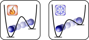
Figure 2: Two snapshots of the operation cycle of a two-level quantum heat engine. A single particle is confined in a double well potential and coupled to a thermal reservoir, whose temperature oscillates between $T^{{{\rm h}}}$ (left panel) and $T^{{{\rm c}}}<T^{{{\rm h}}}$ (right panel). In a coarse-grained picture, this setup can be described as a two-level system, where the particle is localized either in the left or in the right well. Work is extracted from the system by varying a certain external control parameter, which affects both, the energetic difference between the two minima of the potential and the height of the barrier separating them. This control operation, which corresponds to the non-classical driving protocol (80), inevitably allows the particle to tunnel between the two wells. Consequently, it will typically be found in a coherent super-position of the unperturbed energy-eigenstates during the thermodynamic cycle.

As an illustrative example for our general theory, we consider the setup sketched in Fig. 2. A two-level system with free Hamiltonian

$$H^{0}=\frac{\hbar\omega}{2}\sigma_{z}$$ (76)

is embedded in a thermal environment, which is taken into account via the unperturbed dissipation super-operator

$$\mathsf{D}^{0}\bullet\equiv\frac{\Gamma}{2}\left([\sigma_{-}\bullet,\sigma_{+}]+[\sigma_{-},\bullet\sigma_{+}]\right)\\ +\frac{\Gamma e^{-2\kappa}}{2}\left([\sigma_{+}\bullet,\sigma_{-}]+[\sigma_{+},\bullet\sigma_{-}]\right)$$ (77)

with the dimensionless parameter

$$\kappa\equiv\hbar\omega/(2k_{{{\rm B}}}T^{{{\rm c}}})$$ (78)

corresponding to the rescaled level splitting. This system is driven by the temperature profile

$$T(t)\equiv\frac{T^{{{\rm h}}}T^{{{\rm c}}}}{T^{{{\rm h}}}+(T^{{{\rm c}}}-T^{{{\rm h}}})\gamma_{q}(t)}.$$ (79)

Simultaneously, work can be extracted through the energy modulation

$$\Delta Hg_{w}(t)\equiv\Delta H\gamma_{w}(t)\left(\cos\theta\;\sigma_{z}+\sin\theta\;\sigma_{x}\right),$$ (80)

where $\gamma_{w}(t)$ and $\gamma_{q}(t)$ are $\mathcal{T}$-periodic functions of time. Furthermore, $\sigma_{x},\sigma_{y},\sigma_{z}$ denote the usual Pauli matrices and $\sigma_{\pm}\equiv(\sigma_{x}\pm i\sigma_{y})/2$. The parameter $0\leq\theta\leq\pi$ quantifies the relative degree, to which the external controller induces shifting of the free energy levels and coherent mixing between them.

The kinetic coefficients describing the thermodynamics of this system in the linear response regime can be obtained from the relation (39). To this end, we first evaluate the deviations from equilibrium

$$\delta g_{w}(t) =\gamma_{w}(t)\left(\cos\theta\;\sigma_{z}+\tanh\kappa\cos\theta\;\mathbbm{1}+\sin\theta\;\sigma_{x}\right),$$

$$\delta g_{q}(t) =-k_{{{\rm B}}}T^{{{\rm c}}}\kappa\gamma_{q}(t)\left(\sigma_{z}+\tanh\kappa\;\mathbbm{1}\right)$$ (81)

according to the definition (40). Inserting these expressions into (39), after some straightforward algebra, yields

$$L^{{{\rm cl}}}_{ab} =-\frac{\xi^{{{\rm cl}}}_{a}\xi^{{{\rm cl}}}_{b}}{k_{{{\rm B}}}\mathcal{T}}\int_{0}^{\mathcal{T}}\!\!\!dt\;\Bigl{(}\dot{\gamma}_{a}(t)\gamma_{b}(t)$$

$$\hskip 93.89418pt-\int_{0}^{\infty}\!\!\!d\tau\;\dot{\gamma}_{a}(t)\dot{\gamma}_{b}(t-\tau)e^{-\hat{\Gamma}\tau}\Bigr{)},$$

$$L_{ww}^{{{\rm qu}}} =\frac{(\xi_{w}^{{{\rm qu}}})^{2}}{k_{{{\rm B}}}\mathcal{T}}\int_{0}^{\mathcal{T}}\!\!\!dt\int_{0}^{\infty}\!\!\!d\tau\;\dot{\gamma}_{w}(t)\dot{\gamma}_{w}(t-\tau)e^{-\hat{\Gamma}\tau/2}\cos[\omega\tau],$$ (82)

where $a,b=w,q$ and the abbreviations

$$\xi_{w}^{{{\rm cl}}} \equiv\cos\theta/\cosh\kappa, \xi_{w}^{{{\rm qu}}} \equiv 2\sqrt{\kappa\tanh\kappa}\sin\theta,$$

$$\xi_{q}^{{{\rm cl}}} \equiv-k_{{{\rm B}}}T^{{{\rm c}}}\kappa/\cosh\kappa, \hat{\Gamma} \equiv\Gamma(1+e^{-2\kappa})$$ (83)

were introduced for convenience. We note that, obviously, these coefficients fulfill the symmetry relation (47) due to the driving protocol (80) satisfying the factorization condition (46). Finally, for later purposes, we evaluate the instantaneous coefficient

$$L^{{{\rm ins}}}_{qq}=\frac{(\xi_{q}^{{{\rm cl}}})^{2}\hat{\Gamma}}{k_{{{\rm B}}}\mathcal{T}}\int_{0}^{\mathcal{T}}\!\!\!dt\;\gamma_{q}^{2}(t),$$ (84)

which is defined in (35) and enters the constraint (74).

VI.2 Power and Efficiency

We will now explore the performance of the toy model of Fig. 2 as a quantum heat engine. In order to keep our analysis as simple and transparent as possible, we assume harmonic protocols

$$\gamma_{w}(t) =\sin\left[2\pi t/\mathcal{T}+\phi\right]\quad\text{and}$$

$$\gamma_{q}(t) =\left(1+\sin\left[2\pi t/\mathcal{T}\right]\right)/2,$$ (85)

where the phase shift $\phi$ can be adjusted to optimize the device for a given purpose. The kinetic coefficients (82) and (84) then become

$$L_{ww} =L_{ww}^{{{\rm cl}}}+L_{ww}^{{{\rm qu}}}=\frac{(\xi^{{{\rm cl}}}_{w})^{2}}{k_{{{\rm B}}}\mathcal{T}}\frac{\pi\alpha}{1+\alpha^{2}}$$

$$\hskip 29.4487pt+\frac{(\xi^{{{\rm qu}}}_{w})^{2}}{k_{{{\rm B}}}\mathcal{T}}\frac{2\pi\alpha\nu^{2}(4\nu^{2}+\alpha^{2}(\nu^{2}+1))}{16\nu^{4}+8\alpha^{2}\nu^{2}(\nu^{2}-4)+\alpha^{4}(\nu^{2}+4)^{2}},$$

$$L_{wq} =L_{wq}^{{{\rm cl}}}=\frac{\xi^{{{\rm cl}}}_{w}\xi^{{{\rm cl}}}_{q}}{k_{{{\rm B}}}\mathcal{T}}\frac{\pi\alpha}{1+\alpha^{2}}\frac{\cos\phi+\alpha\sin\phi}{2},$$

$$L_{qw} =L_{qw}^{{{\rm cl}}}=\frac{\xi^{{{\rm cl}}}_{w}\xi^{{{\rm cl}}}_{q}}{k_{{{\rm B}}}\mathcal{T}}\frac{\pi\alpha}{1+\alpha^{2}}\frac{\cos\phi-\alpha\sin\phi}{2},$$

$$L_{qq} =L_{qq}^{{{\rm cl}}}=\frac{(\xi^{{{\rm cl}}}_{q})^{2}}{4k_{{{\rm B}}}\mathcal{T}}\frac{\pi\alpha}{1+\alpha^{2}}$$ (86)

and

$$L_{qq}^{{{\rm ins}}}=\frac{(\xi_{q}^{{{\rm cl}}})^{2}}{k_{{{\rm B}}}\mathcal{T}}\frac{3\pi\alpha}{4},$$ (87)

respectively, with

$$\alpha\equiv\hat{\Gamma}\mathcal{T}/2\pi\quad\text{and}\quad\nu\equiv\hat{\Gamma}/\omega$$ (88)

being dimensionless constants.

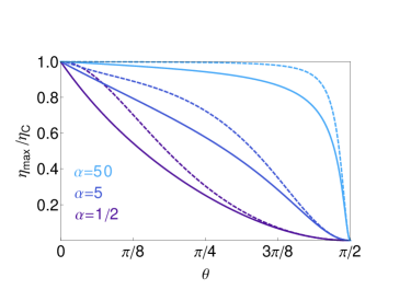
Figure 3: Maximum efficiency of a two-level quantum heat engine. The solid lines show the explicit result (89) in units of the Carnot efficiency $\eta_{{{\rm C}}}$ as function of the coherence parameter $\theta$ for different values of the damping parameter $\alpha$ . The dashed lines indicate the corresponding bound (71) evaluated with the protocols (85) and the optimal phase shift (90). The remaining parameters have been chosen as $\kappa=1/2$ and $\nu=10$. For clarity, the legend in the lower left corner follows the order of the plotted curves from top to bottom.

Within these specifications, the maximal efficiency is found by inserting (86) into (66) and (69) and taking the maximum with respect to $\phi$. This procedure yields

$$\eta_{{{\rm max}}}=\eta_{{{\rm C}}}\frac{\alpha\psi_{1}-\psi_{2}}{\alpha\psi_{1}+\psi_{2}}$$ (89)

and the corresponding optimal phase shift

$$\phi_{\eta}=\arccos[(\psi_{1}^{2}-\psi_{2}^{2})/(\psi_{1}^{2}+\psi_{2}^{2})]/2,$$ (90)

where

$$\psi_{1} \equiv\sqrt{2k_{{{\rm B}}}\mathcal{T}L^{{{\rm qu}}}_{ww}+2\pi\alpha(\xi^{{{\rm cl}}}_{w})^{2}}\quad\text{and}$$

$$\psi_{2} \equiv\alpha\sqrt{2k_{{{\rm B}}}\mathcal{T}L^{{{\rm qu}}}_{ww}}.$$ (91)

In the quasi-classical limit, where $L^{{{\rm qu}}}_{ww}$ and thus $\psi_{2}=0$, these expressions reduce to

$$\left.\eta_{{{\rm max}}}\right|_{\theta=0}=\eta_{{{\rm C}}}\quad\text{and}\quad\left.\phi_{\eta}\right|_{\theta=0}=0.$$ (92)

Hence, the engine can indeed reach Carnot efficiency if the protocols $\gamma_{w}(t)$ and $\gamma_{q}(t)$ are in phase with each other. As Fig. 3 shows, the maximum efficiency falls monotonically from $\eta_{{{\rm C}}}$ to $0$ as $\theta$ varies from $0$ to $\pi/2$. Moreover, the decay proceeds increasingly faster the smaller the damping parameter $\alpha$ is chosen. This observation can be understood intuitively, since, for large $\alpha$, the thermodynamic cycle evolves close to the adiabatic limit, where it becomes reversible. As a reference point, the bound (71) has been included in Fig. 3. It shows the same qualitative dependence on $\theta$ and $\alpha$ as the maximum efficiency, for which it provides a fairly good estimate, especially as $\theta$ comes close to $\pi/2$.

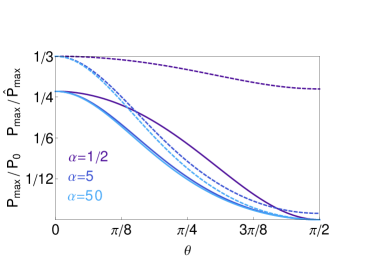
Figure 4: Dependence of the maximum power of a two-level quantum engine on the coherence parameter $\theta$ for $\kappa=1/2$, $\nu=10$ and three different values of $\alpha$. The solid lines correspond to the optimized output (93) in units of $P_{0}\equiv T^{{{\rm c}}}\mathcal{F}_{q}^{2}(\xi^{{{\rm cl}}})^{2}\alpha/(12k_{{{\rm B}}}\mathcal{T})$ Note (2). The dashed lines show the maximum power as a fraction of its upper bound (95). In the limit $\theta\rightarrow\pi/2$, both quantities, $P_{{{\rm max}}}$ and the bound $\hat{P}_{{{\rm max}}}$, vanish, while their ratio approaches a finite value. The legend in the lower left corner has been sorted according to the order of the plotted curves from top to bottom. This correspondence applies to dashed and solid lines, respectively.

We now turn to maximum power as a second important benchmark parameter. Combining (86), (66) and (72), after maximization with respect to $\phi$, yields the explicit expression

$$P_{{{\rm max}}}=\frac{T^{{{\rm c}}}\mathcal{F}_{q}^{2}}{4}\frac{\pi^{2}\alpha^{2}(\xi^{{{\rm cl}}}_{q}\xi^{{{\rm cl}}}_{w})^{2}}{2k_{{{\rm B}}}\mathcal{T}(\psi_{1}^{2}+\psi_{2}^{2})},$$ (93)

where the optimal phase shift

$$\phi_{{{\rm P}}}=\arctan\alpha$$ (94)

is independent of $\theta$. This result can be quantitatively assessed by comparing it with the bound

$$\hat{P}_{{{\rm max}}}=\frac{T^{{{\rm c}}}\mathcal{F}_{q}^{2}}{4}\frac{3\pi^{2}\alpha^{2}(\xi^{{{\rm cl}}}_{q}\xi^{{{\rm cl}}}_{w})^{2}}{2k_{{{\rm B}}}\mathcal{T}\psi_{1}^{2}},$$ (95)

which follows from (74) after inserting (87) and evaluating the parameter $z$ using the protocols (85) with $\phi=\phi_{{{\rm P}}}$.

In Fig. 4, both, the optimal power (93) and the ratio

$$\frac{P_{{{\rm max}}}}{\hat{P}_{{{\rm max}}}}=\frac{\psi_{1}^{2}}{3(\psi_{1}^{2}+\psi_{2}^{2})}$$ (96)

are plotted. Two central features of these quantities are can be observed. First $P_{{{\rm max}}}$ reaches its maximum as a function of $\theta$ in the quasi-classical case $\theta=0$ and then decays monotonically to zero as $\theta$ approaches $\pi/2$ . This behavior is in line with our general insight that coherence effects are detrimental to the performance of quantum heat engines. Second, in contrast to maximum efficiency, the maximum power comes not even close to the upper limit following from our new constraint (51). Specifically, the degree of saturation (96) is equal to $1/3$ for $\theta=0$ and then decreases even further towards $\theta=\pi/2$. Still, the bound (74) might be attainable by more complex devices than the one considered here. Whether or not such models exist remains an open question at this point.

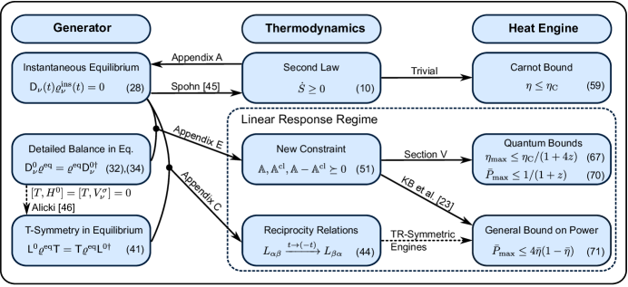
Figure 5: Flow chart visualizing the interdependence between properties of the Lindblad-generator (left column), relations between thermodynamic quantities (central column) and bounds on the performance figures of quantum heat engines (right column). Solid arrows denote unrestricted implications, while dashed arrows require the additional condition attached to them. In the last column, we used the abbreviations $\bar{\eta}\equiv\eta/\eta_{{{\rm C}}}$ and $\bar{P}_{{{\rm max}}}\equiv P_{{{\rm max}}}/P_{0}$, where $P_{0}=T^{{{\rm c}}}\mathcal{F}_{q}^{2}L_{qq}/4$ for the dashed arrow in the bottom line and otherwise $P_{0}=T^{{{\rm c}}}\mathcal{F}_{q}^{2}L_{qq}^{{{\rm ins}}}/4$. An engine is considered to be time-reversal (TR) symmetric if the corresponding driving protocols fulfill the condition (67).

VII Concluding Perspectives

In this paper, we have developed a universal framework for the description of quantum thermodynamic cycles, which allows the consistent definition of kinetic coefficients relating fluxes and affinities for small driving amplitudes. Focusing on Markovian dynamics, we have proven that these quantities fulfill generalized reciprocity relations and, moreover, are subject to a set of additional constraints. These results were derived from the characteristics of the Lindblad-generator as summarized in Fig. 5. To this end, we have invoked two fundamental physical principles. First, in order to ensure consistency with the second law, each dissipation super-operator must annihilate the instantaneous Gibbs-Boltzmann distribution at the respectively corresponding temperature. Second, we have demanded the dissipative parts of the unperturbed generator to fulfill a detailed balance relation implying zero probability flux between any pair or energy eigenstates in equilibrium. For the reciprocity relations, the even stronger $T$-symmetry condition is necessary. Both, detailed balance and $T$-symmetry are quite natural and broadly accepted conditions, which ultimately rely on the reversibility of microscopic dynamics. It should, however, be noted that, at least from a phenomenological point of view, they constitute stronger requirements than the bare second law, which stipulates only the first of the above mentioned properties of the Lindblad generator.

As a key application, our theory allows to obtain bounds on the maximum efficiency and power of quantum heat engines, which reveal that coherence effects are generally detrimental to both of these figures of merit. This insight has been illustrated quantitatively for a paradigmatic model consisting of a harmonically driven two-level system. In the quasi-classical limit, where our new constraints on the kinetic coefficients become weakest, we recover a general bound on power, which is a quadratic function of efficiency. This relation, which has been derived before for classical stochastic Brandner et al. (2015b) and thermoelectric heat engines Brandner and Seifert (2015), in particular proves the nonexistence of reversibly operating quantum devices with finite power output, at least within linear response. For classical systems, the analogous result was obtained also in Proesmans et al. (2016); Proesmans and Van den Broeck (2015) and, only recently, extended to the more general nonlinear regime in Shiraishi and Saito (2016). All of these approaches, however, rely on a Markovian dynamics, which is further specified by a detailed balance condition. Since, as we argued before, this requirement is more restrictive when demanding only the non-negativity of entropy production, the incompatibility of Carnot efficiency and finite power can not be attributed to the bare second law.

Despite the fact that our discussion has mainly focused on quantum heat engines, it is clear that our general framework covers also other types of thermal machines like, for example, quantum absorption refrigerators Levy and Kosloff (2012); Correa et al. (2014); Mitchison et al. (2015). It can be expected that the new constraints on the kinetic coefficients derived here allow to restrict also the figures of performance of such devices. Working out these bounds explicitly is left as an interesting topic for future research at this point.

Analyses of the linear response regime can provide profound insights on the properties of non-equilibrium systems. A complete understanding of their behavior, however, typically requires to take strong-driving effects into account. Quantum heat engines, for example, that are operated by purely non-classical protocols do not admit a proper linear response description, since their off-diagonal kinetic coefficients would inevitably vanish. A paradigmatic model belonging to this class is, for example, the coherently driven three-level amplifier Scovil and Schulz-DuBois (1959); Geva and Kosloff (1994, 1996). It thus emerges the question how our new constraint (51) and thus the bounds (71), (74) and (75) can be extended to the nonlinear regime. Investigations towards this direction constitute an important topic, which can be expected to be challenging, since universal results for systems arbitrary far from equilibrium are overall scarce. Indeed, the general framework of Sec. II is not tied to the assumption of small driving amplitudes. However, accounting for strong perturbations, might, for example, require to specify the dynamical generator in a more restrictive way when it was done in Sec. III thus sacrificing universality.

In summary, our approach provides an important first step towards a systematic theory of cyclic quantum thermodynamic processes. It should thus provide a fruitful basis for future investigations, which could eventually lead to a complete understanding of the fundamental principles governing the performance of quantum thermal devices.

Appendix A Thermodynamic Consistency of the Time-Dependent Lindblad Equation

We consider the total rate of entropy production (6), which can be rewritten as

$$\dot{S}[\varrho(t)] =-k_{{{\rm B}}}{{\rm tr}}\left\{\dot{\varrho}(t)\ln\varrho(t)\right\}-\sum_{\nu=1}^{N_{q}}\frac{\dot{Q}_{\nu}(t)}{T_{\nu}(t)}$$

$$=-k_{{{\rm B}}}\sum_{\nu=1}^{N_{q}}{{\rm tr}}\left\{\bigl{(}\mathsf{D}_{\nu}(t)\varrho(t)\bigr{)}\bigl{(}\ln\varrho(t)-\ln\varrho_{\nu}^{{{\rm ins}}}(t)\bigr{)}\right\}$$

$$\equiv\sum_{\nu=1}^{N_{q}}\dot{S}_{\nu}[\varrho(t)].$$ (97)

As proven by Spohn Spohn (1978), the condition (28) is sufficient for each of the contributions $S_{\nu}[\varrho(t)]$ to be non-negative for any $\varrho(t)$. Here, we show that (28) is also necessary to this end.

We proceed as follows. First, we define a one-parameter family of states $\varrho^{\lambda}_{\nu}$ such that $\varrho^{\lambda=0}_{\nu}=\varrho^{{{\rm ins}}}_{\nu}$ and $\dot{S}_{\nu}[\varrho_{\nu}^{\lambda}]$ at least once continuously-differentiable at $\lambda=0$. Hence, we obviously have

$$\left.\dot{S}_{\nu}[\varrho_{\nu}^{\lambda}]\right|_{\lambda=0}=0.$$ (98)

Note that, for convenience, we omit time-arguments from here onwards. Second, we observe that, due to continuity, the family $\varrho_{\nu}^{\lambda}$ will always contain a state $\varrho^{\lambda\ast}_{\nu}$ in the vicinity of $\lambda=0$ such that $\dot{S}_{\nu}[\varrho^{\lambda\ast}_{\nu}]<0$ unless

$$\left.\partial_{\lambda}\dot{S}_{\nu}[\varrho_{\nu}^{\lambda}]\right|_{\lambda=0}=0.$$ (99)

Third, we set

$$\varrho_{\nu}^{\lambda}=\exp[-H/(k_{{{\rm B}}}T_{\nu})+\lambda G]/Z(\lambda),$$ (100)

where $Z(\lambda)\equiv{{\rm tr}}\left\{\exp[-H/(k_{{{\rm B}}}T_{\nu})+\lambda G]\right\}$ and $G$ is an arbitrary Hermitian operator. Inserting (100) into (99) and using (97) and (24) yields

$${{\rm tr}}\left\{\bigl{(}\mathsf{D}_{\nu}\varrho^{{{\rm ins}}}_{\nu}\bigr{)}G\right\}=0.$$ (101)

Finally, this condition can only be satisfied for any Hermitian $G$ if $\mathsf{D}_{\nu}\varrho^{{{\rm ins}}}_{\nu}=0$. Thus, we have shown that, if (28) is not fulfilled, we can always construct a state $\varrho_{\nu}^{\lambda\ast}$ such that $\dot{S}_{\nu}[\varrho_{\nu}^{\lambda\ast}]$ becomes negative, which completes the proof.

Appendix B Generalized Kinetic Coefficients

B.1 General Set-up

We derive the expressions (35) for the generalized kinetic coefficients within three steps. First, by linearizing the components of the generator (22) with respect to $\Delta_{j}H$ and $\Delta_{\nu}T$, we obtain

$$\mathsf{H}(t) \equiv\mathsf{H}^{0}+\sum_{j=1}^{N_{w}}\Delta_{j}H\mathsf{H}^{wj}(t)+\mathcal{O}(\Delta^{2}),$$

$$\mathsf{D}_{\nu}(t) \equiv\mathsf{D}^{0}_{\nu}+\sum_{j=1}^{N_{w}}\Delta_{j}H\mathsf{D}^{wj}_{\nu}(t)+\Delta_{\nu}T\mathsf{D}^{q}_{\nu}(t)+\mathcal{O}(\Delta^{2}),$$ (102)

where we assume that $\mathsf{D}_{\nu}(t)$ depends on $H(t)$ and $T_{\nu}(t)$ but not on $T_{\mu}(t)$ if $\mu\neq\nu$. The quantities showing up in these expansions can be characterized as follows. A straightforward calculation shows that the structure (34) implies

$$\mathsf{D}^{0}_{\nu}\int_{0}^{1}\!\!\!d\lambda\;R^{\lambda}\bullet R^{-\lambda}\varrho^{{{\rm eq}}}=\int_{0}^{1}\!\!\!d\lambda\;R^{\lambda}\left(\mathsf{D}^{0\dagger}_{\nu}\bullet\right)R^{-\lambda}\varrho^{{{\rm eq}}},$$ (103)

where

$$\mathsf{D}^{0\dagger}_{\nu}\bullet=\frac{1}{2}\sum_{\sigma}\Gamma^{\sigma}_{\nu}\left(V_{\nu}^{\sigma}[\bullet,V^{\sigma\dagger}_{\nu}]+[V^{\sigma}_{\nu},\bullet]V^{\sigma\dagger}_{\nu}\right)\\ +\bar{\Gamma}^{\sigma}_{\nu}\left(V_{\nu}^{\sigma\dagger}[\bullet,V^{\sigma}_{\nu}]+[V^{\sigma\dagger}_{\nu},\bullet]V^{\sigma}_{\nu}\right).$$ (104)

Furthermore, by expanding the relation (28) to linear order in $\Delta_{j}H$ and $\Delta_{\nu}T$, we find

$$\mathsf{D}^{wj}_{\nu}(t)\varrho^{{{\rm eq}}} =\frac{1}{k_{{{\rm B}}}T^{{{\rm c}}}}\mathsf{D}^{0}_{\nu}\int_{0}^{1}\!\!\!d\lambda\;R^{\lambda}g_{wj}(t)R^{-\lambda}\varrho^{{{\rm eq}}},$$

$$=\frac{1}{k_{{{\rm B}}}T^{{{\rm c}}}}\int_{0}^{1}\!\!\!d\lambda\;R^{\lambda}\left(\mathsf{D}^{0\dagger}_{\nu}g_{wj}(t)\right)R^{-\lambda}\varrho^{{{\rm eq}}},$$

$$\mathsf{D}^{q}_{\nu}\varrho^{{{\rm eq}}} =\frac{1}{k_{{{\rm B}}}(T^{{{\rm c}}})^{2}}\mathsf{D}^{0}_{\nu}\int_{0}^{1}\!\!\!d\lambda\;R^{\lambda}g_{q\nu}(t)R^{-\lambda}\varrho^{{{\rm eq}}}$$

$$=\frac{1}{k_{{{\rm B}}}(T^{{{\rm c}}})^{2}}\int_{0}^{1}\!\!\!d\lambda\;R^{\lambda}\left(\mathsf{D}^{0\dagger}_{\nu}g_{q\nu}(t)\right)R^{-\lambda}\varrho^{{{\rm eq}}}.$$ (105)

Analogously, the trivial relation

$$\mathsf{H}(t)\exp[-H(t)/(k_{{{\rm B}}}T_{\nu}(t))]=0$$ (106)

yields

$$\mathsf{H}^{wj}(t)\varrho^{{{\rm eq}}} =\frac{1}{k_{{{\rm B}}}T^{{{\rm c}}}}\mathsf{H}^{0}\int_{0}^{1}\!\!\!d\lambda\;R^{\lambda}g_{wj}(t)R^{-\lambda}\varrho^{{{\rm eq}}}$$

$$=\frac{1}{k_{{{\rm B}}}T^{{{\rm c}}}}\int_{0}^{1}\!\!\!d\lambda\;R^{\lambda}\left(\mathsf{H}^{0}g_{wj}(t)\right)R^{-\lambda}\varrho^{{{\rm eq}}}.$$ (107)

As the second step of our derivation, we parametrize the density matrix $\varrho^{{{\rm c}}}(t)$ describing the limit-cycle of (21) as

$$\varrho^{{{\rm c}}}(t) \equiv\frac{1}{Z^{0}}\exp\biggl{[}-\frac{H^{0}}{k_{{{\rm B}}}T^{{{\rm c}}}}+\sum_{j=1}^{N_{w}}\frac{\Delta_{j}H}{k_{{{\rm B}}}T^{{{\rm c}}}}G_{wj}(t)$$

$$\hskip 76.82234pt+\sum_{\nu=1}^{N_{q}}\frac{\Delta_{\nu}T}{k_{{{\rm B}}}(T^{{{\rm c}}})^{2}}G_{q\nu}(t)+\mathcal{O}\left(\Delta^{2}\right)\biggr{]}$$

$$=\varrho^{{{\rm eq}}}+\sum_{j=1}^{N_{w}}\frac{\Delta_{j}H}{k_{{{\rm B}}}T^{{{\rm c}}}}\int_{0}^{1}\!\!\!d\lambda\;R^{\lambda}G_{wj}(t)R^{-\lambda}\varrho^{{{\rm eq}}}$$

$$\hskip 8.5359pt+\sum_{\nu=1}^{N_{q}}\frac{\Delta_{\nu}T}{k_{{{\rm B}}}(T^{{{\rm c}}})^{2}}\int_{0}^{1}\!\!\!d\lambda\;R^{\lambda}G_{q\nu}(t)R^{-\lambda}\varrho^{{{\rm eq}}}+\mathcal{O}\left(\Delta^{2}\right).$$ (108)

Inserting this expansion, (22) and (102) into (21) and applying the relation (103) yields

$$\partial_{t}G_{wj}(t) =\tilde{\mathsf{L}}^{0\dagger}G_{wj}(t)+\tilde{\mathsf{L}}^{0\dagger}g_{wj}(t),$$

$$\partial_{t}G_{q\nu}(t) =\tilde{\mathsf{L}}^{0\dagger}G_{q\nu}(t)+\mathsf{D}^{0\dagger}_{\nu}g_{q\nu}(t).$$ (109)

By solving these differential equations with respect to the periodic boundary conditions $G_{wj}(t+\mathcal{T})=G_{wj}(t)$ and $G_{q\nu}(t+\mathcal{T})=G_{q\nu}(t)$, we obtain

$$G_{wj}(t) =\int_{0}^{\infty}\!\!\!d\tau\;e^{\tilde{\mathsf{L}}^{0\dagger}\tau}\tilde{\mathsf{L}}^{0\dagger}g_{wj}(t-\tau),$$

$$G_{q\nu}(t) =\int_{0}^{\infty}\!\!\!d\tau\;e^{\tilde{\mathsf{L}}^{0\dagger}\tau}\mathsf{D}^{0\dagger}_{\nu}g_{q\nu}(t-\tau).$$ (110)

The integrals with infinite upper bound showing up in these expressions converge, since, due to the set of unperturbed Lindblad-operators $\{V^{\sigma}_{\nu}\}$ being self-adjoint and irreducible, the non-vanishing eigenvalues of $\tilde{\mathsf{L}}^{0\dagger}$ have negative real part Spohn (1977). Moreover, $\mathbbm{1}$ is the unique right-eigenvector of $\tilde{\mathsf{L}}^{0\dagger}$ corresponding to the eigenvalue $0$. In (110), the super-operator $e^{\tilde{\mathsf{L}}^{0\dagger}\tau}$, however, acts on operators, which, by construction, are linearly independent of $\mathbbm{1}$, since $\mathsf{D}^{0\dagger}\mathbbm{1}=0$ and $\mathsf{H}^{0}\mathbbm{1}=0$. The same argument ensures that the general expressions (35) for the kinetic coefficients are well-defined.

For the third step, we recall the definitions (30) and (31) of the generalized fluxes,

$$J_{wj} =-\frac{1}{\mathcal{T}}\int_{0}^{\mathcal{T}}\!\!\!dt\;{{\rm tr}}\left\{g_{wj}(t)\mathsf{L}(t)\varrho^{{{\rm c}}}(t)\right\}\quad\text{and}$$ (111)

$$J_{q\nu} =\frac{1}{\mathcal{T}}\int_{0}^{\mathcal{T}}\!\!\!dt\;\gamma_{q\nu}(t){{\rm tr}}\left\{H(t)\mathsf{D}^{\dagger}_{\nu}(t)\varrho^{{{\rm c}}}(t)\right\}.$$ (112)

Inserting (22), (102), (105), (107) and (108) into (111), neglecting all contributions of second order in $\Delta$ and applying (103) leads to the generalized kinetic coefficients

$$L_{wj,wk} =\frac{(-1)}{k_{{{\rm B}}}\mathcal{T}}\int_{0}^{\mathcal{T}}\!\!\!dt\;\Bigl{\langle}g_{wj}(t),\tilde{\mathsf{L}}^{0\dagger}G_{wk}(t)+\tilde{\mathsf{L}}^{0\dagger}g_{wk}(t)\Bigr{\rangle},$$

$$L_{wj,q\nu} =\frac{(-1)}{k_{{{\rm B}}}\mathcal{T}}\int_{0}^{\mathcal{T}}\!\!\!dt\;\Bigl{\langle}g_{wj}(t),\tilde{\mathsf{L}}^{0\dagger}G_{q\nu}(t)+\mathsf{D}^{0\dagger}_{\nu}g_{q\nu}(t)\Bigr{\rangle}.$$ (113)

Analogously, we obtain from (112)

$$L_{q\nu,wj} =\frac{(-1)}{k_{{{\rm B}}}\mathcal{T}}\int_{0}^{\mathcal{T}}\!\!\!dt\;\Bigl{\langle}g_{q\nu}(t),\mathsf{D}^{0\dagger}_{\nu}G_{wj}(t)+\mathsf{D}^{0\dagger}_{\nu}g_{wj}(t)\Bigr{\rangle},$$

$$L_{q\nu,q\mu} =\frac{(-1)}{k_{{{\rm B}}}\mathcal{T}}\int_{0}^{\mathcal{T}}\!\!\!dt\;\Bigl{\langle}g_{q\nu}(t),\mathsf{D}^{0\dagger}_{\nu}G_{q\mu}(t)+\delta_{\nu\mu}\mathsf{D}^{0\dagger}_{\nu}g_{q\nu}(t)\Bigr{\rangle}.$$ (114)

Finally, eliminating $G_{wj}(t)$ and $G_{q\nu}(t)$ from (113) and (114) using (110) gives the desired expressions (35).

B.2 Simplified Set-up

We consider the special case, where the system is attached only to a single reservoir. In order to derive the simplified expressions (39) for the generalized kinetic coefficients, we first note that, since $\mathsf{H}^{0}g_{q1}(t)=0$, we can replace $\mathsf{D}^{0\dagger}_{1}g_{q1}(t)$ by $\tilde{\mathsf{L}}^{0\dagger}g_{q1}(t)$ in (35). Furthermore, since also $\mathsf{H}^{0\dagger}g_{q1}(t)=0$, by virtue of (124), scalar products of the type

$$\Bigl{\langle}g_{q1}(t),\mathsf{D}_{1}^{0\dagger}\bullet\Bigr{\rangle}=\Bigl{\langle}\mathsf{D}_{1}^{0\dagger}g_{q1}(t),\bullet\Bigr{\rangle}$$ (115)

can be replaced by

$$\Bigl{\langle}\mathsf{L}^{0\dagger}g_{q1}(t),\bullet\Bigr{\rangle}=\Bigl{\langle}g_{q1}(t),\tilde{\mathsf{L}}^{0\dagger}\bullet\Bigr{\rangle}$$ (116)

such that (35) becomes

$$L_{ab}=L^{{{\rm ins}}}_{ab}+L^{{{\rm ret}}}_{ab}=-\frac{1}{k_{{{\rm B}}}\mathcal{T}}\int_{0}^{\mathcal{T}}\!\!\!dt\;\left\langle g_{a}(t),\tilde{\mathsf{L}}^{0\dagger}g_{b}(t)\right\rangle\\ -\frac{1}{k_{{{\rm B}}}\mathcal{T}}\int_{0}^{\mathcal{T}}\!\!\!dt\int_{0}^{\infty}\!\!\!d\tau\;\left\langle g_{a}(t),\tilde{\mathsf{L}}^{0\dagger}e^{\tilde{\mathsf{L}}^{0\dagger}\tau}\tilde{\mathsf{L}}^{0\dagger}g_{b}(t-\tau)\right\rangle$$ (117)

with $a,b=wj,q1$. Next, due to $\tilde{\mathsf{L}}^{0\dagger}\mathbbm{1}=\mathsf{L}^{0\dagger}\mathbbm{1}=0$, by following the same lines, we can replace $g_{a}(t)$ with $\delta g_{a}(t)$ throughout (117) thus obtaining

$$L_{ab}=-\frac{1}{k_{{{\rm B}}}\mathcal{T}}\int_{0}^{\mathcal{T}}\!\!\!dt\;\Bigl{\langle}\delta g_{a}(t),\tilde{\mathsf{L}}^{0\dagger}\delta g_{b}(t)\Bigr{\rangle}\\ -\frac{1}{k_{{{\rm B}}}\mathcal{T}}\int_{0}^{\mathcal{T}}\!\!\!dt\int_{0}^{\infty}\!\!\!d\tau\;\Bigl{\langle}\delta g_{a}(t),\tilde{\mathsf{L}}^{0\dagger}\left(\partial_{\tau}e^{\tilde{\mathsf{L}}^{0\dagger}\tau}\right)\delta g_{b}(t-\tau)\Bigr{\rangle}.$$ (118)

After one integration by parts with respect to $\tau$, this expression becomes

$$L_{ab}=\frac{(-1)}{k_{{{\rm B}}}\mathcal{T}}\int_{0}^{\mathcal{T}}\!\!\!dt\int_{0}^{\infty}\!\!\!d\tau\;\Bigl{\langle}\delta g_{a}(t),\tilde{\mathsf{L}}^{0\dagger}e^{\tilde{\mathsf{L}}^{0\dagger}\tau}\delta\dot{g}_{b}(t-\tau)\Bigr{\rangle}.$$ (119)

Here, the upper boundary term vanishes, since the super-operator $\tilde{\mathsf{L}}^{0\dagger}$ is negative semidefinite and the deviations $\delta g_{a}(t)$ are, by construction, orthogonal to its null space, which contains only scalar multiples of the unit operator.

An integration by parts with respect to $t$ transforms (119) into

$$L_{ab}=\frac{1}{k_{{{\rm B}}}\mathcal{T}}\int_{0}^{\mathcal{T}}\!\!\!dt\int_{0}^{\infty}\!\!\!d\tau\;\Bigl{\langle}\delta\dot{g}_{a}(t),\tilde{\mathsf{L}}^{0\dagger}e^{\tilde{\mathsf{L}}^{0\dagger}\tau}\delta g_{b}(t-\tau)\Bigr{\rangle},$$ (120)

where the boundary terms do not contribute due to the periodicity of the involved quantities with respect to $t$. Finally, another integration by parts with respect to $\tau$ yields (39).

Appendix C Reciprocity Relations

Our aim is to prove the reciprocity relations (44). To this end, we have to establish some technical prerequisites. First, we introduce the shorthand notation

$$L_{\alpha\beta}=-\frac{1}{k_{{{\rm B}}}\mathcal{T}}\int_{0}^{\mathcal{T}}\!\!\!dt\;\Bigl{\langle}g_{\alpha}(t),\mathsf{X}_{\alpha\beta}g_{\beta}(t)\Bigr{\rangle}\\ -\frac{1}{k_{{{\rm B}}}\mathcal{T}}\int_{0}^{\mathcal{T}}\!\!\!dt\int_{0}^{\infty}\!\!\!d\tau\;\Bigl{\langle}g_{\alpha}(t),\mathsf{Y}_{\alpha}e^{\tilde{\mathsf{L}}^{0\dagger}\tau}\mathsf{Y}_{\beta}g_{\beta}(t-\tau)\Bigr{\rangle},$$ (121)

where

$$\left(\!\begin{array}[]{cc}\mathsf{X}_{wj,wk}&\mathsf{X}_{wj,q\nu}\\ \mathsf{X}_{q\nu,wj}&\mathsf{X}_{q_{\nu},q\mu}\end{array}\!\right)\equiv\left(\!\begin{array}[]{cc}\tilde{\mathsf{L}}^{0\dagger}&\mathsf{D}^{0\dagger}\\ \mathsf{D}^{0\dagger}&\delta_{\nu\mu}\mathsf{D}^{0\dagger}\end{array}\!\right)$$ (122)

and

$$\mathsf{Y}_{wj}\equiv\tilde{\mathsf{L}}^{0\dagger},\quad\mathsf{Y}_{q\nu}\equiv\mathsf{D}^{0\dagger}.$$ (123)

Second, we note that (IV.1) and (103) imply

$$\Bigl{\langle}\bullet,\mathsf{D}^{0\dagger}\circ\Bigr{\rangle}=\Bigl{\langle}\mathsf{D}^{0\dagger}\bullet,\circ\Bigr{\rangle},\quad\Bigl{\langle}\bullet,\tilde{\mathsf{L}}^{0\dagger}\circ\Bigr{\rangle}=\Bigl{\langle}\mathsf{L}^{0\dagger}\bullet,\circ\Bigr{\rangle}.$$ (124)

Third, by virtue of (43), we have

$$\mathsf{D}^{0\dagger}=\mathsf{T}^{-1}\mathsf{D}^{0\dagger}\mathsf{T}\quad\text{and}\quad\mathsf{L}^{0\dagger}=\mathsf{T}^{-1}\tilde{\mathsf{L}}^{0\dagger}\mathsf{T},$$ (125)

where we used that the time-reversal operator is anti-unitary, i.e., $Ti+iT=0$ with $i$ denoting the imaginary unit. Combining (124), (125) with the definitions (122) and (123) yields

$$\Bigl{\langle}\bullet,\mathsf{X}_{\alpha\beta}\circ\Bigr{\rangle} =\Bigl{\langle}\mathsf{T}^{-1}\mathsf{X}_{\alpha\beta}\mathsf{T}\bullet,\circ\Bigr{\rangle}\quad\text{and}$$

$$\Bigl{\langle}\bullet,\mathsf{Y}_{\alpha}\circ\Bigr{\rangle} =\Bigl{\langle}\mathsf{T}^{-1}\mathsf{Y}_{\alpha}\mathsf{T}\bullet,\circ\Bigr{\rangle}.$$ (126)

Fourth, from the relation Mazenko (2006)

$${{\rm tr}}\left\{\bullet\right\}={{\rm tr}}\left\{\left(T\bullet T^{-1}\right)^{\dagger}\right\}$$ (127)

and the fact that $H^{0}$ commutes with $T$, it follows

$$\Bigl{\langle}\mathsf{T}^{-1}\bullet,\circ\Bigr{\rangle}=\Bigl{\langle}\bullet^{\dagger},\mathsf{T}\circ^{\dagger}\Bigr{\rangle}.$$ (128)

The reciprocity relations (44) can now be obtained through the calculation

$$L_{\alpha\beta}[g_{\alpha}(t),g_{\beta}(t)]=-\frac{1}{k_{{{\rm B}}}\mathcal{T}}\int_{0}^{\mathcal{T}}\!\!\!dt\;\Bigl{\langle}\mathsf{X}_{\alpha\beta}\mathsf{T}g_{\alpha}(t),\mathsf{T}g_{\beta}(t)\Bigr{\rangle}$$

$$\quad-\frac{1}{k_{{{\rm B}}}\mathcal{T}}\int_{0}^{\mathcal{T}}\!\!\!dt\int_{0}^{\infty}\!\!\!d\tau\;\Bigl{\langle}\mathsf{Y}_{\beta}e^{\tilde{\mathsf{L}}^{0\dagger}\tau}\mathsf{Y}_{\alpha}\mathsf{T}g_{\alpha}(t),\mathsf{T}g_{\beta}(t-\tau)\Bigr{\rangle}$$

$$=-\frac{1}{k_{{{\rm B}}}\mathcal{T}}\int_{0}^{\mathcal{T}}\!\!\!dt\;\Bigl{\langle}\mathsf{T}g_{\beta}(-t),\mathsf{X}_{\beta\alpha}\mathsf{T}g_{\alpha}(-t)\Bigr{\rangle}$$

$$\quad-\frac{1}{k_{{{\rm B}}}\mathcal{T}}\int_{0}^{\mathcal{T}}\!\!\!dt\int_{0}^{\infty}\!\!\!d\tau\;\Bigl{\langle}\mathsf{T}g_{\beta}(-t),\mathsf{Y}_{\beta}e^{\tilde{\mathsf{L}}^{0\dagger}\tau}\mathsf{Y}_{\alpha}\mathsf{T}g_{\alpha}(\tau-t)\Bigr{\rangle}$$

$$=L_{\beta\alpha}[\mathsf{T}g_{\alpha}(-t),\mathsf{T}g_{\beta}(-t)].$$ (129)

In the first step, we consecutively applied the relations (126) and (128) and exploited the properties $\left(\mathsf{X}_{\alpha\beta}\bullet\right)^{\dagger}=\mathsf{X}_{\alpha\beta}\bullet^{\dagger}$ and $\left(\mathsf{Y}_{\alpha}\bullet\right)^{\dagger}=\mathsf{Y}_{\alpha}\bullet^{\dagger}$ of the super-operators $\mathsf{X}_{\alpha\beta}$ and $\mathsf{Y}_{\alpha}$, which can be easily found by inspection. Furthermore, we used that the operators $g_{\alpha}(t)$ and $\mathsf{T}g_{\alpha}(t)$ represent observables and thus must be Hermitian. In the second step, we invoked the identities

$$\int_{0}^{\mathcal{T}}\!\!\!dt\;f(t)h(t+\tau)=\int_{0}^{\mathcal{T}}\!\!\!dt\;f(t-\tau)h(t)\quad\text{and}$$

$$\int_{0}^{\mathcal{T}}\!\!\!dt\;f(t)=\int_{0}^{\mathcal{T}}\!\!\!dt\;f(\mathcal{T}-t)=\int_{0}^{\mathcal{T}}\!\!\!dt\;f(-t),$$ (130)

which hold for any $\mathcal{T}$-periodic functions $f(t)$ and $h(t)$. Finally, we used the symmetries $\left\langle\bullet,\circ\right\rangle=\left\langle\circ,\bullet\right\rangle$ and $\mathsf{X}_{\alpha\beta}=\mathsf{X}_{\beta\alpha}$, which are direct consequences of the definitions (IV.1) and (122), respectively.

In the special case, where

$$g_{\alpha}(t)=\gamma_{\alpha}(t)g_{\alpha}$$ (131)

with $\gamma_{wj}(t)$, $g_{wj}$ introduced in (46), $\gamma_{q\nu}(t)$ defined in (9) and $g_{q\nu}\equiv-H^{0}$, (121) becomes

$$L_{\alpha\beta}[\gamma_{\alpha}(t),\gamma_{\beta}(t)]=-\frac{1}{k_{{{\rm B}}}\mathcal{T}}\int_{0}^{\mathcal{T}}\!\!\!dt\;\gamma_{\alpha}(t)\gamma_{\beta}(t)\Bigl{\langle}g_{\alpha},\mathsf{X}_{\alpha\beta}g_{\beta}\Bigr{\rangle}$$

$$\quad-\frac{1}{k_{{{\rm B}}}\mathcal{T}}\int_{0}^{\mathcal{T}}\!\!\!dt\int_{0}^{\infty}\!\!\!d\tau\;\gamma_{\alpha}(t)\gamma_{\beta}(t-\tau)\Bigl{\langle}g_{\alpha},\mathsf{Y}_{\alpha}e^{\tilde{\mathsf{L}}^{0\dagger}\tau}\mathsf{Y}_{\beta}g_{\beta}\Bigr{\rangle}$$

$$=-\frac{1}{k_{{{\rm B}}}\mathcal{T}}\int_{0}^{\mathcal{T}}\!\!\!dt\;\gamma_{\alpha}(t)\gamma_{\beta}(t)\Bigl{\langle}g_{\beta},\mathsf{X}_{\beta\alpha}g_{\alpha}\Bigr{\rangle}$$

$$\quad-\frac{1}{k_{{{\rm B}}}\mathcal{T}}\int_{0}^{\mathcal{T}}\!\!\!dt\int_{0}^{\infty}\!\!\!d\tau\;\gamma_{\alpha}(t)\gamma_{\beta}(t-\tau)\Bigl{\langle}g_{\beta},\mathsf{Y}_{\beta}e^{\tilde{\mathsf{L}}^{0\dagger}\tau}\mathsf{Y}_{\alpha}g_{\alpha}\Bigr{\rangle}$$

$$=L_{\beta\alpha}[\gamma_{\beta}(t),\gamma_{\alpha}(t)].$$ (132)

Here, for the second identity, we rearranged the scalar products following the same steps as in (129) and invoked the condition $\mathsf{T}g_{\alpha}=g_{\alpha}$. We thus have proven the relation (47).

Appendix D Role of Quantum Coherence for the Generalized Kinetic Coefficients

D.1 Quasi-Classical Systems

Our aim is to derive explicit expressions for the quasi-classical kinetic coefficients $L_{\alpha\beta}^{{{\rm cl}}}$ introduced in Sec. IV.3. To this end, we proceed in four steps. First, the condition (48) allows us to write the perturbations $g_{\alpha}(t)$ as

$$g_{\alpha}(t)=\sum_{n=1}^{M}g_{\alpha}^{n}(t)\left|n\right\rangle\left\langle n\right|,$$ (133)

where $g_{\alpha}^{n}(t)\in\mathbb{R}$ and $\left\{\left|n\right\rangle\right\}_{n=1}^{M}$ denotes the set of unperturbed energy eigenvectors corresponding to the non-degenerate eigenvalues $E^{0}_{1}<E^{0}_{2}<\cdots<E^{0}_{M}$ of $H^{0}$. Second, the commutation relations

$$[H^{0},V_{\nu}^{\sigma}]=\varepsilon^{\sigma}_{\nu}V_{\nu}^{\sigma}\quad\text{and}\quad[H^{0},V_{\nu}^{\sigma\dagger}]=-\varepsilon^{\sigma}_{\nu}V_{\nu}^{\sigma\dagger},$$ (134)

which are part of the detailed balance structure (34), identify the unperturbed Lindblad operators $V^{\sigma}_{\nu}$ and $V^{\sigma\dagger}_{\nu}$ as ladder operators with respect to $H^{0}$. Hence, their matrix elements with respect to the states $\left|n\right\rangle$ are given by

$$\langle n|V^{\sigma}_{\nu}|m\rangle =\Pi(E^{0}_{n}-E^{0}_{m}-\varepsilon^{\sigma}_{\nu})\langle nV^{\sigma}_{\nu}|m\rangle\quad\text{and}$$

$$\langle n|V^{\sigma\dagger}_{\nu}|m\rangle =\Pi(E^{0}_{n}-E^{0}_{m}+\varepsilon^{\sigma}_{\nu})\langle n|V^{\sigma\dagger}_{\nu}|m\rangle$$ (135)

with

$$\Pi(\bullet)\equiv\begin{cases}1&\text{for}\quad\bullet=0\\ 0&\text{else}\end{cases}.$$ (136)

Third, (133), (D.1) and the detailed-balance structure (104) allow us to rewrite the expressions (110) for the first-order contributions to the periodic state $\varrho^{{{\rm c}}}(t)$ as

$$\mathbf{G}_{wj}(t) =\int_{0}^{\infty}\!\!\!d\tau\;e^{\mathbb{W}^{0t}\tau}\mathbb{W}^{0t}\mathbf{g}_{wj}(t-\tau),$$

$$\mathbf{G}_{q\nu}(t) =\int_{0}^{\infty}\!\!\!d\tau\;e^{\mathbb{W}^{0t}\tau}\mathbb{W}^{0t}_{\nu}\mathbf{g}_{g\nu}(t-\tau),$$

$$\left\langle n\right|G_{\alpha}(t)\left|m\right\rangle =0\quad\text{for}\quad n\neq m.$$ (137)

Here, we used the vector notation

$$\mathbf{g}_{\alpha}(t) \equiv(g_{\alpha}^{1}(t),\dots,g_{\alpha}^{M}(t))^{t},$$

$$\mathbf{G}_{\alpha}(t) \equiv(G_{\alpha}^{1}(t),\dots,G_{\alpha}^{M}(t))^{t}\quad\text{with}$$

$$G_{\alpha}^{n}(t) \equiv\left\langle n\right|G_{\alpha}(t)\left|n\right\rangle$$ (138)

and the abbreviation

$$\mathbb{W}^{0t}\equiv\sum_{\nu=1}^{N_{q}}\mathbb{W}^{0t}_{\nu},$$ (139)

where the elements of the matrices $\mathbb{W}^{0t}_{\nu}$ are given by

$$(\mathbb{W}^{0t}_{\nu})_{mn}\equiv\begin{cases}\sum_{\sigma}\Gamma^{\sigma}_{\nu}\Pi(E^{0}_{m}-E^{0}_{n}-\varepsilon^{\sigma}_{\nu})|\langle m|V^{\sigma}_{\nu}|n\rangle|^{2},&m>n\\ \sum_{\sigma}\bar{\Gamma}^{\sigma}_{\nu}\Pi(E^{0}_{m}-E^{0}_{n}+\varepsilon^{\sigma}_{\nu})|\langle n|V^{\sigma}_{\nu}|m\rangle|^{2},&m<n\\ -\sum_{k\neq m}(\mathbb{W}^{0t}_{\nu})_{mk},&m=n\end{cases}.$$ (140)

Furthermore the superscript $t$ indicates matrix transposition. The result (137) shows that, in first order with respect to $\Delta_{j}H$ and $\Delta_{\nu}T$, the periodic state $\varrho^{{{\rm c}}}(t)$ is indeed diagonal in the eigenstates of $H^{0}$, provided the condition (48) is fulfilled. For the forth step of our derivation, we evaluate (113) and (114) using (137) thus obtaining the quasi-classical kinetic coefficients

$$L_{wj,wk}^{{{\rm cl}}} \equiv-\frac{1}{k_{{{\rm B}}}\mathcal{T}}\int_{0}^{\mathcal{T}}\!\!\!dt\;\Bigl{\langle}\mathbf{g}_{wj}(t),\mathbb{W}^{0t}\mathbf{g}_{wk}(t)\Bigr{\rangle}_{{{\rm cl}}}-\frac{1}{k_{{{\rm B}}}\mathcal{T}}\int_{0}^{\mathcal{T}}\!\!\!dt\int_{0}^{\infty}\!\!\!d\tau\;\Bigl{\langle}\mathbf{g}_{wj}(t),\mathbb{W}^{0t}e^{\mathbb{W}^{0t}\tau}\mathbb{W}^{0t}\mathbf{g}_{wk}(t-\tau)\Bigr{\rangle}_{{{\rm cl}}},$$

$$L_{wj,q\nu}^{{{\rm cl}}} \equiv-\frac{1}{k_{{{\rm B}}}\mathcal{T}}\int_{0}^{\mathcal{T}}\!\!\!dt\;\Bigl{\langle}\mathbf{g}_{wj}(t),\mathbb{W}^{0t}_{\nu}\mathbf{g}_{q\nu}(t)\Bigr{\rangle}_{{{\rm cl}}}-\frac{1}{k_{{{\rm B}}}\mathcal{T}}\int_{0}^{\mathcal{T}}\!\!\!dt\int_{0}^{\infty}\!\!\!d\tau\;\Bigl{\langle}\mathbf{g}_{wj}(t),\mathbb{W}^{0t}e^{\mathbb{W}^{0t}\tau}\mathbb{W}^{0t}_{\nu}\mathbf{g}_{q\nu}(t-\tau)\Bigr{\rangle}_{{{\rm cl}}},$$

$$L_{q\nu,wj}^{{{\rm cl}}} \equiv-\frac{1}{k_{{{\rm B}}}\mathcal{T}}\int_{0}^{\mathcal{T}}\!\!\!dt\;\Bigl{\langle}\mathbf{g}_{q\nu}(t),\mathbb{W}^{0t}_{\nu}\mathbf{g}_{wj}(t)\Bigr{\rangle}_{{{\rm cl}}}-\frac{1}{k_{{{\rm B}}}\mathcal{T}}\int_{0}^{\mathcal{T}}\!\!\!dt\int_{0}^{\infty}\!\!\!d\tau\;\Bigl{\langle}\mathbf{g}_{q\nu}(t),\mathbb{W}^{0t}_{\nu}e^{\mathbb{W}^{0t}\tau}\mathbb{W}^{0t}\mathbf{g}_{wj}(t-\tau)\Bigr{\rangle}_{{{\rm cl}}},$$

$$L_{q\nu,q\mu}^{{{\rm cl}}} \equiv-\frac{\delta_{\nu\mu}}{k_{{{\rm B}}}\mathcal{T}}\int_{0}^{\mathcal{T}}\!\!\!dt\;\Bigl{\langle}\mathbf{g}_{q\nu}(t),\mathbb{W}^{0t}_{\nu}\mathbf{g}_{q\nu}(t)\Bigr{\rangle}_{{{\rm cl}}}-\frac{1}{k_{{{\rm B}}}\mathcal{T}}\int_{0}^{\mathcal{T}}\!\!\!dt\int_{0}^{\infty}\!\!\!d\tau\;\Bigl{\langle}\mathbf{g}_{q\nu}(t),\mathbb{W}^{0t}_{\nu}e^{\mathbb{W}^{0t}\tau}\mathbb{W}^{0t}_{\mu}\mathbf{g}_{q\mu}(t-\tau)\Bigr{\rangle}_{{{\rm cl}}},$$ (141)

where the simplified scalar product is defined for arbitrary vectors $\mathbf{A}\equiv(A_{1},\dots,A_{M})^{t}\in\mathbb{R}^{M}$ and $\mathbf{B}\equiv(B_{1},\dots,B_{M})^{t}\in\mathbb{R}^{M}$ as

$$\langle\mathbf{A},\mathbf{B}\rangle_{{{\rm cl}}}\equiv\mathbf{A}^{t}\mathbb{P}^{{{\rm eq}}}\mathbf{B}$$ (142)

with $\mathbb{P}^{{{\rm eq}}}$ denoting the diagonal matrix

$$\mathbb{P}^{{{\rm eq}}}\equiv{{{\rm diag}}}(\exp[-E_{1}/(k_{{{\rm B}}}T^{{{\rm c}}})],\\ \dots,\exp[-E_{M}/(k_{{{\rm B}}}T^{{{\rm c}}})])/Z^{0}.$$ (143)

The generalized kinetic coefficients (141) describe a discrete classical system with periodically modulated energy levels

$$E_{n}(t)=E_{n}^{0}+\Delta_{j}H\sum_{j=1}^{N_{w}}g_{wj}(t),$$ (144)

whose unperturbed dynamics is governed by the master equation

$$\partial_{t}\mathbf{p}(t)=\mathbb{W}^{0}\mathbf{p}(t).$$ (145)

Here, the vector $\mathbf{p}(t)\equiv(p_{1}(t),\dots,p_{M}(t))^{t}$ contains the probabilities $p_{n}(t)$ to find the system in the state $n$ at the time $t$ and the matrix $\mathbb{W}^{0}$ obeys the classical detailed balance relation

$$\mathbb{W}^{0}\mathbb{P}^{{{\rm eq}}}=\mathbb{P}^{{{\rm eq}}}\mathbb{W}^{0t}$$ (146)

as a consequence of (34). If $N_{q}=1$, i.e., if the system is coupled only to a single reservoir, (141) can be cast into the compact form

$$L_{ab}=-\frac{1}{k_{{{\rm B}}}\mathcal{T}}\int_{0}^{\mathcal{T}}\!\!\!dt\;\Bigl{\langle}\delta\dot{\mathbf{g}}_{a}(t),\delta\mathbf{g}_{b}(t)\Bigr{\rangle}_{{{\rm cl}}}\\ +\frac{1}{k_{{{\rm B}}}\mathcal{T}}\int_{0}^{\mathcal{T}}\!\!\!dt\int_{0}^{\infty}\!\!\!d\tau\;\Bigl{\langle}\delta\dot{\mathbf{g}}_{a}(t),e^{\mathbb{W}^{0t}\tau}\delta\dot{\mathbf{g}}_{b}(t-\tau)\Bigr{\rangle}_{{{\rm cl}}},$$ (147)

where $a,b=wj,q1$ and

$$\delta\mathbf{g}_{a}(t)\equiv\mathbf{g}_{a}(t)-\mathbf{1}\langle\mathbf{1},\mathbf{g}_{a}(t)\rangle_{{{\rm cl}}}$$ (148)

with $\mathbf{1}\equiv(1,\dots,1)^{t}$. These expressions, which here arise as a special case of our general result (35), were recently derived independently in Proesmans et al. (2016); Proesmans and Van den Broeck (2015) by considering a discrete classical system from the outset.

D.2 Quantum Corrections

The decomposition (50) can be obtained from the following argument. First, we note that the super-operator $\mathsf{H}^{0}$ is skew-Hermitian with respect to the scalar product (IV.1). Second, as a consequence of the detailed balance structure (34), the super-operators $\mathsf{D}^{0\dagger}_{\nu}$ are Hermitian with respect to (IV.1) and commute with $\mathsf{H}^{0}$. Consequently, the Liouville space of the system $\mathcal{L}$ can be partitioned into subspaces that are orthogonal with respect to (IV.1) and simultaneously invariant under the action of $\mathsf{H}^{0}$ and each $\mathsf{D}^{0\dagger}_{\nu}$. In particular, such a partitioning is given by the nullsspace of $\mathsf{H}^{0}$, i.e., the set $\mathcal{L}^{{{\rm cl}}}$ of all operators commuting with $H^{0}$, and its orthogonal complement $\mathcal{L}^{{{\rm qu}}}\equiv(\mathcal{L}^{{{\rm cl}}})^{\perp}$. Since, by construction, $g_{wj}^{{{\rm cl}}}(t)\in\mathcal{L}^{{{\rm cl}}}$ and $g_{wj}^{{{\rm qu}}}(t)\in\mathcal{L}^{{{\rm qu}}}$, (50) now follows directly from the general structure of the kinetic coefficients (35).

Appendix E New Constraint

In order to prove the constraint (51), we first show that the matrix $\mathbb{A}$ defined in is positive semidefinite. To this end, we introduce the quadratic form

$$\mathcal{Q}(\mathbf{x},\mathbf{y},\mathbf{z})\equiv\mathbf{x}^{t}\mathbb{L}^{{{\rm ins}}}_{qq}\mathbf{x}+2\mathbf{x}^{t}\mathbb{L}_{qw}\mathbf{y}+2\mathbf{x}^{t}\mathbb{L}_{qq}\mathbf{z}\\ +\mathbf{y}^{t}\mathbb{L}_{ww}\mathbf{y}+\mathbf{y}^{t}\mathbb{L}_{wq}\mathbf{z}+\mathbf{z}^{t}\mathbb{L}_{qw}\mathbf{y}+\mathbf{z}^{t}\mathbb{L}_{qq}\mathbf{z},$$ (149)

where $\mathbf{x}\equiv\left(x_{1},\dots,x_{N_{q}}\right)^{t},\mathbf{z}\equiv\left(z_{1},\dots,z_{N_{q}}\right)^{t}\in\mathbb{R}^{N_{q}}$ and $\mathbf{y}\equiv\left(y_{1},\dots,y_{N_{w}}\right)^{t}\in\mathbb{R}^{N_{w}}$. We will now, one by one, cast the terms showing up on the right-hand side of (149) into a particularly instructive form. To this end, it is convenient to introduce the extended scalar product

$$\left\llangle A,B\right\rrangle\equiv\frac{1}{\mathcal{T}}\int_{0}^{\mathcal{T}}\!\!\!dt\;\left\langle A(t),B(t)\right\rangle,$$ (150)

for arbitrary time-dependent operators $A(t)$ and $B(t)$

The first term in (149) becomes

$$\mathbf{x}^{t}\mathbb{L}_{qq}^{{{\rm ins}}}\mathbf{x}=\frac{(-1)}{k_{{{\rm B}}}}\sum_{\nu=1}^{N_{q}}x_{\nu}^{2}\Bigl{\llangle}g_{q\nu},\mathsf{D}^{0\dagger}_{\nu}g_{q\nu}\Bigr{\rrangle}.$$ (151)

after inserting the definition (35) for the coefficients $L^{{{\rm ins}}}_{q\nu,q\mu}$. Using the expressions (114), the second and the third one can be respectively written as

$$2\mathbf{x}^{t}\mathbb{L}_{qw}\mathbf{y}=\frac{(-2)}{k_{{{\rm B}}}}\sum_{\nu=1}^{N_{q}}x_{\nu}\Bigl{\llangle}g_{q\nu},\mathsf{D}^{0\dagger}_{\nu}\left(G^{y}_{w}+g^{y}_{w}\right)\Bigr{\rrangle}$$ (152)

and

$$2\mathbf{x}^{t}\mathbb{L}_{qq}\mathbf{z}=\frac{(-2)}{k_{{{\rm B}}}}\sum_{\nu=1}^{N_{q}}x_{\nu}\Bigl{\llangle}g_{q\nu},\mathsf{D}^{0\dagger}_{\nu}\left(G^{z}_{q}+z_{\nu}g_{q\nu}\right)\Bigr{\rrangle}$$ (153)

with

$$g^{y}_{w}(t)\equiv\sum_{j=1}^{N_{w}}y_{j}g_{wj}(t),\quad G^{y}_{w}(t)\equiv\sum_{j=1}^{N_{w}}y_{j}G_{wj}(t)$$ (154)

and

$$G^{z}_{q}(t)\equiv\sum_{\nu=1}^{N_{q}}z_{\nu}G_{q\nu}(t).$$ (155)

We now consider the fourth term in (149). By virtue of (113), it becomes

$$\mathbf{y}^{t}\mathsf{L}_{ww}\mathbf{y}=\frac{(-1)}{k_{{{\rm B}}}}\biggl{\{}\Bigl{\llangle}g^{y}_{w}+G^{y}_{w},\tilde{\mathsf{L}}^{0\dagger}\left(G^{y}_{w}+g^{y}_{w}\right)\Bigr{\rrangle}$$

$$\hskip 113.81102pt-\Bigl{\llangle}G^{y}_{w},\tilde{\mathsf{L}}^{0\dagger}\left(G^{y}_{w}+g^{y}_{w}\right)\Bigr{\rrangle}\biggr{\}}$$

$$=\frac{(-1)}{k_{{{\rm B}}}}\biggl{\{}\Bigl{\llangle}g^{y}_{w}+G^{y}_{w},\tilde{\mathsf{L}}^{0\dagger}\left(G^{y}_{w}+g^{y}_{w}\right)\Bigr{\rrangle}-\Bigl{\llangle}G^{y}_{w},\dot{G}^{y}_{w}\Bigr{\rrangle}\biggr{\}}$$

$$=\frac{(-1)}{k_{{{\rm B}}}}\sum_{\nu=1}^{N_{q}}\Bigl{\llangle}g_{w}^{y}+G^{y}_{w},\mathsf{D}^{0\dagger}_{\nu}\left(G^{y}_{w}+g_{w}^{y}\right)\Bigr{\rrangle}.$$ (156)

For the second identity, we used the differential equation

$$\partial_{t}G^{y}_{w}(t)=\tilde{\mathsf{L}}^{0\dagger}\left(G^{y}_{w}(t)+g^{y}_{w}(t)\right),$$ (157)

which derives from (109). Since a simple integration by parts with respect to $t$ shows

$$\left\llangle A,\dot{B}\right\rrangle=-\left\llangle\dot{A},B\right\rrangle$$ (158)

for arbitrary operatros $A(t)$ and $B(t)$, the contribution $\left\llangle G_{w}^{y},\dot{G}_{w}^{y}\right\rrangle=-\left\llangle G_{w}^{y},\dot{G}_{w}^{y}\right\rrangle$ vanishes. The third identity in (156) then follows by inserting the definition (37) of $\tilde{\mathsf{L}}^{0\dagger}$ and noting that $\left\llangle\bullet,\mathsf{H}^{0}\bullet\right\rrangle=0$ due to

$$\left\llangle\bullet,\mathsf{H}^{0}\circ\right\rrangle=-\left\llangle\mathsf{H}^{0}\bullet,\circ\right\rrangle=-\left\llangle\circ,\mathsf{H}^{0}\bullet\right\rrangle.$$ (159)

The contributions $\mathbf{y}^{t}\mathbb{L}_{wq}\mathbf{z}$ and $\mathbf{z}^{t}\mathbb{L}_{qw}\mathbf{y}$ are most conveniently analyzed together. We find

$$\mathbf{y}^{t}\mathbb{L}_{wq}\mathbf{z}+\mathbf{z}^{t}\mathbb{L}_{qw}\mathbf{y} =\frac{(-1)}{k_{{{\rm B}}}}\biggl{\{}\Bigl{\llangle}G^{y}_{w}+g^{y}_{w},\tilde{\mathsf{L}}^{0\dagger}G_{q}^{z}+\sum_{\nu=1}^{N_{q}}z_{\nu}\mathsf{D}^{0\dagger}_{\nu}g_{q\nu}\Bigr{\rrangle}-\Bigl{\llangle}G^{y}_{w},\tilde{\mathsf{L}}^{0\dagger}G^{z}_{q}+\sum_{\nu=1}^{N_{q}}z_{\nu}\mathsf{D}^{0\dagger}_{\nu}g_{q\nu}\Bigr{\rrangle}$$

$$\hskip 85.35826pt+\sum_{\nu=1}^{N_{q}}\Bigl{\llangle}G^{z}_{q}+z_{\nu}g_{q\nu},\mathsf{D}^{0\dagger}_{\nu}\left(G^{y}_{w}+g_{w}^{y}\right)\Bigr{\rrangle}-\sum_{\nu=1}^{N_{q}}\Bigl{\llangle}G^{z}_{q},\mathsf{D}^{0\dagger}_{\nu}\left(G^{y}_{w}+g^{y}_{w}\right)\Bigr{\rrangle}\biggr{\}}$$

$$=\frac{(-1)}{k_{{{\rm B}}}}\biggl{\{}\sum_{\nu=1}^{N_{q}}\Bigl{\llangle}G^{y}_{w}+g^{y}_{w},\mathsf{D}^{0\dagger}_{\nu}\left(G_{q}^{z}+z_{\nu}g_{q\nu}\right)\Bigr{\rrangle}+\Bigl{\llangle}G^{y}_{w}+g^{y}_{w},\mathsf{H}^{0}G^{z}_{q}\Bigr{\rrangle}-\Bigl{\llangle}G^{y}_{w},\dot{G}^{z}_{q}\Bigr{\rrangle}$$

$$\hskip 85.35826pt+\sum_{\nu=1}^{N_{q}}\Bigl{\llangle}G^{z}_{q}+z_{\nu}g_{q\nu},\mathsf{D}^{0\dagger}_{\nu}\left(G^{y}_{w}+g_{w}^{y}\right)\Bigr{\rrangle}-\Bigl{\llangle}G^{z}_{q},\dot{G}^{y}_{w}\Bigr{\rrangle}+\Bigl{\llangle}G^{z}_{q},\mathsf{H}^{0}\left(G^{y}_{w}+g^{y}_{w}\right)\Bigr{\rrangle}\biggr{\}}$$

$$=\frac{(-1)}{k_{{{\rm B}}}}\sum_{\nu=1}^{N_{q}}\biggl{\{}\Bigl{\llangle}G^{y}_{w}+g^{y}_{w},\mathsf{D}^{0\dagger}_{\nu}\left(G_{q}^{z}+z_{\nu}g_{q\nu}\right)\Bigr{\rrangle}+\Bigl{\llangle}G^{z}_{q}+z_{\nu}g_{q\nu},\mathsf{D}^{0\dagger}_{\nu}\left(G^{y}_{w}+g_{w}^{y}\right)\Bigr{\rrangle}\biggr{\}},$$ (160)

where, for the second identity, we inserted the definition (37) of $\tilde{\mathsf{L}}^{0\dagger}$ and the differential equations (157) and

$$\partial_{t}G^{z}_{q}(t)=\tilde{\mathsf{L}}^{0\dagger}G^{z}_{q}(t)+\sum_{\nu=1}^{N_{q}}z_{\nu}\mathsf{D}^{0\dagger}_{\nu}g_{q\nu}(t)$$ (161)

following from (109). The third identity in (160) is obtained by applying (158) and (159). Finally, the last term in (149) assumes the form

$$\mathbf{z}^{t}\mathbb{L}_{qq}\mathbf{z}=\frac{(-1)}{k_{{{\rm B}}}}\sum_{\nu=1}^{N_{q}}\biggl{\{}\Bigl{\llangle}G_{q}^{z}+z_{\nu}g_{q\nu},\mathsf{D}^{0\dagger}_{\nu}\left(G_{q}^{z}+z_{\nu}g_{q\nu}\right)\Bigr{\rrangle}$$

$$\hskip 113.81102pt-\Bigl{\llangle}G_{q}^{z},\mathsf{D}^{0\dagger}_{\nu}\left(G_{q}^{z}+z_{\nu}g_{q\nu}\right)\Bigr{\rrangle}\biggr{\}}$$

$$=\frac{(-1)}{k_{{{\rm B}}}}\biggl{\{}\biggl{(}\sum_{\nu=1}^{N_{q}}\Bigl{\llangle}G_{q}^{z}+z_{\nu}g_{q\nu},\mathsf{D}^{0\dagger}_{\nu}\left(G_{q}^{z}+z_{\nu}g_{q\nu}\right)\Bigr{\rrangle}\biggr{)}$$

$$\hskip 113.81102pt-\Bigl{\llangle}G^{z}_{q},\dot{G}^{z}_{q}\Bigr{\rrangle}+\Bigl{\llangle}G^{z}_{q},\mathsf{H}^{0}G^{z}_{q}\Bigr{\rrangle}\biggr{\}}$$

$$=\frac{(-1)}{k_{{{\rm B}}}}\sum_{\nu=1}^{N_{q}}\Bigl{\llangle}G_{q}^{z}+z_{\nu}g_{q\nu},\mathsf{D}^{0\dagger}_{\nu}\left(G_{q}^{z}+z_{\nu}g_{q\nu}\right)\Bigr{\rrangle},$$ (162)

where the second identity follows from (37) and (161) and the third one from (158) and (159).

Plugging the expressions (151), (152), (153), (156), (160), (162) into (149) and recalling (124) yields

$$\mathcal{Q}(\mathbf{x},\mathbf{y},\mathbf{z})=-\frac{1}{k_{{{\rm B}}}}\sum_{\nu=1}^{N_{q}}\Bigl{\llangle}F_{\nu},\mathsf{D}^{0\dagger}_{\nu}F_{\nu}\Bigr{\rrangle}$$ (163)

with

$$F_{\nu}(t)\equiv G_{w}^{y}(t)+g_{w}^{y}(t)+G_{q}^{z}(t)+(z_{\nu}+x_{\nu})g_{q\nu}(t).$$ (164)

Since, as a consequence of the detailed balance condition (32), the super-operators $\mathsf{D}^{0\dagger}_{\nu}$ have only real, non-positive eigenvalues Spohn (1977); Frigerio (1977); Alicki and Lendi (2007), it follows $\mathcal{Q}(\mathbf{x},\mathbf{y},\mathbf{z})\geq 0$ for any $\mathbf{x},\mathbf{y},\mathbf{z}$. Moreover, the quadratic form (149) can be written as

$$\mathcal{Q}(\mathbf{x},\mathbf{y},\mathbf{z})=\mathbf{q}^{t}\mathbb{A}\mathbf{q}$$ (165)

with $\mathbf{q}\equiv\left(\mathbf{x}^{t},\mathbf{y}^{t},\mathbf{z}^{t}\right)^{t}$ and the matrix $\mathbb{A}$ defined in (56). We can thus conclude that the matrix $\mathbb{A}$ must be positive semidefinite. The second and the third relation in (51) now follow from the additive structure (50) of the kinetic coefficients by setting either $g_{wj}^{{{\rm qu}}}(t)=0$ or $g_{wj}^{{{\rm cl}}}(t)=0$.

Appendix F Quantum Refrigerators

F.1 Implementation

In this appendix, we provide a discussion of quantum refrigerators using the setup and notation of Sec. V. To this end, we assume that the thermal gradient $\mathcal{F}_{q}$ is created by two distinct reservoirs with respectively constant temperatures $T^{{{\rm c}}}$ and $T^{{{\rm h}}}>T^{{{\rm c}}}$. The flux $J_{q}$ then corresponds to the average heat withdrawal from the hot reservoir in one operation cycle. Consequently, a proper refrigerator is obtained for

$$J_{q}^{{{\rm c}}}=P-J_{q}\geq 0.$$ (166)

Here, $J_{q}^{{{\rm c}}}$ denotes the heat flux extracted from the cold reservoir and $-P=T^{{{\rm c}}}\mathcal{F}_{w}J_{w}>0$ the power supplied by the external controller. A common measure for the efficiency of such a device is the coefficient of performance Callen (1985)

$$\varepsilon\equiv-J_{q}^{{{\rm c}}}/P\leq\varepsilon_{{{\rm C}}}\equiv T^{{{\rm c}}}/(T^{{{\rm h}}}-T^{{{\rm c}}}),$$ (167)

where the upper bound $\varepsilon_{{{\rm C}}}$, which corresponds to Carnot efficiency, follows directly from the second law.

F.2 Bounds on Efficiency

Under linear response conditions, the cooling flux (166) becomes

$$J_{q}^{{{\rm c}}}=-(L_{qw}\mathcal{F}_{w}+L_{qq}\mathcal{F}_{q}),$$ (168)

since the power $P$ is of second order in the affinities. Together with the expression (65) for the work flux $J_{w}$, this relation leads to the maximum coefficient of performance

$$\varepsilon_{{{\rm max}}}=\varepsilon_{{{\rm C}}}\frac{1}{x}\frac{\sqrt{1+y}-1}{\sqrt{1+y}+1}$$ (169)

with respect to $\mathcal{F}_{w}$ Benenti et al. (2011).

In order to show how this figure is restricted by the constraint (51), it is instructive to redefine the parameter $z$ as

$$z^{{{\rm c}}}\equiv L^{{{\rm qu}}}_{ww}L_{qq}/L_{qw}^{2}\geq 0.$$ (170)

Relation (59), which follows from (51), can then be rewritten as

$$h_{z}^{{{\rm c}}}\leq y\leq 0\;\;\text{for}\;\;x<0\quad\text{and}\quad 0\leq y\leq h_{z}^{{{\rm c}}}\;\;\text{for}\;\;x\geq 0$$ (171)

with $h^{{{\rm c}}}_{z}\equiv 4x/((x-1)^{2}+4z^{{{\rm c}}})$. Consequently, we obtain the bound

$$\varepsilon_{{{\rm max}}}\leq\varepsilon_{{{\rm C}}}\frac{1}{x}\frac{\sqrt{1+h_{z}^{{{\rm c}}}}-1}{\sqrt{1+h_{z}^{{{\rm c}}}}-1}\leq\frac{\varepsilon_{{{\rm C}}}}{1+4z^{{{\rm c}}}}$$ (172)

with the second inequality being saturated only for $x\rightarrow 0$. This result proves that cyclic quantum refrigerators, at least in the linear response regime, can reach Carnot efficiency only in the quasi-classical limit, where $L_{ww}^{{{\rm qu}}}=0$ and thus $z^{{{\rm c}}}=0$. It thus completes our overall picture that coherence effects reduce the efficiency of thermal devices.

We note that the bare current (168) can not be optimized, since it is a unbounded as a function of both affinities. Bounding the cooling flux of a refrigerator generally is possible only in the nonlinear regime, which is beyond the scope of this analysis and will be left to future investigations.

References

• Callen (1985) H. B. Callen, Thermodynamics and an Introduction to Thermostatics, 2nd ed. (John Wiley & Sons, New York, 1985).
• Blickle and Bechinger (2011) V. Blickle and C. Bechinger, “Realization of a micrometer-sized stochastic heat engine,” Nat. Phys. 8, 143 (2011).
• Martínez et al. (2015) I. A. Martínez, É. Roldán, L. Dinis, D. Petrov,  and R. A. Rica, “Adiabatic Processes Realized with a Trapped Brownian Particle,” Phys. Rev. Lett. 114, 120601 (2015).
• Steeneken et al. (2010) P. G. Steeneken, K. Le Phan, M. J. Goossens, G. E. J. Koops, G. J. A. M. Brom, C. Van der Avoort,  and J. T. M. Van Beek, “Piezoresistive heat engine and refrigerator,” Nat. Phys. 7, 354 (2010).
• Koski et al. (2014) J. V. Koski, V. F. Maisi, J. P. Pekola,  and D. V. Averin, “Experimental realization of a Szilard engine with a single electron,” Proc. Natl. Acad. Sci. USA 111, 13786 (2014).
• Pekola (2015) J. P. Pekola, “Towards quantum thermodynamics in electronic circuits,” Nat. Phys. 11, 118 (2015).
• Abah et al. (2012) O. Abah, J. Roßnagel, G. Jacob, S. Deffner, F. Schmidt-Kaler, K. Singer,  and E. Lutz, “Single-ion heat engine at maximum power,” Phys. Rev. Lett. 109, 203006 (2012).
• Roßnagel et al. (2015) J. Roßnagel, S. T. Dawkins, K. N. Tolazzi, O. Abah, E. Lutz, F. Schmidt-Kaler,  and K. Singer, “A single-atom heat engine,”   (2015)arXiv:1510.03681 .
• Gardas and Deffner (2015) B. Gardas and S. Deffner, “Thermodynamic universality of quantum Carnot engines,” Phys. Rev. E 92, 042126 (2015).
• Scully (2010) M. O. Scully, “Quantum photocell: Using quantum coherence to reduce radiative recombination and increase efficiency,” Phys. Rev. Lett. 104, 207701 (2010).
• Scully et al. (2011) M. O. Scully, K. R. Chapin, K. E. Dorfman, M. B. Kim,  and A. Svidzinsky, “Quantum heat engine power can be increased by noise-induced coherence,” Proc. Amer. Math. Soc. 108, 15097 (2011).
• Horowitz and Jacobs (2014) J. M. Horowitz and K. Jacobs, “Quantum effects improve the energy efficiency of feedback control,” Phys. Rev. E 89, 042134 (2014).
• Brandner et al. (2015a) K. Brandner, M. Bauer, M. T. Schmid,  and U. Seifert, “Coherence-enhanced efficiency of feedback-driven quantum engines,” New. J. Phys. 17, 065006 (2015a).
• Mitchison et al. (2015) M. T. Mitchison, M. P. Woods, J. Prior,  and M. Huber, “Coherence-assisted single-shot cooling by quantum absorption refrigerators,” New. J. Phys. 17, 115013 (2015).
• Uzdin et al. (2015) R. Uzdin, A. Levy,  and R. Kosloff, “Equivalence of quantum heat machines, and quantum-thermodynamic signatures,” Phys. Rev. X 5, 031044 (2015).
• Hofer and Sothmann (2015) P. P. Hofer and B. Sothmann, “Quantum heat engines based on electronic Mach-Zehnder interferometers,” Phys. Rev. B 91, 195406 (2015).
• Scully et al. (2003) M. O. Scully, M. S. Zubairy, G. S. Agarwal,  and H. Walther, “Extracting work from a single heat bath via vanishing quantum coherence.” Science 299, 862 (2003).
• Dillenschneider and Lutz (2009) R. Dillenschneider and E. Lutz, “Energetics of quantum correlations,” Europhys. Lett. 88, 50003 (2009).
• Roßnagel et al. (2014) J. Roßnagel, O. Abah, F. Schmidt-Kaler, K. Singer,  and E. Lutz, “Nanoscale heat engine beyond the carnot limit,” Phys. Rev. Lett. 112, 030602 (2014).
• Abah and Lutz (2014) O. Abah and E. Lutz, “Efficiency of heat engines coupled to nonequilibrium reservoirs,” Europhys. Lett. 106, 20001 (2014).
• Manzano et al. (2015) G. Manzano, F. Galve, R. Zambrini,  and J. M. R. Parrondo, “Perfect heat to work conversion while refrigerating: thermodynamic power of the squeezed thermal reservoir,”   (2015)arXiv:1512.07881 .
• Hofer et al. (2015) P. P. Hofer, J. R. Souquet,  and A. A. Clerk, “Quantum heat engine based on photon-assisted Cooper pair tunneling,” Phys. Rev. B 93, 041418 (2016).
• Brandner et al. (2015b) K. Brandner, K. Saito,  and U. Seifert, “Thermodynamics of micro- and nano-systems driven by periodic temperature variations,” Phys. Rev. X 5, 031019 (2015b).
• Horowitz (2012) J. M. Horowitz, “Quantum-trajectory approach to the stochastic thermodynamics of a forced harmonic oscillator,” Phys. Rev. E 85, 031110 (2012).
• Horowitz and Parrondo (2013) J. M. Horowitz and J. M. R. Parrondo, “Entropy production along nonequilibrium quantum jump trajectories,” New J. Phys. 15, 085028 (2013).
• Horowitz and Sagawa (2014) J. M. Horowitz and T. Sagawa, “Equivalent definitions of the quantum nonadiabatic entropy production,” J. Stat. Phys. 156, 55 (2014).
• Jarzynski et al. (2015) C. Jarzynski, H. T. Quan,  and S. Rahav, “Quantum-classical correspondence principle for work distributions,” Phys. Rev. X 5, 031038 (2015).
• Hänggi and Talkner (2015) P. Hänggi and P. Talkner, “The other QFT,” Nat. Phys. 11, 108 (2015).
• Kohn (2001) W. Kohn, “Periodic thermodynamics,” J. Stat. Phys. 103, 417 (2001).
• Izumida and Okuda (2009) Y. Izumida and K. Okuda, “Onsager coefficients of a finite-time Carnot cycle,” Phys. Rev. E 80, 021121 (2009).
• Izumida and Okuda (2010) Y. Izumida and K. Okuda, “Onsager coefficients of a Brownian Carnot cycle,” Eur. Phys. J. B 77, 499 (2010).
• Izumida and Okuda (2015) Y. Izumida and K. Okuda, “Linear irreversible heat engines based on local equilibrium assumptions,” New. J. Phys. 17, 85011 (2015).
• Bauer et al. (2016) M. Bauer, K. Brandner,  and U. Seifert, “Optimal performance of periodically driven, stochastic heat engines under limited control,”   (2016)arXiv:1602.04119 .
• Proesmans et al. (2016) K. Proesmans, B. Cleuren,  and C. Van den Broeck, “Linear stochastic thermodynamics for periodically driven systems,” J. Stat. Mech. , 023202 (2016).
• Proesmans and Van den Broeck (2015) K. Proesmans and C. Van den Broeck, “Onsager coefficients in periodically driven systems,” Phys. Rev. Lett. 115, 090601 (2015).
• Alicki (1979) R. Alicki, “The quantum open system as a model of the heat engine,” J. Phys. A Math. Gen. 12, L103 (1979).
• Kosloff and Ratner (1984) R. Kosloff and M. A. Ratner, “Beyond linear response: Line shapes for coupled spins or oscillators via direct calculation of dissipated power,” J. Chem. Phys 80, 2352 (1984).
• Geva and Kosloff (1994) E. Geva and R. Kosloff, “Three-level quantum amplifier as a heat engine: A study in finite-time thermodynamics,” Phys. Rev. E 49, 3903 (1994).
• Breuer and Petruccione (2006) H.-P. Breuer and F. Petruccione, The Theory of Open Quantum Systems, 1st ed. (Clarendon Press, Oxford, 2006).
• Rivas and Huelga (2012) Á. Rivas and S. F. Huelga, Open Quantum Systems: An Itroduction, 1st ed. (SpringerBriefs in Physics, Heidelberg, 2012).
• Breuer et al. (2015) H.-P. Breuer, E.-M. Laine, J. Piilo,  and B. Vacchini, “Non-Markovian dynamics in open quantum systems,”   (2015), arXiv:1505.01385v1 .
• Kosloff (2013) R. Kosloff, “Quantum Thermodynamics: A Dynamical Viewpoint,” Entropy 15, 2100 (2013).
• Note (1) A set of operators $\mathcal{A}\equiv\{A_{k}\}$ is self-adjoint if for any $A_{k}\in\mathcal{A}$ also $A_{k}^{\dagger}\in\mathcal{A}$. The set is irreducible if the only operators commuting with all elements of $\mathcal{A}$ are scalar multiples of the identity.
• Spohn and Lebowitz (1978) H. Spohn and J. L. Lebowitz, “Irreversible thermodynamics for quantum systems weakly coupled to thermal reservoirs,” Adv. Chem. Phys. 38, 109 (1978).
• Spohn (1978) H. Spohn, “Entropy production for quantum dynamical semigroups,” J. Math. Phys. 19, 1227 (1978).
• Alicki (1976) R. Alicki, “On the detailed balance condition for non-Hamiltonian systems,” Rep. Math. Phys. 10, 249 (1976).
• Kossakowski et al. (1977) A. Kossakowski, A. Frigerio, V. Gorini,  and M. Verri, “Quantum detailed balance and KMS condition,” Commun. math. Phys. 57, 97 (1977).
• Frigerio and Gorini (1984) A. Frigerio and V. Gorini, “Markov dilations and quantum detailed balance,” Commun. math. Phys. 93, 517 (1984).
• Majewski (1984) W. A. Majewski, “The detailed balance condition in quantum statistical mechanics,” J. Math. Phys. 25, 614 (1984).
• Kosloff (1984) R. Kosloff, “A quantum mechanical open system as a model of a heat engine,” J. Chem. Phys. 80, 1625 (1984).
• Davies (1974) E. B. Davies, “Markovian master equations,” Commun. math. Phys. 39, 91 (1974).
• Carmichael and Walls (1976) H. J. Carmichael and D. F. Walls, “Detailed balance in open quantum Markoffian systems,” Z. Phys. B 23, 299 (1976).
• Davies (1978) E. B. Davies, “A model of heat conduction,” J. Stat. Phys. 18, 161 (1978).
• Davies and Spohn (1978) E. B. Davies and H. Spohn, “Open quantum systems with time-dependent Hamiltonians and their linear response,” J. Stat. Phys. 19, 511 (1978).
• Albash et al. (2012) T. Albash, S. Boixo, D. A. Lidar,  and P. Zanardi, “Quantum adiabatic Markovian master equations,” New J. Phys. 14, 123016 (2012).
• Zerbe and Hänggi (1995) C. Zerbe and P. Hänggi, “Brownian parametric quantum oscillator with dissipation,” Phys. Rev. E 52, 1533 (1995).
• Breuer and Petruccione (1997) H.-P. Breuer and F. Petruccione, “Dissipative quantum systems in strong laser fields: Stochastic wave-function method and Floquet theory,” Phys. Rev. A 55, 3101 (1997).
• Kohler et al. (1997) S. Kohler, T. Dittrich,  and P. Hänggi, “Floquet-Markov description of the parametrically driven, dissipative harmonic quantum oscillator,”  55, 300 (1997).
• Szczygielski et al. (2013) K. Szczygielski, D. Gelbwaser-Klimovsky,  and R. Alicki, “Markovian master equation and thermodynamics of a two-level system in a strong laser field,” Phys. Rev. E 87, 012120 (2013).
• Cuetara et al. (2015) G. B. Cuetara, A. Engel,  and M. Esposito, “Stochastic thermodynamics of rapidly driven systems,” New J. Phys. 17, 055002 (2015).
• Kubo et al. (1998) R. Kubo, M. Toda,  and N. Hashitsume, Statistical Physics II - Nonequilibrium Statistical Mechanics, 2nd ed. (Springer Series in Solid-State Sciences, 1998).
• Van Kampen (1957a) N. G. Van Kampen, “Derivation of the phenomenological equations from the master equation I - even variables only,” Physica 23, 707 (1957a).
• Van Kampen (1957b) N. G. Van Kampen, “Derivation of the phenomenological equations from the master equation II - even and odd variables,” Physica 23, 816 (1957b).
• Agarwal (1973) G. S. Agarwal, “Open quantum Markovian systems and the microreversibility,” Z. Phys. 258, 409–422 (1973).
• Mazenko (2006) G. F. Mazenko, Nonequilibrium Statistical Mechanics, 1st ed. (Wiley-VCH Verlag GmbH & Co KGaA, Weinheim, 2006).
• Onsager (1931a) L. Onsager, “Reciprocal relations in irreversible processes I,” Phys. Rev. 37, 405 (1931a).
• Onsager (1931b) L. Onsager, “Reciprocal relations in irreversible processes II,” Phys. Rev. 38, 2265 (1931b).
• Brandner and Seifert (2015) K. Brandner and U. Seifert, “Bound on thermoelectric power in a magnetic field within linear response,” Phys. Rev. E 91, 012121 (2015).
• Seifert (2012) U. Seifert, “Stochastic thermodynamics, fluctuation theorems and molecular machines.” Rep. Prog. Phys. 75, 126001 (2012).
• Schmiedl and Seifert (2008) T. Schmiedl and U. Seifert, “Efficiency at maximum power: An analytically solvable model for stochastic heat engines,” Europhys. Lett. 81, 20003 (2008).
• Holubec (2014) V. Holubec, “An exactly solvable model of a stochastic heat engine: optimization of power, power fluctuations and efficiency,” J. Stat. Mech. , P05022 (2014).
• Dechant et al. (2015) A. Dechant, N. Kiesel,  and E. Lutz, “All-optical nanomechanical heat engine,” Phys. Rev. Lett. 114, 183602 (2015).
• Dechant et al. (2016) A. Dechant, N. Kiesel,  and E. Lutz, “Underdamped stochastic heat engine at maximum efficiency,”  (2016)arXiv:1602.00392 .
• Benenti et al. (2011) G. Benenti, K. Saito,  and G. Casati, “Thermodynamic bounds on efficiency for systems with broken time-reversal symmetry,” Phys. Rev. Lett. 106, 230602 (2011).
• Brandner et al. (2013) K. Brandner, K. Saito,  and U. Seifert, “Strong bounds on Onsager coefficients and efficiency for three-terminal thermoelectric transport in a magnetic field,” Phys. Rev. Lett. 110, 070603 (2013).
• Balachandran et al. (2013) V. Balachandran, G. Benenti,  and G. Casati, “Efficiency of three-terminal thermoelectric transport under broken time-reversal symmetry,” Phys. Rev. B 87, 165419 (2013).
• Brandner and Seifert (2013) K. Brandner and U. Seifert, “Multi-terminal thermoelectric transport in a magnetic field: Bounds on Onsager coefficients and efficiency,” New. J. Phys. 15, 105003 (2013).
• Stark et al. (2014) J. Stark, K. Brandner, K. Saito,  and U. Seifert, “Classical Nernst engine,” Phys. Rev. Lett. 112, 140601 (2014).
• Note (2) Note that the standard power $P_{0}$ contains a factor $\alpha$ for the following reason. The bare maximum power (93\@@italiccorr) grows linearly in $\alpha$ and can, seemingly, become arbitrary large. However, through the optimization procedure leading to (72\@@italiccorr) the affinity $\mathcal{F}_{w}$ has been fixed as $\mathcal{F}_{w}=-\mathcal{F}_{q}L_{wq}/(2L_{ww})$. It is straightforward to check that, for $\alpha\gg 1$, the ratio of kinetic coefficients showing up here becomes proportional to $\alpha$ if the phase shift (94\@@italiccorr) is chosen. Thus, in order to stay within the linear response regime, $\mathcal{F}_{q}$ must be assumed inversely proportional to $\alpha$ such that the power output is effectively bounded.
• Shiraishi and Saito (2016) N. Shiraishi and K. Saito, “Incompatibility between Carnot efficiency and finite power in Markovian dynamics,”   (2016)arXiv:1602.03645 .
• Levy and Kosloff (2012) A. Levy and R. Kosloff, “Quantum absorption refrigerator,” Phys. Rev. Lett. 108, 070604 (2012).
• Correa et al. (2014) L. A. Correa, J. P. Palao, D. Alonso,  and G. Adesso, “Quantum-enhanced absorption refrigerators,” Sci. Rep. 4, 3949 (2014).
• Scovil and Schulz-DuBois (1959) H. E. D. Scovil and E. O. Schulz-DuBois, “Three level masers as heat engines,” Phys. Rev. Lett. 2, 262 (1959).
• Geva and Kosloff (1996) E. Geva and R. Kosloff, “The quantum heat engine and heat pump: An irreversible thermodynamic analysis of the three-level amplifier,” J. Chem. Phys. 104, 7681 (1996).
• Spohn (1977) H. Spohn, “An algebraic condition for the approach to equilibrium of an open N-level system,” Lett. Math. Phys. 2, 33 (1977).
• Frigerio (1977) A. Frigerio, “Quantum dynamical semigroups and approach to equilibrium,” Lett. Math. Phys. 2, 79 (1977).
• Alicki and Lendi (2007) R. Alicki and K. Lendi, Lect. Notes Phys., 1st ed., Vol. 717 (Springer, Berlin, Heidelberg, 2007).