Causally nonseparable processes admitting a causal model
Abstract
A recent framework of quantum theory with no global causal order predicts the existence of “causally nonseparable” processes. Some of these processes produce correlations incompatible with any causal order (they violate so-called “causal inequalities” analogous to Bell inequalities) while others do not (they admit a “causal model” analogous to a local model). Here we show for the first time that bipartite causally nonseparable processes with a causal model exist, and give evidence that they have no clear physical interpretation. We also provide an algorithm to generate processes of this kind and show that they have nonzero measure in the set of all processes. We demonstrate the existence of processes which stop violating causal inequalities but are still causally nonseparable when mixed with a certain amount of “white noise”. This is reminiscent of the behavior of Werner states in the context of entanglement and nonlocality. Finally, we provide numerical evidence for the existence of causally nonseparable processes which have a causal model even when extended with an entangled state shared among the parties.
I Introduction
It is well-known that quantum mechanics is at odds with naive notions of reality and locality as predicted by Bell’s celebrated theorem bell_einstein_1964 ; clauser_proposed_1969-1 . One might wonder whether peculiar quantum features could challenge other fundamental notions, like the concept of causality, as well. The process matrix formalism of Oreshkov, Costa and Brukner oreshkov_quantum_2012 was developed to explore this question—studying the most general causal structures compatible with local quantum mechanics for two parties and .
Surprisingly, the formalism predicts causal structures which are “causally nonseparable”: they correspond neither to being before nor to being before , nor to a probabilistic mixture thereof. These causal structures can produce correlations incompatible with any definite causal order, violating so-called “causal inequalities” oreshkov_quantum_2012 ; branciard_simplest_2016 .111For two parties, the operations implemented to violate causal inequalities have to be quantum oreshkov_quantum_2012 ; surprisingly, for three or more parties, classical operations are sufficient baumeler_maximal_2014 .
However, the empirical relevance of these results is still completely unclear. Do they appear in some physical situations or are they merely a mathematical artifact of the process matrix formalism?
For three and more parties, there are causally nonseparable processes whose physical realization is known—one instance is the “quantum switch” chiribella_quantum_2013 where the causal order between two parties and is controlled by a quantum system belonging to a third party . Processes of this kind, however, cannot violate causal inequalities araujo_witnessing_2015 ; oreshkov_causal_2015 : they admit a “causal model”, i.e., a causally separable process is capable of reproducing their correlations. Their causal nonseparability can only be certified through device-dependent “causal tomography” or “causal witnesses” araujo_witnessing_2015 . This is analogous to states which are entangled but cannot violate Bell inequalities, i.e., for which a “local model” exists werner_quantum_1989 .
Since the only causally nonseparable processes known to be physically implementable have a causal model, it is tempting to conjecture that the inability to violate causal inequalities without brukner_quantum_2014 or with oreshkov_causal_2015 operations extended to shared entangled states by all parties singles out the physical causal structures from unphysical ones. Ref. oreshkov_causal_2015 contains an example of a tripartite process matrix with a causal model but which does not remain causal under extensions, i.e., is not “extensibly causal”, demonstrating the difference between the two notions for more than two parties.
In this paper, we provide an example of a bipartite causally nonseparable process with a causal model. Furthermore, we give numerical evidence that bipartite nonseparable processes exist which do not violate causal inequalities, even when extended with entanglement. No physical interpretation is known for these processes.
The paper is organized as follows: Sec. II introduces the process matrix formalism and the definitions of causal nonseparability and causal inequalities. In Sec. III, we define a class of two-party causally nonseparable processes and construct a causal model for them. This shows that the sets of causally nonseparable and causal inequality violating processes are distinct also in the bipartite case. Since the causally nonseparable processes with a causal model can be interpreted as the mixture of physically implementable process with an unphysical process, this gives evidence that they are not implementable in nature.
In Sec. IV, we provide an algorithm to construct nonseparable processes with a causal model by composing a random causally separable process with a non-completely positive map on one party. Using a random sample generated by a “hit-and-run” Markov chain smith_monte_1980 ; smith_efficient_1984 , we also show that nonseparable processes with a causal model have nonzero measure in the space of all processes.
In Sec. V, we construct a family of “Werner processes”, which mimic the behavior of Werner states werner_quantum_1989 with respect to nonlocality and entanglement. The Werner processes’ causal nonseparability is more resistant to the introduction of “white noise” than its ability to violate causal inequalities. This shows that the analogy between causal nonseparability and causal inequalities on the one hand, and entanglement and Bell inequalities on the other, extends beyond what was previously known oreshkov_quantum_2012 ; brukner_bounding_2015 ; araujo_witnessing_2015 ; oreshkov_causal_2015 .
Finally, in Sec. VI, we examine the behavior of the processes with added shared entanglement between the parties. While some of the processes we constructed do violate causal inequalities when extended in this way (are not “extensibly causal”), numerical calculations indicate that the ability to violate causal inequalities disappears when adding a little white noise, at which the causal nonseparability is preserved. We conjecture that there are processes which are extensibly causal, and yet not physically implementable.
II Causal nonseparability and causal inequalities
Quantum circuits can be thought of as a formalization of causal structures with a definite causal order. They consist of wires, representing quantum systems, which connect boxes, representing quantum operations. While for quantum circuits, the order of the operations is fixed chiribella_theoretical_2009 , situations where the order of operations is not well-defined are readily represented in the process matrix formalism oreshkov_quantum_2012 , which can be thought of as a generalization of the quantum circuit formalism. We will briefly introduce the main elements of the formalism; a more detailed introduction to it can be found in Ref. araujo_witnessing_2015 .
A quantum operation maps a density matrix to a density matrix (where () denotes the space of linear operators on the Hilbert space ()). The most general operations within the quantum formalism are completely positive (CP) maps . Using the Choi-Jamiołkowski choi_completely_1975 ; jamiolkowski_linear_1972 (CJ) isomorphism, one can represent every CP map as an operator acting on the tensor product of the input and output Hilbert spaces:
| (1) |
where is the identity map and is a non-normalized maximally entangled state; denotes matrix transposition in the computational basis.
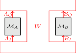
The CJ-isomorphism can also be used to represent “superoperators” or “processes” which map quantum maps to quantum maps, quantum states or probabilities gutoski_general_2007 ; chiribella_transforming_2008 ; chiribella_theoretical_2009 ; leifer_formulation_2013 ; oreshkov_quantum_2012 . In this paper, we will focus on processes mapping two quantum operations and —corresponding to the Choi-Jamiołkowski representation of Alice’s and Bob’s CP maps—to a probability (see Fig. 1). Requiring linearity of probabilities in the operations, we can represent it as
| (2) | |||
| (3) |
To ensure positivity of probabilities for all pairs of possible CP maps (as well as for extended operations where the parties share additional entanglement) the “process matrix” has to be positive semidefinite oreshkov_quantum_2012 . The normalization of probabilities implies that for all CJ-representations of completely positive trace-preserving maps and oreshkov_quantum_2012 .
We call a process () “causally ordered” if it does not allow for signalling from Bob to Alice (Alice to Bob), which is equivalent to the conditions araujo_witnessing_2015
| (4) | |||
| (5) |
A process matrix that can be decomposed into a convex combination () of causally ordered processes is “causally separable”:
| (6) |
It was recently shown that one can efficiently determine whether a process is causally (non)separable using a semidefinite program (SDP). Here we will use the SDP for “random robustness” araujo_witnessing_2015
| (7) |
where . The random robustness is defined as the result of the optimization .
If , the SDP gives an explicit decomposition of into and ; if , the process is not causally separable. The value of is also an operational measure of “causal nonseparability”. It is related to the minimal amount of “white noise” that needs to be mixed with the process to make it causally separable. That is, for , the process is causally separable.
A so-called “dual SDP” to (7) can then provide the optimal “causal witness”, i.e., a hermitian operator such that for all causally separable processes araujo_witnessing_2015 . The property can be verified experimentally by measuring a set of operators for Alice and Bob, certifying that the process is not causally separable. Note that, in analogy to entanglement witnesses chruscinski_entanglement_2014 , this certification of causal nonseparability relies on a partial tomography of the process and thus requires trust in Alice’s and Bob’s local operations: it is “device-dependent”.
It is well-known that the entanglement of a quantum state can be certified device-independently (without requiring trust Alice’s and Bob’s operations) if the probability distribution resulting from a set of measurements violates a Bell inequality acin_deviceindependent_2007 . In an analogous way, causal nonseparability can be device-independently confirmed using causal inequalities oreshkov_quantum_2012 ; branciard_simplest_2016 ; araujo_witnessing_2015 ; oreshkov_causal_2015 ; baumeler_maximal_2014 , where the “non-causal” correlations between Alice and Bob alone suffice to show that the process they use is not causally separable, without additional trust in their local operations.
The condition for a probability distribution to be “causal”, i.e., not to violate any causal inequality, is simply that it can be decomposed into a convex combination of a probability distribution which is no-signaling from Bob to Alice222When Alice is given the input and outputs (Bob is given an input and outputs ), no-signaling from Bob to Alice implies that the marginal probability on Alice’s side does not depend on Bob’s input: . () and a probability distribution which is no-signaling from Alice to Bob () branciard_simplest_2016 :
| (8) |
Note that the correlations generated by a causally ordered process cannot violate any causal inequality.
For the scenario where Alice (Bob) has an input bit () and outputs one bit (), one causal inequality is a bound on the probability of success of the “guess your neighbor’s input” (GYNI) branciard_simplest_2016 :
| (9) |
Some valid processes and local strategies which result in correlations violating (9) are described in Ref. branciard_simplest_2016 .
The relation between causally nonseparable processes and the violation of causal inequalities is not yet fully understood. On the one hand, there exist causally nonseparable processes that can be physically implemented procopio_experimental_2015 but have a causal model—they do not violate causal inequalities araujo_witnessing_2015 ; oreshkov_causal_2015 . An example of such a process is the “quantum switch” chiribella_quantum_2013 . On the other hand, there are processes that can violate causal inequalities, but it is not known if they can be realized in nature, prompting the conjecture that only processes with a causal model are physically implementable brukner_quantum_2014 .
Another natural feature to investigate is the (in)ability for a process to violate causal inequalities, even when extended with an entangled state shared by all parties. We will call processes which do not allow for such a violation “extensibly causal” oreshkov_causal_2015 and come back to this concept in detail in Sec. VI.
In the bipartite case, all previously known nonseparable processes violate causal inequalities and it is not clear if nonseparable processes with a causal model even exist branciard_simplest_2016 . In the next section, we explicitly provide a class of nonseparable bipartite processes that allow for a causal model.
III Causally nonseparable processes with a causal model
We will consider the following class of processes (all the operators are understood to act on qubits, ):
| (10) |
Here are the Pauli matrices and the tensor products between the Hilbert spaces are implicit, as in the remainder of the paper. The process matrix (10) is positive semidefinite for and causally nonseparable for . As shown in Appendix A, its random robustness is . It is maximal for , where .
The proof that the process (10) cannot be used to violate any causal inequalities, for any local strategy333Note that our proof guarantees the existence of a causal model, which means that the correlations belong to every causal polytope, without restriction on the number of inputs and outputs for each party. consists of two steps: (i) we show that the set of correlations compatible with is the same as the set of correlations achievable with (where denotes the partial transpose of the systems with respect to the computational basis); (ii) we verify that is valid and causally separable, hence cannot violate causal inequalities. Taken together, this establishes that cannot violate any causal inequalities either and therefore admits a causal model.
The first part of the proof is simple. Using definition (2) and the self-duality of transposition, we rewrite the probability distribution:
| (11) |
Additionally, for any quantum instrument davies_operational_1970 , the instrument is also valid, since transposition maps completely positive maps to completely positive maps and trace-preserving maps to trace-preserving maps444The condition on the CJ representation of a CPTP map is that and it implies .. This establishes (i), namely that the correlations achievable with are the same as those compatible with —note that this holds for any process, even when is not positive semidefinite, and therefore not a valid process matrix. In such a case, the probability distribution will be well-defined for local measurements, but not when extending the process with an entangled state between Alice and Bob, an extension which is physically meaningful and to which we will come back in Sec. VI.
For the class of process matrices given in Eq. (10), is always positive semidefinite. We will now explicitly decompose as a convex combination of causally ordered process matrices, proving that it is causally separable (formally, this implies that ).
First, one should notice the similarity of with the process matrix of a depolarizing channel (with probability of depolarizing and probability of perfectly transmitting the state) from Alice to Bob
| (12) |
where only the sign of the term differs compared to of (10). This exactly corresponds to a partial transpose of the systems , such that .
Using the definition of the depolarizing process , where . Since , we can write as:
| (13) |
which is a convex decomposition into causally ordered processes as long as . Since for the process given in Eq. (10) to be valid, and , the whole class of processes defined in Eq. (10) cannot violate causal inequalities. For a graphical representation of this relationship, see Fig. 2.
This concludes the proof and provides an explicit causal model for the process with the instruments and : the process with the instruments and . Since is causally separable, it can be interpreted as a probabilistic mixture of two causally ordered processes. There are infinitely many such decompositions since the term in Eq. (13) can be split and added to and in any proportion.
can be taken to be composed with a transpose map on . The process matrix becomes positive (meaning that the associated map is completely positive) when adding at least of white noise. However, the maximal noise that can be admixed by transferring the term in (13) is , which is strictly smaller. Therefore, the causal model for suggests a natural interpretation for it as a convex combination of an unphysical channel from Alice to Bob (as it is not completely positive) with a physical channel from Bob to Alice. This provides some evidence—yet not a proof—that the process is not physically implementable.
IV Random causally nonseparable processes with a causal model
In this section, we develop a method to construct a broad class of causally nonseparable processes with a causal model. Given a random causally separable process, one applies a positive, but not necessarily completely positive map on Bob’s side:
| (14) |
If the resulting process has negative eigenvalues, it is discarded; otherwise, it is a valid process matrix. Using the same argument as in the preceding section, we know that the resulting process will have a causal model. Sometimes—and these are the interesting cases—the process will also be causally nonseparable. This can readily be checked this via SDP (7).
We generated causally separable process matrices (where ) according to an asymptotically uniform distribution using the “hit-and-run” technique (see Appendix C for details) and Eq. (14), using the transposition map for . We found that most () of the resulting matrices were positive and hence valid process matrices. About half of these turn out to be causally nonseparable while—by construction—allowing for a causal model (we denote this set by ). The histogram of the resulting causal nonseparabilities is shown in Fig. 3.
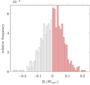
There is therefore a finite probability of generating a nonseparable process with a causal model starting from a random of causally separable process. Since the map is measure-preserving, the set of causally nonseparable processes which admit a causal model is of the same dimension as the set of valid processes itself (see Appendix B for details).
V “Werner” causally nonseparable processes
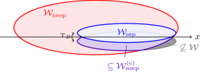
We will denote the set of causally nonseparable processes as . It is composed of the set of processes with a causal model () and the set of processes that can violate causal inequalities (), which are graphically represented in Fig. 4.
We now construct bipartite processes violating a causal inequality, but which, mixed with some amount of “white noise” , turn into causally nonseparable processes with a causal model. This behavior is reminiscent of “Werner states”, which violate Bell inequalities until a noise level of up to but are entangled when mixed with noise up to a level of werner_quantum_1989 . It shows that the analogy between causal inequalities and causal nonseparability, on the one hand, and Bell inequalities and entanglement, on the other hand, applies to the two-party case.
The idea is to use a convex combination of a process in and a process in , which is also invariant under partial transposition with respect to 555Or, in the more general scenario described in the previous section, is invariant under the non-completely-positive operation .. In this way, one can generate a broad class of “Werner causally nonseparable processes”.
We will use the process defined in Eq. (10) with the maximal causal nonseparability:
| (15) |
together with the process
| (16) |
which was proposed and shown to violate causal inequalities in Ref. oreshkov_quantum_2012 . In Appendix A, we show that the resulting mixture
| (17) |
has nonseparability , where is the random robustness of .
Following the same argument as in the previous section, we can now examine the causal nonseparability of , since, by transferring the partial transpose onto Bob’s CP maps, we know that it can produce exactly the same correlations as . Its nonseparability is again the weighted average (see Appendix A) of the nonseparabilities of and of :
| (18) |
where we used and . This means that there is a finite gap between the nonseparability of and the nonseparability of .
Using a see-saw algorithm branciard_simplest_2016 , we numerically verified that indeed violates the causal inequalities of Ref. branciard_simplest_2016 as long as is nonseparable (), i.e., when .
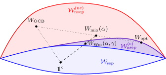
This gap translates into a gap between the level of white noise that can tolerate before admitting a causal model and the level of noise at which it becomes nonseparable. We therefore define the “Werner process” as a convex combination of and :
| (19) |
Using the definition of nonseparability (7), one can verify that the following relations hold (see Appendix A):
| (20) |
As can violate causal inequalities only if is causally nonseparable (remember the proof of Sec. III), we conclude from (20) that
| (21) |
which mimics the behavior of Werner states. See Fig. 4 for a graphical representation of the location of with respect to the different sets of processes.
VI Relationship to extensibly causal processes
In the context of the physical implementability of process matrices, it is natural to consider the extension of a process matrix with an entangled state shared between the parties. A process is “extensibly causal” if, even when extended with a shared entangled state, it cannot violate causal inequalities oreshkov_causal_2015 .
Extending a physically implementable process with an entangled state shared among the parties should also result in a physically implementable process. On this account, it is important to consider not only whether a process has a causal model, but rather whether it has such a model when extended with an entangled state. In Ref. oreshkov_causal_2015 , an example of a tripartite process with a causal model but which is not extensibly causal was presented, showing that both notions really differ and that the violation of causal inequalities can be “activated” by entanglement—and for which no physical implementation is known.
Note that the proof (Sec. III) of the existence of causal model for does not hold when the process is extended with an entangled state between Alice and Bob. It therefore cannot prove that is extensibly causal. It crucially relies on the fact that the transpose of a valid instrument for Bob is still a valid instrument. However, taking the full transpose on Bob’s instrument would lead to a “causal model” with a partial transpose of the shared entangled state, which can lead to negative probabilities. Conversely, the partial transpose of Bob’s instrument (with no transposition on Bob’s part of the entangled state) is not a valid instrument and does not yield positive probabilities in general.
To numerically study whether from Eq. (15) is extensibly causal, we extended it with a maximally entangled state of two ququarts ():
| (22) |
We chose a maximally entangled ququart state because we believe that extending with a higher dimensional state would not improve its ability to violate causal inequalities.
Using the see-saw algorithm, we optimized for a violation of the simplest causal inequalities branciard_simplest_2016 . We found that is able to violate (by about ) the GYNI inequality (9), which proves that is not extensibly causal. Incidentally, it also shows that in the bipartite case as well, the violation of causal inequalities can be “activated” using entanglement.
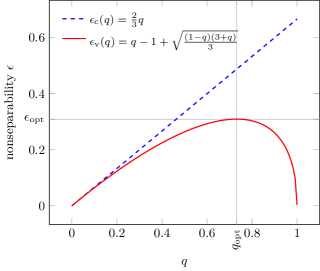
If we adopt the view that extensively causal processes are physical, the activation of violation of causal inequalities, this suffices to exclude in the same way as the tripartite process with a causal model but which is not extensibly causal, given in Ref. oreshkov_causal_2015 , independently of the argument based on the decomposition of Sec. III. However, this is not possible anymore when admixing a small amount of white noise: . We ran the see-saw algorithm for different levels of white noise and found no violation of GYNI for (see Fig. 5 for a graphical representation of the relationship between noise and violation of GYNI). Similarly, neither the other causal inequality from Ref. branciard_simplest_2016 nor the “original” causal inequality from Ref. oreshkov_quantum_2012 could be violated through see-saw optimization.
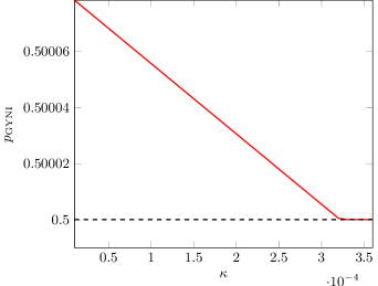
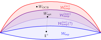
This gives reasonable evidence666It falls short of being a proof because (i) the entangled state added in is finite-dimensional; (ii) the see-saw technique is not guaranteed to converge to the global optimum; (iii) only the three known bipartite causal inequalities were tested, inequalities with more settings might still be violated. that mixed with very little white noise is extensibly causal, while still being causally nonseparable (see Fig. 6 for a graphical representation). The argument for unphysicality of Sec. III still applies to it. This leads us to conjecture that some extensibly causal processes cannot be physically realized.
VII Conclusions
We studied the classification of causally nonseparable process matrices for two parties and found that composing a class of causally separable processes with a transpose map on one party’s side results in nonseparable processes with causal models, i.e., that cannot violate causal inequalities.
Since the only interpretation we know relies on applying a non-completely positive map (which is itself is unphysical) to a valid process, the conjecture that processes which do not violate causal inequalities are physically implementable is undermined.
We also provided a simple algorithm to generate nonseparable processes with causal models—starting from a random separable process and composing it with a positive, but not completely positive map on one party’s side. With a finite probability, this yields a nonseparable process with a causal model and shows that the measure of such processes is nonzero within the space of valid processes. The “hit-and-run” algorithm we used to generate random process matrices might be of independent interest.
We then developed the analogy between entanglement/nonlocality and causal nonseparability/noncausal correlations by providing a process analogous to a Werner state: it starts having a causal model when mixed with a certain amount of white noise, while still being strictly causally nonseparable.
Finally, we studied whether our processes still have a causal model when extended with an entangled state shared between Alice and Bob (whether they are “extensibly causal”). The numerical evidence prompted us to conjecture that some of the nonseparable processes we studied are extensibly causal, while not being physically implementable.
An important question remains open: if some processes which have an (extensible) causal model are nonphysical, which other criterion should be used to rule them out? One fairly natural approach is to postulate a “purification principle”, according to which physically realizable processes can be recovered as part of a pure process in a larger space araujo_purification_???? .
Acknowledgments
We thank Ognyan Oreshkov and Fabio Costa for pointing out the significance of “extensible causal separability” in the context of physical implementability, and Ralph Silva for a useful comment on an earlier version of this manuscript. We acknowledge support from the European Commission project RAQUEL (No. 323970); the Austrian Science Fund (FWF) through the Special Research Programme FoQuS, the Doctoral Programme CoQuS and Individual Project (No. 2462) and the John Templeton Foundation.
References
- (1) J. S. Bell, “On the Einstein Podolsky Rosen paradox,” Physics 1, 195–200 (1964).
- (2) J. F. Clauser, M. A. Horne, A. Shimony, and R. A. Holt, “Proposed Experiment to Test Local Hidden-Variable Theories,” Phys. Rev. Lett. 23, 880–884 (1969).
- (3) O. Oreshkov, F. Costa, and Č. Brukner, “Quantum correlations with no causal order,” Nat. Commun. 3, 1092 (2012).
- (4) C. Branciard, M. Araújo, A. Feix, F. Costa, and Č. Brukner, “The simplest causal inequalities and their violation,” New J. Phys. 18, 013008 (2016).
- (5) Ä. Baumeler, A. Feix, and S. Wolf, “Maximal incompatibility of locally classical behavior and global causal order in multiparty scenarios,” Phys. Rev. A 90, 042106 (2014).
- (6) G. Chiribella, G. M. D’Ariano, P. Perinotti, and B. Valiron, “Quantum computations without definite causal structure,” Phys. Rev. A 88, 022318 (2013).
- (7) M. Araújo, C. Branciard, F. Costa, A. Feix, C. Giarmatzi, and Č. Brukner, “Witnessing causal nonseparability,” New J. Phys. 17, 102001 (2015).
- (8) O. Oreshkov and C. Giarmatzi, “Causal and causally separable processes,” arXiv:1506.05449.
- (9) R. F. Werner, “Quantum states with Einstein-Podolsky-Rosen correlations admitting a hidden-variable model,” Phys. Rev. A 40, 4277–4281 (1989).
- (10) Č. Brukner, “Quantum causality,” Nat. Phys. 10, 259–263 (2014).
- (11) R. L. Smith, “Monte Carlo procedures for generating random feasible solutions to mathematical programs,” in A Bulletin of the ORSA/TIMS Joint National Meeting, Washington, DC, vol. 101. 1980.
- (12) R. L. Smith, “Efficient Monte Carlo Procedures for Generating Points Uniformly Distributed over Bounded Regions,” Operations Research 32, 1296–1308 (1984).
- (13) Č. Brukner, “Bounding quantum correlations with indefinite causal order,” New J. Phys. 17, 083034 (2015).
- (14) G. Chiribella, G. M. D’Ariano, and P. Perinotti, “Theoretical framework for quantum networks,” Phys. Rev. A 80, 022339 (2009).
- (15) M.-D. Choi, “Completely positive linear maps on complex matrices,” Linear Algebra Appl. 10, 285–290 (1975).
- (16) A. Jamiołkowski, “Linear transformations which preserve trace and positive semidefiniteness of operators,” Rep. Math. Phys. 3, 275–278 (1972).
- (17) G. Gutoski and J. Watrous, “Toward a General Theory of Quantum Games,” in Proceedings of the Thirty-ninth Annual ACM Symposium on Theory of Computing, STOC ’07, pp. 565–574. ACM, New York, NY, USA, 2007.
- (18) G. Chiribella, G. M. D’Ariano, and P. Perinotti, “Transforming quantum operations: Quantum supermaps,” EPL 83, 30004 (2008).
- (19) M. S. Leifer and R. W. Spekkens, “Towards a formulation of quantum theory as a causally neutral theory of Bayesian inference,” Phys. Rev. A 88, 052130 (2013).
- (20) D. Chruściński and G. Sarbicki, “Entanglement witnesses: construction, analysis and classification,” J. Phys. A: Math. Theor. 47, 483001 (2014).
- (21) A. Acín, N. Brunner, N. Gisin, S. Massar, S. Pironio, and V. Scarani, “Device-Independent Security of Quantum Cryptography against Collective Attacks,” Phys. Rev. Lett. 98, 230501 (2007).
- (22) L. M. Procopio, A. Moqanaki, M. Araújo, F. Costa, I. Alonso Calafell, E. G. Dowd, D. R. Hamel, L. A. Rozema, Č. Brukner, and P. Walther, “Experimental superposition of orders of quantum gates,” Nat. Commun. 6, 7913 (2015).
- (23) E. B. Davies and J. T. Lewis, “An operational approach to quantum probability,” Comm. Math. Phys. 17, 239–260 (1970).
- (24) M. Araújo, A. Feix, M. Navascués, and Č. Brukner, “A purification postulate for quantum mechanics with no causal order,” (in preparation) .
- (25) L. Lovász, “Hit-and-run mixes fast,” Math. Program. 86, 443–461 (1999).
Appendix A Analytic proofs for nonseparabilities in the main text
First, we prove that the class of processes, defined by
| (23) |
has causal separability . To do so, we define a causal witness for it:
| (24) |
We first verify that is a causal witness: and , which is a sufficient condition araujo_witnessing_2015 for to have positive trace with any causally separable process. Therefore, and is indeed a causal witness.
We compute , which is negative for and implies that . From Eq. (23), it is clear that is causally separable for , so . This establishes that .
Using the same approach, we can show that the process
| (25) |
The convexity of random robustness araujo_witnessing_2015 implies that the random robustness of a convex combination is smaller than the convex combination of the random robustnesses, so . Using the same witness as before, we compute which is strictly negative when and implies that . We conclude that .
The same proof (with the same witness given in Eq. (24)) can also be used to show that the causal nonseparability of is again the convex combination .
Appendix B The dimension of the set causally separable processes
Here we show that the set of causally separable processes has the same dimension as the set of valid processes , which establishes that the set of causally separable processes has nonzero measure in the set of valid processes.
We will use the Hilbert-Schmidt decomposition of operators. An arbitrary process can be decomposed as .
The condition of normalization of probabilities, i.e., for all CJ-representations of completely positive trace-preserving maps and , implies that some terms of the Hilbert-Schmidt decomposition, corresponding to “causal loops” are excluded. In particular, for (see the Supplementary Material of Ref. oreshkov_quantum_2012 ).
Counting all the “allowed terms” in the Hilbert-Schmidt decomposition, we find that the dimension of is:
For causally ordered processes in compatible with the causal order , some additional terms, which allow for signaling from Bob to Alice, are excluded in the Hilbert-Schmidt decomposition, reducing the dimension to
This means that the set of causally ordered processes has measure zero within the set of all process matrices.
Separable processes are convex combinations of and . This means that all the terms allowed in the Hilbert-Schmidt decomposition of a valid process matrix are also allowed in the decomposition of separable processes. Therefore and share the same basis and .
Appendix C Generating uniformly distributed processes
We consider the space of process matrices as being embedded in . We wish to obtain a uniform sample of according to the -dimensional volume (Lebesgue measure), which also corresponds to the measure generated by the Hilbert-Schmidt metric. We use an adaptation of the “hit-and-run” Markov chain sampler smith_monte_1980 ; smith_efficient_1984 for this task. The iteration works as follows:
Algorithm 1
-
1.
Select a starting point .
-
2.
Choose a traceless matrix from a set of orthogonal traceless matrices and generate a random sign variable .
-
3.
Find such that is on the boundary of the set of valid processes.
-
4.
Generate a random real scalar . Take and go to step 2.
The set of directions is simply the Hilbert-Schmidt basis of allowed terms; it has dimension (see Appendix B). For bipartite processes with , there are possible directions to choose from.
Finding the intersection with the boundary of the set of positive processes in step 3 turns out to be a semidefinite program
| (26) |
However, the SDP which computes at each step of the Markov chain is a bottleneck of the algorithm. Instead, we can skip it and generate , rejecting and retrying if the resulting process is not positive:
Algorithm 2
-
1.
Select a starting point .
-
2.
Choose a traceless matrix from a set of orthogonal traceless matrices and generate a random sign variable .
-
3.
Generate a random real scalar . Take .
-
4.
If , go to step 2, otherwise repeat step 3.
The matrices are chosen to be slightly outside the set by having slightly negative eigenvalues. Therefore, there is always a finite probability of rejection at step 4, which guarantees that the algorithm samples uniformly all the way up to the boundary.
The resulting sample is uniform when two conditions hold smith_efficient_1984 . First, from every the probability to have is nonzero, which is indeed true: In steps, one can reach any starting from any . Second, the uniform distribution is a stationary distribution of the Markov chain. This is also the case: for any the probability to reach starting from in steps is the same as the probability to reach starting from in steps.
An upper bound on the convergence of the hit-and-run algorithm for convex sets (which is the case for the set ) is known—in particular, the mixing time scales as , which matches the best known mixing times for other algorithms lovasz_hitandrun_1999 . For (which is the case for ), we would need around samples to achieve the same statistical significance as from a one-dimensional hit-and-run with samples, which we deem sufficient for our purposes.
To sample uniformly distributed causally separable processes, we use the rejection method: after sampling process matrices (with a warm-up period of discarded steps), we randomly select 1000 causally separable processes (rejecting the of nonseparable ones) in the sample.
The map preserves the Lebesgue measure, since it corresponds to reflections in . Therefore, if upon applying to random causally separable matrices, there is a finite probability to obtain a valid, causally nonseparable process, this means that the set of causally nonseparable processes with a separable partial transpose is full dimensional (see Fig. 7).
