Discretized Lavrent^′ev regularization for the autoconvolution equation

Abstract.

Lavrent^′ev regularization for the autoconvolution equation was considered by J. Janno in Lavrent^′ev regularization of ill-posed problems containing nonlinear near-to-monotone operators with application to autoconvolution equation, Inverse Problems, 16(2):333–348, 2000. Here this study is extended by considering discretization of the Lavrent^′ev scheme by splines. It is shown how to maintain the known convergence rate by an appropriate choice of spline spaces and a proper choice of the discretization level. For piece-wise constant splines the discretized equation allows for an explicit solver, in contrast to using higher order splines. This is used to design a fast implementation by means of post-smoothing, which provides results, which are indistinguishable from results obtained by direct discretization using cubic splines.

Key words: autoconvolution, inverse problem, Lavrent^′ev regularization
MSC: 47J06, 47A52, 65F22

1. Introduction, problem formulation

We shall study the numerical solution of the following autoconvolution operator, say $F:L_{2}(0,1)\to L_{2}(0,1)$, given as

(1) $$[F(x)](s):=\int_{0}^{s}x(s-t)x(t)\mathrm{d}t,\quad s\in[0,1],$$

for real-valued functions. The solution to such equations attracted attention both from applications, cf. [10, 1], and from the mathematical side, see e.g. [6, 5, 3], and [2], where different approaches are taken.

Instead of the exact equation $F(x_{0})=y_{0}$ we are given noisy data $y^{\delta}$ given as

(2) $$y^{\delta}=F(x_{0})+\delta\xi$$

for given noisy right hand side. The assumption on the noise will be specified, below.

To this end we use Lavrent^′ev regularization, and hence we choose some a priori guess, say $x_{\ast}$, and a parameter $\alpha>0$ such that we look for some $x=x^{\delta}_{\alpha}$ with

(3) $$\alpha(x_{\ast}-x)+y^{\delta}=F(x).$$

Extending the analysis from [7] we want to use finite dimensional approximations to solve Eq. (2). To this end we consider linear approximations $Q=Q_{m}$ with certain approximation properties, to be specified later. Having chosen $Q_{m}$ we replace Eq. (3) by

(4) $$\alpha Q_{m}(x_{\ast}-x)+Q_{m}y^{\delta}=Q_{m}F(Q_{m}x).$$

Remark 1.

This is a two-sided discretization, since we use a finite amount of data $Q_{m}y^{\delta}$, and we also aim at representing the solution in the range of $Q_{m}$.

The outline for the material is as follows. In Section 2 we provide the error analysis for (4), extending Janno’s original ideas, where no discretization was involved. These results are then extended in Section 3. We also derive an explicit implementation of the scheme (4). Finally we provide some numerical study, where we discuss the control of the involved parameters, in particular the choice of $\alpha$, and the discretization level $m$, both as functions of the noise level $\delta$, which is assumed to be known. Most of the proofs are given in the appendix.

2. Error analysis of the discretized regularization problem

The goal is to formulate the main results. To do so we first introduce the basic assumptions, then we derive some properties of the autoconvolution operator. Special attention is paid on the approximation of the value $x_{0}(0)$, since this will prove important. The main results and some consequences are then given in § 2.4.

2.1. Assumptions

The error analysis will be based on several assumptions, especially on the noise, the (unknown) solution $x$ in (2), and the discretization schemes, to be considered.

We shall consider two different assumptions on the noise.

Assumption 1 (noise).

Suppose that we are given a noise level $\delta>0$.

1. The element $\xi$ obeys $\left\|\xi\right\|_{\infty}\leq\delta.$

2. The element $\xi$ obeys $\left\|\xi\right\|_{2}\leq\delta.$

The main result, Theorem 1 is concerned with the first case, Assumption 1(1), and we shall briefly discuss the more relaxed assumption 1(2) in its Corollary 1.

We turn to the solution smoothness. For $x\in L_{\infty}(0,1)$ we will denote the essential supremum norm of $x$ as $\|x\|_{\infty}$.

Assumption 2 (solution smoothness).

The unknown solution element $x_{0}$ is positive, it belongs to $W^{2}_{\infty}(0,1)$, and $\left\|x_{0}\right\|_{C^{1}(0,1)}\leq K$, where we equip the space $C^{1}(0,1)$ with norm $\left\|x\right\|_{C^{1}(0,1)}:=\max\left\{\left\|x\right\|_{\infty},\left\|x^{\prime}\right\|_{\infty}\right\}$. In particular we assume that $x_{0}(0)>0$.

Remark 2.

Since we assumed that the unknown solution is positive and the autoconvolution of a positive function is obviously nonnegative, we know that the exact data $y_{0}:=F(x_{0})$ are nonnegative. For this reason we will assume that our noisy data are nonnegative as well, otherwise we would define new data $\tilde{y}^{\delta}$ by

$$\tilde{y}^{\delta}(s)=\begin{cases}y^{\delta}(s)&\text{ if }y^{\delta}(s)\geq 0\\ 0&\text{ else}\end{cases}$$

without increasing the noise level.

Following the study [7], having fixed some $\sigma\geq 0$ (to be specified later) we equip $L_{2}(0,1)$ with the inner product

$$\langle x,y\rangle_{\sigma}=\int_{0}^{1}e^{-2\sigma t}x(t)y(t)\mathrm{d}t,$$

and the corresponding (weighted) norm

$$\|x\|_{\sigma}^{2}=\int_{0}^{1}e^{-2\sigma t}x(t)^{2}\mathrm{d}t.$$

Although the norms $\left\|\cdot\right\|$ and $\left\|\cdot\right\|_{\sigma}$ are equivalent, i.e., for fixed $\sigma>0$ we have that

(5) $$e^{-\sigma}\|x\|_{0}\leq\|x\|_{\sigma}\leq\|x\|_{0},\quad x\in L_{2}(0,1),$$

we shall occasionally denote the weighted Hilbert space by $L_{2}^{\sigma}(0,1)$. There is a natural isometry $D_{\sigma}\colon L_{2}(0,1)\to L_{2}^{\sigma}(0,1)$, given through the function $f_{\sigma}(t)=e^{\sigma t},\ t\in[0,1]$ as

(6) $$D_{\sigma}x=f_{\sigma}x,\quad x\in L_{2}(0,1).$$

Similarly, if $x\in L_{2}(0,1)$ is such that it is absolutely continuous, and the weak derivatives are in $L_{2}(0,1)$, then we shall denote the weighted Sobolev Hilbert space of such elements by $H^{\sigma}_{1}(0,1)$, equipped with norm

$$\left\|x\right\|_{1,\sigma}:=\frac{1}{2}\left(\left\|x\right\|_{\sigma}^{2}+\left\|x^{\prime}\right\|_{\sigma}^{2}\right)^{1/2}.$$

Furthermore we introduce the operator norm $\left\|.\right\|_{\sigma\to\sigma}$ as

$$\left\|A\right\|_{\sigma\to\sigma}:=\left\|A\colon L_{2}^{\sigma}(0,1)\to L_{2}^{\sigma}(0,1)\right\|=\sup_{x\in L_{2}^{\sigma}(0,1)}\frac{\left\|Ax\right\|_{\sigma}}{\left\|x\right\|_{\sigma}}.$$

for linear Operators $A:L_{2}^{\sigma}(0,1)\to L_{2}^{\sigma}(0,1)$.

Remark 3.

Note that $\|.\|_{\sigma}$ reduces to the standard $L_{2}$-norm for $\sigma=~{}0$. Also, due to the above equivalence, the spaces $H^{\sigma}_{1}(0,1)$ are equivalent to the usual Sobolev Hilbert spaces $H^{1}(0,1)$. Finally, we mention that functions $x\in C^{1}(0,1)$ belong to $H^{\sigma}_{1}(0,1)$ and $\left\|x\right\|_{H_{1}^{\sigma}(0,1)}\leq\left\|x\right\|_{C^{1}(0,1)}$.

We turn to describing the approximation scheme, captured by the approximation operators $Q_{m},\ m=1,2,\dots$

Assumption 3 (approximation power).

We assume that we are given a sequence $X_{m}\subset L_{2}(0,1),\ m\in\mathbb{N}$, of finite dimensional subspaces, $\dim(X_{m})=m$ with orthogonal (in $L_{2}^{\sigma}(0,1)$) projections $Q_{m}^{\sigma}$ onto the spaces $X_{m}$. There is a constant $L<\infty$ such that for all $x\in H^{\sigma}_{1}(0,1)$ we have

(7) $$\inf\left\{\left\|x-z\right\|_{\sigma},\quad z\in X_{m}\right\}\leq\frac{L}{m}\left\|x\right\|_{H^{\sigma}_{1}(0,1)},\quad m\in\mathbb{N}.$$

We highlight the relations and approximation properties between the unweighted ($\sigma=0$) and weighted ($\sigma>0$) spaces. Specifically, any family of projection operators $(Q_{m})_{m\in\mathbb{N}}$, which fulfills assumption 3 for $\sigma=0$ can be used to construct projection operators $Q_{m}^{\sigma}$ for $\sigma>0$, which also satisfy assumption 3, with simple proof to be found in the appendix.

Lemma 1.

Let $X_{m}\subset L_{2}(0,1),\ m\in\mathbb{N}$ a sequence of finite dimensional subspaces with orthogonal (in $L_{2}(0,1)$) projections $Q_{m}$ onto the spaces $X_{m}$, satisfying Assumption 3 with a constant $L<\infty$. Moreover let $f_{\sigma}$ and $D_{\sigma}$ as in (6). Then for $\sigma>0$ the projection operators $Q_{m}^{\sigma}$ defined by

(8) $$Q_{m}^{\sigma}:=D_{\sigma}Q_{m}D_{\sigma}^{{}^{-1}}$$

are orthogonal projection operators w.r.t. $\langle.,.\rangle_{\sigma}$, for which Assumption 3 holds with constant $\sqrt{2}\left(1+\sigma\right)L$, onto the spaces $D_{\sigma}X_{m}$.

We provide the following illustrative examples.

Example 1 (piece-wise constant splines).

We let $\tilde{X}_{m}$ be the spline spaces $\mathcal{S}^{m}_{1}$ of piece-wise constant functions with respect to the equi-distant partition $\Delta_{i}=[(i-1)/m,i/m),\ i=1,\dots,m$. The spaces $X_{m}$ are then given as $X_{m}=D_{\sigma}(\tilde{X}_{m})$.

The approximation power for elements in $H^{1}(0,1)$ by piece-wise constant functions is known (cf. [11, Thm. 6.1, eq. (6.7)] with p=q=2) as

(9) $$\inf\left\{\left\|x-z\right\|_{,}\quad z\in X_{m}\right\}\leq\frac{L}{m}\left\|x\right\|_{H_{1}(0,1)},\quad m\in\mathbb{N},$$

and hence the spaces $\tilde{X}_{m}$ obey Assumption 3 for $\sigma=0$ with constant $L=1$. By virtue of Lemma 1 this extends to the spaces $X_{m}$. We mention that this approximation maps nonnegative functions to nonnegative piece-wise constant functions.

Example 2 (cubic splines).

As above we consider the equidistant partition, and we let $\mathcal{S}_{4}^{m}$ be the space of cubic splines, with corresponding orthogonal (in $L_{2}(0,1)$) projection $Q_{m}$. Then Assumption 3 holds, and we refer to the comprehensive monograph [11, Cor. 6.26] (with $m=4,\sigma=1,p=q=2,r=0$) for $\sigma=0$. Therefore, the validity of Assumption 3 extends to $\sigma>0$.

Actually, for functions which fulfill Assumption 2 we even have the stronger assertion

$$\inf\left\{\left\|x-z\right\|_{\infty},\quad z\in X_{m}\right\}\leq\frac{L}{m^{2}}\left\|x\right\|_{W^{2}_{\infty}(0,1)},\quad m\in\mathbb{N},$$

see e.g. [11, Cor. 6.26] (with $m=4,\sigma=2,p=q=\infty,r=0$). However, we cannot benefit from this additional approximation power in the overall performance of the proposed Lavrent^′ev regularization.

2.2. Properties of the autoconvolution operator

In the subsequent analysis we will relate the nonlinear autoconvolution equation (1) to the following linear Volterra equation. We note that for $F$ from (1) its Frèchet-derivative $F^{\prime}(x)\colon L_{2}(0,1)\to L_{2}(0,1)$, at element $x$, is given by

(10) $$[F^{\prime}(x)h](s)=2\int_{0}^{s}x(s-t)h(t)\mathrm{d}t,\quad s\in[0,1],\ h\in L_{2}(0,1).$$

Under the assumptions made on the solution $x_{0}$ the equation

(11) $$F^{\prime}(x_{0})\omega=x_{0}-x_{0}(0),$$

has a solution, and we refer to [7, Lemma 4].

We bound the norm of the Frèchet derivative in the weighted Hilbert spaces $L_{2}^{\sigma}(0,1)$.

Lemma 2.

For the Frèchet-derivative $F^{\prime}(u)$ of $F$ at $u\in L_{2}^{\sigma}(0,1)$ the estimate

$$\|F^{\prime}(u)\colon L_{2}^{\sigma}(0,1)\to L_{2}^{\sigma}(0,1)\|\leq 2\|u\|_{\sigma},\quad u\in L_{2}^{\sigma}(0,1),$$

holds. Consequently, we also have that

(12) $$\|F(x)\|_{\sigma}\leq\|x\|_{\sigma}^{2},\quad x\in L_{2}^{\sigma}(0,1).$$

Proof.

Let $u\in L_{2}^{\sigma}(0,1)$. Then we have

$$\|F^{\prime}(u)v\|_{\sigma}^{2}= \int_{0}^{1}e^{-2\sigma s}\left(2\int_{0}^{s}u(s-t)v(t)\mathrm{d}t\right)^{2}\mathrm{d}s$$

$$= 4\int_{0}^{1}\left(\int_{0}^{s}e^{-\sigma(s-t)}u(s-t)e^{-\sigma t}v(t)\mathrm{d}t\right)^{2}\mathrm{d}s$$

$$\leq 4\int_{0}^{1}\left(\int_{0}^{s}e^{-2\sigma(s-t)}u(s-t)^{2}\mathrm{d}t\right)\left(\int_{0}^{s}e^{-2\sigma t}v(t)^{2}\mathrm{d}t\right)\mathrm{d}s$$

$$\leq 4\int_{0}^{1}\left(\int_{0}^{1}e^{-2\sigma t}u(t)^{2}\mathrm{d}t\right)\left(\int_{0}^{1}e^{-2\sigma t}v(t)^{2}\mathrm{d}t\right)\mathrm{d}s$$

$$= 4\|u\|_{\sigma}^{2}\|v\|_{\sigma}^{2}.$$

The final assertions follows from the observation that $F(x)=\frac{1}{2}F^{\prime}(x)x$, which completes the proof. ∎

The following technical lemma will be used to prove the main result.

Lemma 3 (cf. [7, Lem. 3 & 4]).

Suppose that $x_{0}$ obeys Assumption 2. For each $0<c<1$ there is some $\sigma_{0}\geq 0$ such that for $\sigma\geq\sigma_{0}$ we have that

1. $\langle F^{\prime}(x_{0})v,v\rangle_{\sigma}\geq 0,\quad v\in L_{2}(0,1)$, and

2. the solution $\omega$ to (11) obeys $\left\|\omega\right\|_{\sigma}<c$.

2.3. Approximation of the initial value

Recall, for the solution to the equation (11) to exist, we required to know the value $x_{0}(0)$. Since this is not the case, we need to find a good approximation to it, based on the given data $y^{\delta}$. This is done by averaging with the approximating mapping $Q_{m}^{0}$ from example 1, formulated in the following proposition, again with proof postponed to the Appendix.

Proposition 1.

Let $\sigma>0$, $\delta\leq 1$ and $m\in\mathbb{N}$ be fixed, with $m\geq 1/\delta$. If the noise obeys Assumption 1(1) then

$$\left|\sqrt{\frac{1}{\sqrt{\delta}}{[Q_{m}y^{\delta}](\sqrt{\delta})}}-x_{0}(0)\right|\leq\frac{\left(1+{4\left\|x_{0}\right\|_{C^{1}(0,1)}^{2}}\right)}{x_{0}(0)}\sqrt{\delta},$$

if $[Q_{m}y^{\delta}](\sqrt{\delta})\geq 0$ and

$$\left|x_{0}(0)\right|\leq\frac{\left(1+{4\left\|x_{0}\right\|_{C^{1}(0,1)}^{2}}\right)}{x_{0}(0)}\sqrt{\delta},$$

otherwise.

Thus we use the approximation as found in Proposition 1 to define the reference element $x_{\ast}$. Specifically, given $\delta>0$ we let $x_{\ast}$ be the constant function defined as

(13) $$x_{\ast}\equiv\begin{cases}\sqrt{\frac{1}{\sqrt{\delta}}{[Q_{m}y^{\delta}](\sqrt{\delta}})},&\text{ if }[Q_{m}y^{\delta}](\sqrt{\delta})\geq 0\\ 0,&\text{ else.}\end{cases}$$

The above approximation cannot be used for general noise which just belongs to $L_{2}(0,1)$. We give the following result for this case.

Proposition 2.

Suppose that the noise obeys Assumption 1(2). Then there is a constant $D<\infty$ such that for $h:=\left(\frac{2}{3}\|x_{0}\|^{2}_{C^{1}(0,1)}\right)^{-\frac{2}{5}}\delta^{\frac{2}{5}}$ we have that

$$\left|\sqrt{\frac{2}{h^{2}}\int_{0}^{h}y^{\delta}(t)\mathrm{d}t}-x_{0}(0)\right|\leq\frac{D}{x_{0}(0)}\delta^{\frac{2}{5}},\quad\text{as}\ \delta\to 0.$$

Remark 4.

Estimation of the derivative of a function under $L_{2}$-noise has not been studied as often. The best results in this direction are presented in [9, 8]. This will not immediately give results under the smoothness Assumption 2. It is not clear to the authors, whether a reconstruction rate $\delta^{1/2}$ is possible under $L_{2}$-noise.

2.4. Main result

We now recall the equation (4), as

(14) $$Q(\alpha(x_{*}-x)+y^{\delta}-F(Qx))=0,$$

where $Q$ is any, not necessarily orthogonal, projection. We are interested in its solution. Therefore we introduce the family of linear operators $H_{\alpha}:=\left(\alpha\operatorname{Id}+QF^{\prime}(x_{0})Q\right),\ \alpha>0$. For projections $Q$ onto some space $X_{m}\subset X$, orthogonal in a suited $L_{2}^{\sigma}(0,1)$ the mapping $H_{\alpha}$ is continuously invertible, and maps $X_{m}$ into $X_{m}$, which is easy to check. For given $\alpha>0$, to be specified later, we apply $H_{\alpha}^{-1}$ to both sides. We see that

$$0= H_{\alpha}^{-1}Q\big{(}\alpha(x_{*}-x)+y^{\delta}-F(Qx)\big{)}$$

$$= H_{\alpha}^{-1}Q\big{(}y^{\delta}-F(x_{0})-F^{\prime}(x_{0})(Qx-x_{0})-F(Qx-x_{0})+\alpha(x_{*}-x)\big{)}$$

$$= H_{\alpha}^{-1}\Big{(}-\big{(}QF^{\prime}(x_{0})(Q(x-x_{0}))+\alpha(Qx-x_{0})\big{)}+QF^{\prime}(x_{0})(x_{0}-Qx_{0})$$

$$\qquad\ \ +Q\big{(}y^{\delta}-y_{0}-F(Qx-x_{0})\big{)}+\alpha(Qx_{*}-x_{0})\Big{)}$$

$$= x_{0}-Qx+$$

$$\begin{split}H_{\alpha}^{-1}\Big{(}Q\big{(}F^{\prime}(x_{0})(x_{0}-Qx_{0})+y^{\delta}-y_{0}-F(Q_{m}x-x_{0})\big{)}+\alpha(Qx_{*}-x_{0})\Big{)}.\end{split}$$

This can be written as a fixed-point equation for the (continuous nonlinear) mapping $G\colon X\to X$, given by

(15) $$\begin{split}G(Qx):=x_{0}+H_{\alpha}^{-1}\Big{(}Q\big{(}F^{\prime}(x_{0})(x_{0}-Qx_{0})+y^{\delta}-y_{0}\\ -F(Q_{m}x-x_{0})\big{)}+\alpha(Qx_{*}-x_{0})\Big{)},\ x\in L_{2}^{\sigma}(0,1).\end{split}$$

The fixed-point equation we consider is now given as

(16) $$G(Qx)=Qx,$$

on some domain to be determined later. The following holds true.

Proposition 3.

Let $\sigma>0$ be such that $F^{\prime}(x_{0})$ is accretive on $L_{2}^{\sigma}(0,1)$. Suppose that $m\geq\sigma/\delta$, $\delta\leq 1$ and that the element $\omega$ as the solution to (11) satisfies $\left\|\omega\right\|_{\sigma}<1/4$. If the noise obeys Assumption 1(1) then there is some $r>0$ such that the mapping $G$ obeys

$$G\left(B(x_{0},r)\cap X_{m}\right)\subset B(x_{0},r)\cap X_{m}.$$

Consequently it has a fixed point.

We are now in the position to formulate the main result,

Theorem 1.

Suppose that the noise obeys Assumption 1(1), and that the true solution obeys Assumption 2, and that the discretization is with spaces $X_{m}$ which fulfill Assumption 3. Moreover let the assumptions of Proposition 3 hold. There is a constant $c>0$ such that for $\alpha:=c\sqrt{\delta}$, Lavrent^′ev regularization with discretization according to (4) has a solution $x^{\delta}_{\alpha}\in X_{m}$ which obeys

$$\left\|x_{0}-x^{\delta}_{\alpha}\right\|\leq c\sqrt{\delta},\quad\text{as}\ \delta\to 0.$$

Again, we postpone the proofs, both for Proposition 3 and Theorem 1 to the Appendix.

We shall next mention the modification of the main results when the noise obeys Assumption 1(2). As the interested reader may check, the arguments used in the proofs of Proposition 3 and Theorem 1 remain valid, except that the optimal parameter choice strategy is different.

Corollary 1.

Under the assumptions of Theorem 1, but with noise fulfilling Assumption 1(2) we have the following. There is a constant $c>0$ such that for the parameter $\alpha$ is chosen from

$$\alpha=c\delta^{\frac{2}{5}}$$

this yields

$$\left\|x_{0}-x^{\delta}_{\alpha}\right\|\leq c\delta^{\frac{2}{5}},\quad\text{as}\ \delta\to 0.$$

3. Extension

We will extend the main results to the situation when the projections used in (14) are not orthogonal, but the corresponding spaces $X_{m}$ still obey Assumption 3.

As we know from Lemma 3 we can choose the value of $\sigma>0$ such that accretivity of the operator $F^{\prime}(x_{0})$ holds in $L_{2}^{\sigma}(0,1)$. This, of course, extends to accretivity of the mapping $QF^{\prime}(x_{0})Q$, whenever $Q$ is an orthogonal projection in $L_{2}^{\sigma}(0,1)$.

In some cases, the accretivity extends at the expense of an additional correction term to nonorthogonal projections. The prototypical example is the projection onto the piece-wise constant functions, which is orthogonal in $L_{2}(0,1)$, but not in $L_{2}^{\sigma}(0,1)$. The following ’closeness’ can be established.

Lemma 4.

Consider the spaces $\tilde{X}_{m}$ as in Example 1, and let $Q_{m}:=Q_{m}^{0}$ be the projection, which is orthogonal in $L_{2}(0,1)$. Then, for $m\geq\sigma$ we have that

$$\left\|Q_{m}-Q_{m}^{\sigma}\right\|_{\sigma\to\sigma}\leq 2\frac{\sigma}{m}.$$

Consequently we find that

$$\left\|Q_{m}\right\|_{\sigma\to\sigma}\leq 1+2\frac{\sigma}{m}.$$

As a consequence of the preceding lemma we obtain

Corollary 2.

Suppose that $\sigma>0$ is chosen such that $Q_{m}^{\sigma}F^{\prime}(x_{0})Q_{m}^{\sigma}$ is accretive w.r.t. $\langle.,.\rangle_{\sigma}$. Then $Q_{m}F^{\prime}(x_{0})Q_{m}+\frac{8\sigma\|x_{0}\|}{m}\operatorname{Id}$ is accretive w.r.t. $\langle.,.\rangle_{\sigma}$. Consequently

$$\|(\alpha\operatorname{Id}+Q_{m}F^{\prime}(x_{0})Q_{m})^{-1}\|_{\sigma}\leq\frac{2}{\alpha}$$

and

$$\|(\alpha\operatorname{Id}+Q_{m}F^{\prime}(x_{0})Q_{m})^{-1}Q_{m}F^{\prime}(x_{0})Q_{m}\|_{\sigma}\leq 2$$

for $\alpha\geq\frac{16\sigma\|x_{0}\|}{m}$.

Based on these preliminary results, we show that in the setting of Example 1 the result of Theorem 1 can also be obtained with the projections $Q_{m}:=Q_{m}^{0}$ even for $\sigma>0$.

Proposition 4.

Let $\sigma>0$ and $Q_{m},Q_{m}^{\sigma}$ as in Lemma 4. We denote the projection space corresponding to $Q_{m}$ by $X_{m}^{0}$. For the noise level $0<\delta\leq 1$ assume that we have $m\delta\geq 1$. Then the Lavrent^′ev-regularized equation

(17) $$\alpha Q_{m}(x_{\ast}-x)+Q_{m}y^{\delta}=Q_{m}F(Q_{m}x).$$

has a solution $x^{\delta}_{\alpha}\in X_{m}^{0}$ with

$$\left\|x_{0}-x^{\delta}_{\alpha}\right\|\leq c\sqrt{\delta},$$

for a suitable parameter choice $\alpha=c\sqrt{\delta}$ with some constant $c$ (independent of $\delta$).

The proofs of the previous results, Lemma 4, Corollary 2, and Proposition 4 are given in the appendix.

4. Numerical simulation

Here we are going to highlight the validity of the theoretical findings. Also, we want to discuss that some of the theoretical limitations cannot be seen in practical simulations. This concerns the assumption of the accretivity, i.e., when we require $\sigma$ to be chosen according to Lemma 3.

4.1. An explicit solver

We shall show that the discretization described in Example 1 leads to a convenient explicit scheme for solving the discretized equation (4) with $Q_{m}:=Q_{m}^{\sigma}$. Thus, we fix $\sigma>0$, and $m\in\mathbb{N}$, and we consider the orthogonal projection $Q_{m}^{\sigma}$ from Example 1.

First we simplify the operator $Q_{m}^{\sigma}\circ F\circ Q_{m}^{\sigma}$. Therefore we define for $x\in L_{2}(0,1)$ , and for $1\leq i\leq m$, the quantities

$$f_{i}(s) :=\begin{cases}e^{\sigma s},&\text{ for }\frac{i-1}{m}\leq s\leq\frac{i}{m},\\ 0,&\text{ else},\end{cases}$$

and

$$x^{i} :=m\int_{\frac{i-1}{m}}^{\frac{i}{m}}e^{-\sigma t}x(t)\mathrm{d}t.$$

In these terms we see that

$$Q_{m}^{\sigma}x=\sum_{i=1}^{m}x^{i}f_{i},\quad x\in L_{2}(0,1).$$

We identify $\mathcal{R}(Q_{m}^{\sigma})$ with a vector in $\mathbb{R}^{m}$ through the bijection

$$x\longrightarrow(x^{i})_{1\leq i\leq m}.$$

Furthermore, let

$$h_{i}(s):=\begin{cases}\frac{i-1}{m}+s&\text{ for }\frac{i-1}{m}\leq s<\frac{i}{m}\\ \frac{i+1}{m}-s&\text{ for }\frac{i}{m}\leq s<\frac{i+1}{m}\\ 0&\text{ else}\end{cases}$$

Then for $x\in L_{2}(0,1)$ we have

$$(Q_{m}^{\sigma}\circ F\circ Q_{m}^{\sigma})(x)= (Q_{m}^{\sigma}\circ F)\left(\sum_{i=1}^{m}x^{i}f_{i}\right)$$

$$= Q_{m}^{\sigma}\left(\sum_{i=1}^{m}\sum_{j=1}^{m-i+1}x^{i}x^{j}f_{i}*f_{j}\right)$$

$$= Q_{m}^{\sigma}\left(\sum_{k=1}^{m}\sum_{j=1}^{k}x^{k-j+1}x^{j}(f_{k}+f_{k+1})h_{k}\right)$$

$$= \frac{1}{2m}\sum_{k=1}^{m}\sum_{j=1}^{k}x^{k-j+1}x^{j}(f_{k}+f_{k+1}).$$

Now we can write equation (14) component-wise as follows. For $i=1$ we find that $x^{1}$ must satisfy the quadratic equation

$$\left(x^{1}\right)^{2}+2m\alpha x^{1}-\left(2m\left(y^{\delta}\right)^{1}+2m\alpha x_{\ast}^{1}\right)=0.$$

Note that $(y^{\delta})^{i}\geq 0$ for all $i=1,\dots,n$, since we can assume that $y^{\delta}\geq 0$ (see remark 2). The non-negative solution is

(18) $$x^{1}=-m\alpha+\sqrt{m^{2}\alpha^{2}+2m((y^{\delta})^{1}+\alpha x_{*}^{1})}.$$

For $i=2,\dots,m$ we find that

(19) $$\alpha(x_{*}^{i}-x^{i})+(y^{\delta})^{i}-\frac{1}{2m}\left(\sum_{j=1}^{i}x^{i-j+1}x^{j}+\sum_{j=1}^{i-1}x^{i-j}x^{j}\right)=0.$$

This can be considered as a linear equation in $x^{i}$, if all $x_{j}$ for $j<i$ are already determined. Rearrangement yields

(20) $$x^{i}=\frac{m}{m\alpha+x^{1}}\left((y^{\delta})^{i}+\alpha x_{*}^{i}-\frac{1}{2m}\left(\sum_{j=1}^{i-1}x^{j}x^{i-j}+\sum_{j=2}^{i-1}x^{j}x^{i-j+1}\right)\right).$$

Thus we have obtained the piece-wise constant approximation $Q_{m}^{\sigma}x$, and we now apply post-smoothing by a cubic spline. By doing this appropriately we can retain approximation rate $\frac{1}{2}$. Indeed, consider a cubic spline $S\in S_{4}^{m}$, and let  $x_{\alpha}^{\delta}$ be the above piece-wise constant approximation. The triangle inequality yields

$$\left\|S-x_{\alpha}^{\delta}\right\|\leq\left\|S-x_{0}\right\|+\left\|x_{0}-x_{\alpha}^{\delta}\right\|$$

By the main result, the second summand above is of order $\sqrt{\delta}$. On the other hand, the solution $x_{0}$ can be approximated by a cubic spline at the rate $\frac{1}{m^{2}}$ (see [11, Corollary 6.21]). Hence we can have the left hand side of order $\sqrt{\delta}$ by choosing $m\geq\delta^{-\frac{1}{4}}$.

Thus, for given $\sigma>0$, $m\in\mathbb{N}$, and parameter $\alpha>0$, this results in the following simple algorithm to compute a solution to (14), which requires $O(n^{2})$ operations.

Figure 1. Description of the algorithm

Input:

Data $y^{\delta}$, reference element $x_{\ast}$.

Init:

Compute $x^{1}$ from (18).

Iter:

For $i=2,\dots,m$ solve (20) to obtain $x^{2},\dots,x^{m}$.

Smooth:

Approximate the function $\hat{f}:=\sum_{i=1}^{m}x^{i}f_{i}$ by a cubic smoothing spline $S(\hat{f})\in\mathcal{S}_{4}(\Delta_{m})$.

Output:

spline $S(\hat{f})$.

4.2. Simulation study

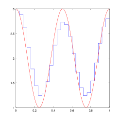
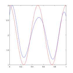
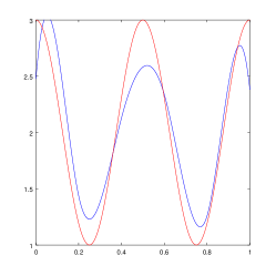
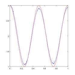
The setup is according to the theoretical study. We fix some function $x_{0}\colon[0,1]\to\mathbb{R}^{+}$, and then we generate data $y^{\delta}=F(x_{0})+\delta\xi$ on a fine grid (meshsize= $5000$), where $\|\xi\|_{\infty}=1$. For different values of $\delta=0.04,0.0025$ we let $\alpha=\sqrt{\delta}$. The theoretical results were based on the accretivity assumption, and we shall perform simulations, both for $x_{0}$ that satisfies (1) in Lemma 3, but also for $x_{0}$ violating the accretivity assumption for $\sigma=0$. The spaces $\tilde{X}_{m}$ are chosen both, as piece-wise constant functions, and cubic splines, respectively, and on a grid with discretization level $m\geq\lceil\frac{1}{\delta}\rceil$ for piece-wise constant functions and $m\geq\lceil\sqrt[4]{\frac{20}{\delta}}\rceil$ for cubic splines.

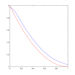
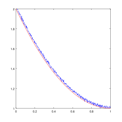
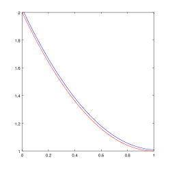
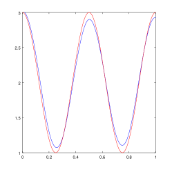
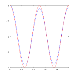
We then show the reconstructions, for piece-wise constant ansatz functions, without( left panel) and with (middle panel) post-smoothing by cubic spline interpolation. We add the corresponding reconstructions with cubic splines (right panel). For the first and the last case we obtain a convergence rate of order $\frac{1}{2}$ from the theory (cf. Theorem 1).

4.3. Accretivity for $\mathbf{\sigma=0}$

Here we let

(21) $$x_{0}(t)=t^{2}-2t+2,\quad 0\leq t\leq 1.$$

This function is positive, decreasing and convex on the unit interval, and hence $\sigma=0$ is appropriate for the accretivity. Figure 2 shows the reconstructions for the noise level $\delta=0.04$, whereas Figure 3 for $\delta=0.0025$.

Figure 2. Simulations for $\delta=0.04$

Figure 3. Simulations for $\delta=0.0025$

Table 1. computation times for function $x_{0}$ from (21)

data error	approximation space	$m$	cpu-time [s]
$\delta=0.0025$	piece-wise constant	$400$	$1.68$
	cubic splines	$10$	$1076$
$\delta=0.04$	piece-wise constant	$25$	$0.173$
	cubic splines	$5$	$338$

The computation times for the different methods are shown in Table 1. Since the time for smoothing the piece-wise constant solution is negligible, the corresponding computation times are not listed here.

Figure 4 shows a log-log plot of reconstruction errors of the different reconstruction methods depending on the noise level.

Figure 4. $-\ln(\|x_{\alpha}^{\delta}-x_{0}\|)$ versus $-\ln(\delta)$ for piece-wise constant (red), smoothed piece-wise constant (blue), and cubic splines (black) ansatz

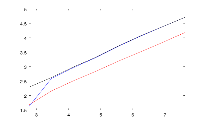
We observe that we obtain acceptable reconstructions from all three methods, where post smoothing of the piece-wise constant reconstruction and cubic spline ansatz yield almost identical results. Since the computation time for the piece-wise constant ansatz is much lower, we recommend this method. In Figure 4 we see that all three methods have a numerical convergence rate of approximately $\frac{1}{2}$, where the curves for the last two methods are almost identical for small data error.

4.4. Accretivity for positive $\sigma$

We consider the function

(22) $$x_{0}(t)=2+\cos(4\pi t),\quad 0\leq t\leq 1.$$

The following Figures 5 & 6, show the reconstructions.

Figure 5. Simulations for $\delta=0.04$

Figure 6. Simulations for $\delta=0.0025$

Table 2. computation times for function $x_{0}$ from (22)

data error	approximation space	$m$	cpu-time [s]
$\delta=0.0025$	piece-wise constant	$400$	$1.60$
	cubic splines	$10$	$1003$
$\delta=0.04$	piece-wise constant	$25$	$0.176$
	cubic splines	$5$	$319$

Figure 7. $-\ln(\|x_{\alpha}^{\delta}-x_{0}\|)$ versus $-\ln(\delta)$ for piece-wise constant (red), smoothed piece-wise constant (blue), and cubic splines (black) ansatz

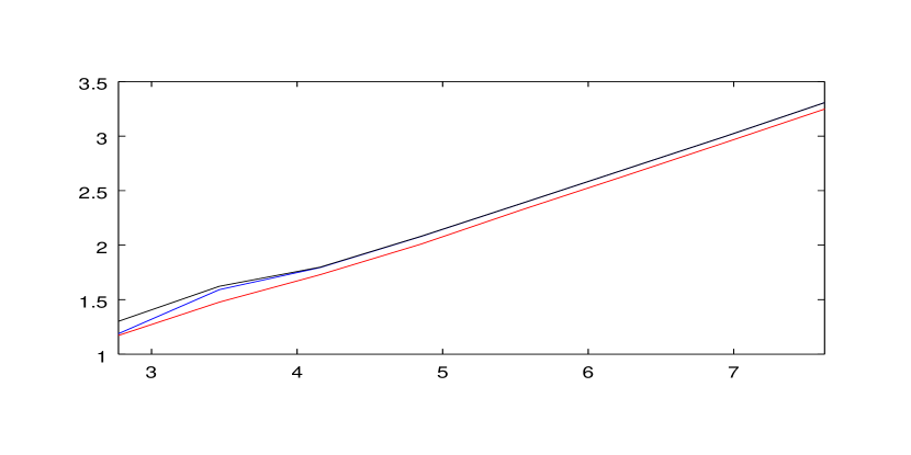
In principle we observe the same behavior as for the first test function. The numerical convergence rates shown in figures 7 are slightly lower than $\frac{1}{2}$. A reason could be that the constant $c$ in the parameter choice rule $\alpha=c\sqrt{\delta}$ has been chosen to small.

Appendix A Proofs

Proof of Lemma 1.

First, notice that the mappings $Q_{m}^{\sigma}$ are idempotent, and hence projections onto their ranges. Further we have the relation between the weighted and unweighted spaces

$$\|x\|_{\sigma}=\|D_{\sigma}^{-1}x\|,\qquad x\in L_{2}(0,1).$$

This yields

$$\left\|Q_{m}^{\sigma}x\right\|_{\sigma}=\left\|D_{\sigma}^{-1}Q_{m}^{\sigma}x\right\|=\left\|Q_{m}D_{\sigma}^{-1}x\right\|=\left\|D_{\sigma}^{-1}x\right\|=\left\|x\right\|_{\sigma},\ {x\in D_{\sigma}(X_{m})},$$

such that the mappings $Q_{m}^{\sigma}$ are partial isometries, and hence orthogonal projections on their ranges.

To show the approximation property let $x\in H_{1}(0,1)$ be arbitrary. Then $f_{\sigma}^{-1}x\in H_{1}(0,1)$ because $f_{\sigma}^{-1}$ is a smooth function. Since $Q_{m}$ satisfies assumption 3 we obtain

$$\|f_{\sigma}^{-1}x-Q_{m}(f_{\sigma}^{-1}x)\|\leq\frac{L}{m}\|f_{\sigma}^{-1}x\|_{H_{1}}.$$

Moreover we have

$$\|f_{\sigma}^{-1}x\|_{H_{1}}^{2} =\|f_{\sigma}^{-1}x\|^{2}+\|(f_{\sigma}^{-1}x)^{\prime}\|^{2}$$

$$=\|f_{\sigma}^{-1}x\|^{2}+\|-\sigma f_{\sigma}^{-1}x+f_{\sigma}^{-1}x^{\prime}\|^{2}$$

$$\leq(1+2\sigma^{2})\|f_{\sigma}^{-1}x\|^{2}+2\|f_{\sigma}^{-1}x^{\prime}\|^{2}$$

$$=(1+2\sigma^{2})\|x\|_{\sigma}^{2}+2\|x^{\prime}\|_{\sigma}^{2}$$

$$\leq\max\left\{2,1+2\sigma^{2}\right\}\|x\|_{H_{1}^{\sigma}}^{2}.$$

Using the above two estimates we derive

$$\|x-Q_{m}^{\sigma}x\|_{\sigma} =\|D_{\sigma}^{-1}x-D_{\sigma}^{-1}D_{\sigma}Q_{m}D_{\sigma}^{-1}x\|$$

$$=\|f_{\sigma}^{-1}x-Q_{m}(f_{\sigma}^{-1}x)\|$$

$$\leq\frac{L}{m}\|f_{\sigma}^{-1}x\|_{H_{1}}$$

$$\leq\max\left\{\sqrt{2},\sqrt{1+2\sigma^{2}}\right\}\frac{L}{m}\|x\|_{H_{1}^{\sigma}}.$$

Since we find that $\max\left\{\sqrt{2},\sqrt{1+2\sigma^{2}}\right\}\leq\sqrt{2}\left(1+\sigma\right)$ we can complete the proof. ∎

A.1. Proofs for § 2.3

Before turning to the proof of Proposition 1 we provide representations for $y_{0}$ and its derivatives. Indeed, since it holds $y_{0}(0)=0$, we have , from the Taylor expansion that

(23) $$y_{0}(s) =y_{0}(0)+y_{0}^{\prime}(0)s+\frac{1}{2}y_{0}^{\prime\prime}(\xi)s^{2}=y_{0}^{\prime}(0)s+\frac{1}{2}y_{0}^{\prime\prime}(\xi)s^{2}\,\text{ for some $\xi\in[0,s]$}$$

$$y_{0}^{\prime}(s) =x_{0}(0)x_{0}(s)+\int_{0}^{s}x_{0}^{\prime}(s-t)x_{0}(t)\mathrm{d}t=x_{0}(0)x_{0}(s)+\int_{0}^{s}x_{0}(s-t)x_{0}^{\prime}(t)\mathrm{d}t,$$

$$y_{0}^{\prime\prime}(s) =2x_{0}(0)x_{0}^{\prime}(s)+\int_{0}^{s}x_{0}^{\prime}(s-t)x_{0}^{\prime}(t)\mathrm{d}t.$$

This shows, among other things that $y^{\prime\prime}$ is continuous, but we also conclude that

(24) $$\left\|y_{0}^{\prime}\right\|_{\infty}\leq 2\left\|x_{0}\right\|_{C^{1}(0,1)}^{2}\quad\text{and}\quad\left\|y_{0}^{\prime\prime}\right\|_{\infty}\leq 3\left\|x_{0}\right\|_{C^{1}(0,1)}^{2}.$$

Proof of Proposition 1.

We first derive a uniform bound. We shall use the piece-wise constant approximations from Example 1. For $t\in\Delta$ we then find that

$$\left|(Q_{m}y_{0}-y_{0})(t)\right|=m\left|\int_{\Delta}(y_{0}(\tau)-y_{0}(t)\mathrm{d}\tau\right|,$$

which yields the bound

$$\left|(Q_{m}y_{0}-y_{0})(t)\right|\leq\frac{1}{m}\left\|y_{0}^{\prime}\right\|_{\infty},$$

by using $\left|y_{0}(\tau)-y_{0}(t)\right|=\left|y_{0}^{\prime}(\xi)(\tau-t)\right|\leq\left|\Delta\right|\left\|y_{0}^{\prime}\right\|_{\infty}$. Thus we have

(25) $$\left\|Q_{m}y_{0}-y_{0}\right\|_{\infty}\leq\frac{1}{m}\left\|y_{0}^{\prime}\right\|_{\infty}\leq\frac{2}{m}\left\|x_{0}\right\|_{C^{1}(0,1)}^{2},$$

by virtue of (24). Let now $h>0$. We start with (23) (s:=h), which yields for the derivative of $y_{0}$ at zero

$$y_{0}^{\prime}(0)=\frac{y_{0}(h)}{h}-\frac{1}{2}y_{0}^{\prime\prime}(\xi)h.$$

Using (1), (24) and (25) we see that

$$\left|\frac{[Q_{m}y^{\delta}](h)}{h}-y_{0}^{\prime}(0)\right| \leq\frac{|[Qy^{\delta}](h)-[Qy_{0}](h)|}{h}+\frac{|[Qy_{0}](h)-y_{0}(h)|}{h}$$

$$+\frac{1}{2}h|y_{0}^{\prime\prime}(\xi)|\leq\frac{\delta+\tfrac{2}{m}{\left\|x_{0}\right\|_{C^{1}(0,1)}^{2}}}{h}+\frac{3}{2}\left\|x_{0}\right\|_{C^{1}(0,1)}^{2}h,$$

If we set $h={\sqrt{\delta}}$ this yields

$$\left|\frac{1}{\sqrt{\delta}}{[Q_{m}y^{\delta}](\sqrt{\delta}})-y_{0}^{\prime}(0)\right| \leq\left(1+\frac{2\left\|x_{0}\right\|_{C^{1}(0,1)}^{2}}{m\delta}+\frac{3}{2}\left\|x_{0}\right\|_{C^{1}(0,1)}^{2}\right)\sqrt{\delta}$$

$$\leq\left(1+\frac{7}{2}\left\|x_{0}\right\|_{C^{1}(0,1)}^{2}\right)\sqrt{\delta},$$

provided that $m\delta\geq 1$. Since for $a,b>0$ it holds true that $\left|\sqrt{a}-b\right|\leq\tfrac{\left|a-b^{2}\right|}{b}$, whereas for $a<0$ we have $b\leq\frac{\left|a-b^{2}\right|}{b}$, we can complete the proof with letting

$$a:=\begin{cases}\sqrt{\frac{1}{\sqrt{\delta}}[Q_{m}y^{\delta}](\sqrt{\delta})},&\text{ if }[Q_{m}y^{\delta}](\sqrt{\delta})\geq 0,\\ 0,&\text{else}.\end{cases}$$

and $b:=x_{0}(0)$, such that $b^{2}=y_{0}^{\prime}(0)$, cf. the above representations for $y_{0}$ and its derivatives. ∎

Proof of Proposition 2.

Due to (23) we obtain

$$|y_{0}(t)-y_{0}^{\prime}(0)t|\leq\frac{1}{2}y_{0}(\xi)t^{2}\qquad\text{for some }\xi\in[0,t].$$

Using (24) this gives

$$|y_{0}(t)-y_{0}^{\prime}(0)t|\leq\frac{3}{2}\|x_{0}\|^{2}_{C^{1}(0,1)}t^{2}.$$

Integration from $0$ to $h$ yields

$$\left|\int_{0}^{h}y_{0}(t)\mathrm{d}t-\frac{1}{2}h^{2}y_{0}^{\prime}(0)\right|\leq\frac{1}{2}h^{3}\|x_{0}\|^{2}_{C^{1}(0,1)}.$$

Moreover, by the Hölder inequality we have

$$\left|\int_{0}^{h}(y_{0}(t)-y^{\delta}(t))\mathrm{d}t\right| \leq\int_{0}^{h}|y_{0}(t)-y^{\delta}(t)|\mathrm{d}t$$

$$\leq\sqrt{\int_{0}^{h}(y_{0}(t)-y^{\delta}(t))^{2}\mathrm{d}t}\cdot\sqrt{\int_{0}^{h}\mathrm{d}t}\leq\delta\sqrt{h}.$$

The triangle inequality yields

$$\left|\int_{0}^{h}y^{\delta}(t)\mathrm{d}t-\frac{1}{2}h^{2}y_{0}^{\prime}(0)\right|\leq\frac{1}{2}h^{3}\|x_{0}\|^{2}_{C^{1}(0,1)}+\delta\sqrt{h}$$

or equivalently

$$\left|\frac{2}{h^{2}}\int_{0}^{h}y^{\delta}(t)\mathrm{d}t-y_{0}^{\prime}(0)\right|\leq h\|x_{0}\|^{2}_{C^{1}(0,1)}+\delta h^{-\frac{3}{2}}.$$

Considered as a function of $h$, the right hand side of this inequality obtains its minimum for $h:=\left(\frac{2}{3}\|x_{0}\|^{2}_{C^{1}(0,1)}\right)^{-\frac{2}{5}}\delta^{\frac{2}{5}}$, and then the assertion is proved. ∎

A.2. Proofs for § 2.4

Proof of Proposition 3.

We recall the definition of the mapping $G$ from (15). We shall first see that there is some $r>0$ such that $\left\|Qx-x_{0}\right\|_{\sigma}\leq r$ yields that $\left\|G(Qx)-x_{0}\right\|_{\sigma}\leq r$. By the definition of $G$ we see that

$$\left\|G(Qx)-x_{0}\right\|_{\sigma}\leq I_{1}+I_{2}+I_{3}+I_{4},$$

where

$$I_{1} :=\|H_{\alpha}^{-1}QF^{\prime}(x_{0})(x_{0}-Qx_{0})\|_{\sigma},$$

$$I_{2} :=\|H_{\alpha}^{-1}Q(y^{\delta}-y)\|_{\sigma},$$

$$I_{3} :=\|H_{\alpha}^{-1}QF(Qx-x_{0})\|_{\sigma},\quad\text{and}$$

$$I_{4} :=\|H_{\alpha}^{-1}\alpha(Qx_{*}-x_{0})\|_{\sigma}.$$

We bound each summand, separately. By using Lemma 2 and Assumption 3 we find that

$$I_{1} \leq\left\|H_{\alpha}^{-1}\right\|_{\sigma}\left\|F^{\prime}(x_{0})\right\|_{\sigma}\left\|Qx_{0}-x_{0}\right\|_{\sigma}\leq\frac{2L}{m\alpha}\left\|x_{0}\right\|_{\sigma}\left\|x_{0}\right\|_{H_{1}^{\sigma}(0,1)}$$

$$\leq\frac{2L}{m\alpha}\left\|x_{0}\right\|_{H_{1}^{\sigma}(0,1)}^{2}\left\|Q\right\|_{\sigma\to\sigma}.$$

where throughout we use $\left\|Q\right\|_{\sigma\to\sigma}=1$, since $Q:L_{2}^{\sigma}(0,1)\to L_{2}^{\sigma}(0,1)$ is an orthogonal projection by Assumption 3. By Assumption 1(1) on the noise we bound

$$I_{2}\leq\|H_{\alpha}^{-1}\|_{\sigma}\,\|Q(y^{\delta}-y)\|_{\sigma}\leq\frac{\delta}{\alpha}.$$

Next, we see from Lemma 2 that

$$I_{3}\leq\|H_{\alpha}^{-1}\|_{\sigma}\,\|F(Qx-x_{0})\|_{\sigma}\leq\frac{\|Qx-x_{0}\|_{\sigma}^{2}}{\alpha}.$$

The bound for $I_{4}$ is more tedious, and we decompose

$$I_{4} \leq\alpha\|H_{\alpha}^{-1}(Q(x_{0}(0)-x_{0})+Q(x_{*}-x_{0}(0))+(Qx_{0}-x_{0})\|_{\sigma}$$

$$\leq\alpha\|H_{\alpha}^{-1}(Q(x_{0}(0)-x_{0}))\|_{\sigma}+\alpha\|H_{\alpha}^{-1}Q(x_{*}-x_{0}(0))\|_{\sigma}+\alpha\|H_{\alpha}^{-1}(Qx_{0}-x_{0})\|_{\sigma}.$$

Again, we bound separately. The last summand is easily bounded as

$$\alpha\|H_{\alpha}^{-1}(Qx_{0}-x_{0})\|_{\sigma}\leq\frac{L}{m}\left\|x_{0}\right\|_{H_{1}^{\sigma}}.$$

For the middle summand we recall that the reference element $x_{\ast}$ was chosen constant, cf. (13), such that by Proposition 1 we find

$$\alpha\|H_{\alpha}^{-1}Q(x_{*}-x_{0}(0))\|_{\sigma}\leq\|Q(x_{*}-x_{0}(0))\|_{\sigma}\leq\frac{\left(1+{4\left\|x_{0}\right\|_{C^{1}(0,1)}^{2}}\right)}{x_{0}(0)}\sqrt{\delta}.$$

It remains to bound the first summand in $I_{4}$, above. To this end we use the element $\omega$ from (11) and find that

$$\alpha\|H_{\alpha}^{-1}(Q(x_{0}(0)-x_{0}))\|_{\sigma}\leq\alpha\left\|H_{\alpha}^{-1}QF^{\prime}(x_{0})\omega\right\|_{\sigma}.$$

We bound the right hand side, again using Lemma 2, as

$$\alpha\left\|H_{\alpha}^{-1}QF^{\prime}(x_{0})\omega\right\|_{\sigma} \leq\alpha\left\|H_{\alpha}^{-1}QF^{\prime}(x_{0})Q\omega\right\|_{\sigma}+\alpha\left\|H_{\alpha}^{-1}QF^{\prime}(x_{0})(\operatorname{Id}-Q)\omega\right\|_{\sigma}$$

$$\leq\alpha\left\|\omega\right\|_{\sigma}+2\left\|Q\right\|_{\sigma\to\sigma}\left\|x_{0}\right\|_{\sigma}\left\|(\operatorname{Id}-Q)\omega\right\|_{\sigma}.$$

By Assumption 2 the right hand side in (11) is in $W_{\infty}^{2}(0,1)$, its derivative is in $H_{1}^{\sigma}$, and so will be the element $\omega$, where we refer to [7, Proof of Lem. 4]. Therefore Assumption 3 gives

$$\alpha\left\|H_{\alpha}^{-1}QF^{\prime}(x_{0})\omega\right\|_{\sigma}\leq\alpha\left(\left\|\omega\right\|_{\sigma}+\frac{2L}{m\alpha}\left\|Q\right\|_{\sigma\to\sigma}\left\|x_{0}\right\|_{\sigma}\left\|\omega\right\|_{H_{1}^{\sigma}(0,1)}\right).$$

Overall this gives for $I_{4}$ the bound

$$I_{4} \leq\alpha\left\|\omega\right\|_{\sigma}+$$

$$\frac{2L}{m}\left\|x_{0}\right\|_{\sigma}\left\|\omega\right\|_{H_{1}^{\sigma}(0,1)}+\frac{L}{m}\left\|x_{0}\right\|_{H_{1}^{\sigma}}+\frac{\left(1+{4\left\|x_{0}\right\|_{C^{1}(0,1)}^{2}}\right)}{x_{0}(0)}\sqrt{\delta}.$$

We rearrange terms and write

(26) $$\left\|G(Qx)-x_{0}\right\|_{\sigma}\leq I_{3}+\left(I_{1}+I_{2}+I_{4}\right).$$

The following result proves useful.

Lemma 5.

Suppose that $a,b,u,v\geq 0$ are such that $u\leq av^{2}+b$. If $4ab<1$ then $v\leq r$ implies that $u\leq r$ for the choice of

(27) $$r=\frac{1}{2a}\left(1-\sqrt{1-4ab}\right).$$

Proof.

The assertion holds true if $r$ can be found such that $ar^{2}-r+b\leq 0$, and this is the case whenever $4ab<1$. In this case the choice of $r$ according to (27) does the job. ∎

We shall apply this fact to the estimate (26), hence with $u:=\left\|G(Qx)-x_{0}\right\|_{\sigma},v:=\|Qx-x_{0}\|_{\sigma},a:=\alpha^{-1}\left\|Q\right\|_{\sigma\to\sigma},b:=I_{1}+I_{2}+I_{4}$. Thus, we aim at arranging the parameter $\alpha>0$ such that

$$4\alpha^{-1}\left\|Q\right\|_{\sigma\to\sigma}\left(I_{1}+I_{2}+I_{4}\right) =4\left\|Q\right\|_{\sigma\to\sigma}\left\|\omega\right\|_{\sigma}$$

$$+4\alpha^{-1}\left\|Q\right\|_{\sigma\to\sigma}\left(I_{1}+I_{2}+I_{4}-\alpha\left\|\omega\right\|_{\sigma}\right)<1.$$

The first summand is smaller than one under the assumption on $\left\|\omega\right\|_{\sigma}$, (note that $\|Q\|_{\sigma\to\sigma}=1$ here), and hence we need to make the second summand, temporarily denoted by $\operatorname{Res}$, sufficiently small for an appropriate choice of $\alpha$. Looking at the bounds for $I_{1},I_{2}$ and $I_{4}$ we find constants $C_{1},\dots,C_{5}>0$ such that

$$\operatorname{Res}\leq C_{1}\frac{1}{m\alpha^{2}}+C_{2}\frac{\delta}{\alpha^{2}}+C_{3}\frac{1}{m\alpha}+C_{4}\frac{\sqrt{\delta}}{\alpha}+C_{5}\frac{1}{m\alpha}.$$

Now we recall that the bounds were obtained under the assumption that $m\delta\geq 1$ (cf. Proposition 1), and assuming that the noise level is small, hence assuming that $\delta\leq 1$, then we can specify the previous bound to the form

$$\operatorname{Res}\leq\left(C_{1}+C_{2}\right)\frac{\delta}{\alpha^{2}}+\left(C_{3}+C_{4}+C_{5}\right)\sqrt{\frac{\delta}{\alpha^{2}}}.$$

Thus, the remainder $\operatorname{Res}$ can be made arbitrarily small if $\delta/\alpha^{2}$ is sufficiently small. This can be achieved by letting $\alpha:=c\sqrt{\delta}$ with a sufficiently large constant $c>0$.

Under the assumptions made, and in the light of Lemma 5 we can find $r>0$ such that

$$G(B(x_{0},r)\cap\mathcal{R}Q)\subset B(x_{0},r)\cap\mathcal{R}Q.$$

Notice, that the set $B(x_{0},r)\cap\mathcal{R}Q$ is compact and convex, such that the Schauder Fixed Point Theorem, cf. [4, Chapt. V.9], yields the existence of a fixed point of the continuous mapping $G$. ∎

Proof of Theorem 1.

Under the given assumptions, by Proposition 3 the equation (14) has a solution, say $x^{\delta}_{\alpha}$ in $X_{m}$ which satisfies $x^{\delta}_{\alpha}\in B(x_{0},r)$, where $r$ is given by Lemma 5, with $a,b$ specified, there. Obviously, we can bound $r\leq 1/(2a)$. The specification for $a$ was given as $a:=\left\|Q_{m}\right\|_{\sigma\to\sigma}/\alpha$, and it yields that $r\leq\alpha/(2\left\|Q_{m}\right\|_{\sigma\to\sigma})\leq\alpha/2$, such that with $\alpha=c\sqrt{\delta}$ (cf. proof of Proposition 3), we find

$$r\leq\alpha/2=\frac{c}{2}\sqrt{\delta}.$$

Notice, that the value of $c$ depends on the constants $C_{1},\dots,C_{5}$, only, and these were dependent on properties of $x_{0}$, but not on the noise level $\delta$. which completes the proof. ∎

A.3. Proofs for § 3

Proof of Lemma 4.

Let $x\in L_{2}(0,1)$ and $s\in[0,1)$. Then there exists $i\in\mathbb{N}$, s.t. $s\in[\frac{i-1}{m},\frac{i}{m})$. Using $\frac{\sigma}{m}\leq 1$ and the inequality

$$|e^{x}-1|\leq 2|x|\qquad\text{ for }|x|\leq 1$$

we estimate

$$\big{|}[(Q_{m}-Q_{m}^{\delta})x](s)\big{|} =m\left|\int_{\frac{i-1}{m}}^{\frac{i}{m}}x(t)\mathrm{d}t-e^{\sigma s}\int_{\frac{i-1}{m}}^{\frac{i}{m}}e^{-\sigma t}x(t)\mathrm{d}t\right|$$

$$=me^{\sigma s}\left|\int_{\frac{i-1}{m}}^{\frac{i}{m}}(e^{\sigma(t-s)}-1)e^{-\sigma t}x(t)\mathrm{d}t\right|$$

$$\leq me^{\sigma s}\int_{\frac{i-1}{m}}^{\frac{i}{m}}\left|e^{\sigma(t-s)}-1\right|\cdot\left|e^{-\sigma t}x(t)\right|\mathrm{d}t$$

$$\leq me^{\sigma s}\int_{\frac{i-1}{m}}^{\frac{i}{m}}2\left|\sigma(t-s)\right|\cdot\left|e^{-\sigma t}x(t)\right|\mathrm{d}t$$

$$\leq me^{\sigma s}\int_{\frac{i-1}{m}}^{\frac{i}{m}}2\frac{\sigma}{m}\left|e^{-\sigma t}x(t)\right|\mathrm{d}t$$

$$\leq 2\sigma e^{\sigma s}\left(\int_{\frac{i-1}{m}}^{\frac{i}{m}}e^{-2\sigma t}x(t)^{2}\mathrm{d}t\right)^{\frac{1}{2}}\sqrt{\frac{1}{m}},$$

where we used the Hölder inequality in the last step. Now we have

$$\|(Q_{m}-Q_{m}^{\delta})x\|_{\sigma}^{2} =\sum_{i=1}^{m}\int_{\frac{i-1}{m}}^{\frac{i}{m}}e^{-2\sigma s}\big{|}[(Q_{m}-Q_{m}^{\sigma})x](s)\big{|}^{2}\mathrm{d}s$$

$$\leq\sum_{i=1}^{m}\int_{\frac{i-1}{m}}^{\frac{i}{m}}\frac{4\sigma^{2}}{m}\left(\int_{\frac{i-1}{m}}^{\frac{i}{m}}e^{-2\sigma t}x(t)^{2}\mathrm{d}t\right)\mathrm{d}s$$

$$=\frac{4\sigma^{2}}{m^{2}}\int_{0}^{1}e^{-2\sigma t}x(t)^{2}\mathrm{d}t=\frac{4\sigma^{2}}{m^{2}}\|x\|_{\sigma}^{2}$$

and thus

$$\|Q_{m}-Q_{m}^{\sigma}\|_{\sigma\to\sigma}\leq\frac{2\sigma}{m},$$

which proves the first assertion. Finally, in operator norms we bound

$$\left\|Q_{m}\right\|_{\sigma\to\sigma}\leq\left\|Q_{m}-Q_{m}^{\sigma}\right\|_{\sigma\to\sigma}+\left\|Q_{m}^{\sigma}\right\|_{\sigma\to\sigma}\leq\frac{2\sigma}{m}+1,$$

which completes the proof of the lemma. ∎

Proof of Corollary 2.

Let $v\in L_{2}(0,1)$ be arbitrary. Then

$$\left\langle\left(Q_{m}F^{\prime}(x)Q_{m}+\tfrac{8\sigma\|x\|_{\sigma}}{m}\operatorname{Id}\right)v,v\right\rangle_{\sigma}$$

$$=\left\langle Q_{m}^{\sigma}F^{\prime}(x)Q_{m}^{\sigma}v,v\right\rangle_{\sigma}+\left\langle Q_{m}F^{\prime}(x)Q_{m}v,v\right\rangle_{\sigma}-\left\langle Q_{m}^{\sigma}F^{\prime}(x)Q_{m}^{\sigma}v,v\right\rangle_{\sigma}+\frac{8\sigma\|x\|_{\sigma}}{m}\|v\|_{\sigma}^{2}$$

$$\geq\left\langle(Q_{m}-Q_{m}^{\sigma})F^{\prime}(x)Q_{m}v,v\right\rangle_{\sigma}+\left\langle Q_{m}^{\sigma}F^{\prime}(x)(Q_{m}-Q_{m}^{\sigma})v,v\right\rangle_{\sigma}+\frac{8\sigma\|x\|_{\sigma}}{m}\|v\|_{\sigma}^{2}$$

$$\geq\frac{8\sigma\|x\|_{\sigma}}{m}\|v\|_{\sigma}^{2}-\|(Q_{m}-Q_{m}^{\sigma})F^{\prime}(x)Q_{m}v\|_{\sigma}\cdot\|v\|_{\sigma}-\|Q_{m}^{\sigma}F^{\prime}(x)(Q_{m}-Q_{m}^{\sigma})v\|_{\sigma}\cdot\|v\|_{\sigma}$$

$$\geq\frac{8\sigma\|x\|_{\sigma}}{m}\|v\|_{\sigma}^{2}-2\|Q_{m}-Q_{m}^{\sigma}\|_{\sigma\to\sigma}\cdot\|F^{\prime}(x)\|_{\sigma\to\sigma}\cdot\|v\|_{\sigma}^{2}.$$

Now we use Lemma 2 and Lemma 4 to see that

$$2\|Q_{m}-Q_{m}^{\sigma}\|_{\sigma\to\sigma}\cdot\|F^{\prime}(x)\|_{\sigma\to\sigma}\cdot\|v\|_{\sigma}^{2}\leq\frac{8\sigma}{m}\left\|x\right\|_{\sigma}\left\|v\right\|_{\sigma}^{2},$$

which implies the accretivity of $Q_{m}F^{\prime}(x)Q_{m}+\frac{8\sigma\|x\|}{m}\operatorname{Id}$. For the sake of readability we set $J:=Q_{m}F^{\prime}(x)Q_{m}$. Let now $\alpha\geq\frac{16\sigma\|x\|}{m}$. Then $\frac{\alpha}{2}\geq\frac{8\sigma\|x\|}{m}$, thus $G:=J+\frac{\alpha}{2}\operatorname{Id}$ is accretive. We recall [7, Eq. (14)], which asserts that for $\beta>0$ we have

$$\|(\beta\operatorname{Id}+G)^{-1}\|_{\sigma}\leq\frac{1}{\beta}\quad\text{and}\quad\|(\beta\operatorname{Id}+G)^{-1}G\|_{\sigma}\leq 1.$$

We use this to conclude that

$$\|(\alpha\operatorname{Id}+J)^{-1}\|_{\sigma}=\|\big{(}\tfrac{\alpha}{2}\operatorname{Id}+(\tfrac{\alpha}{2}\operatorname{Id}+J)\big{)}^{-1}\|_{\sigma}\leq\frac{2}{\alpha},$$

and

$$\| (\alpha\operatorname{Id}+J)^{-1}J\|_{\sigma}=\|\big{(}\tfrac{\alpha}{2}\operatorname{Id}+(\tfrac{\alpha}{2}\operatorname{Id}+J)\big{)}^{-1}(\tfrac{\alpha}{2}\operatorname{Id}+J-\tfrac{\alpha}{2}\operatorname{Id})\|_{\sigma}$$

$$\leq\|\big{(}\tfrac{\alpha}{2}\operatorname{Id}+(\tfrac{\alpha}{2}\operatorname{Id}+J)\big{)}^{-1}(\tfrac{\alpha}{2}\operatorname{Id}+J)\|_{\sigma}+\|\big{(}\tfrac{\alpha}{2}\operatorname{Id}+(\tfrac{\alpha}{2}\operatorname{Id}+J)\big{)}^{-1}\tfrac{\alpha}{2}\operatorname{Id}\|_{\sigma}$$

$$\leq 1+\frac{2}{\alpha}\cdot\frac{\alpha}{2}=2,$$

and the proof is complete. ∎

Sketch of the proof of Proposition 4.

By Lemma 3, it exists a $\sigma_{1}>0$ s.t.

$$\|\omega\|_{\sigma_{1}}<\frac{1}{48}.$$

Since by Lemma 4 we have with $m\geq{\sigma_{1}}$ that

$$\|Q_{m}\|_{\sigma_{1}\to\sigma_{1}}\leq 1+2\frac{\sigma_{1}}{m}\leq 3$$

and hence we find that

$$\|\omega\|_{\sigma_{1}}\cdot\|Q_{m}\|_{\sigma_{1}\to\sigma_{1}}<\frac{1}{16}.$$

In the following we will abbreviate $Q_{m}$ by $Q$. Basically we follow the proofs of Proposition 3 and Theorem 1, but the norm $\left\|Q\right\|_{\sigma\to\sigma}$ is no longer equal to one. Analogous to (15) we write equation (17) in fix-point form as

$$G(Qx)=Qx$$

with

$$G(Qx):=x_{0}+H_{\alpha}^{-1}\Big{(}Q\big{(}F^{\prime}(x_{0})(x_{0}-Qx_{0})+y^{\delta}-y-F(Q_{m}x-x_{0})\big{)}+\alpha(Qx_{*}-x_{0})\Big{)},$$

where

$$H_{\alpha}:=QF^{\prime}(x_{0})Q.$$

As in the proof of Prop. 3 we have

$$\left\|G(Qx)-x_{0}\right\|_{\sigma_{1}}\leq I_{1}+I_{2}+I_{3}+I_{4},$$

where

$$I_{1} :=\|H_{\alpha}^{-1}QF^{\prime}(x_{0})(x_{0}-Qx_{0})\|_{\sigma_{1}},$$

$$I_{2} :=\|H_{\alpha}^{-1}Q(y^{\delta}-y)\|_{\sigma_{1}},$$

$$I_{3} :=\|H_{\alpha}^{-1}QF(Qx-x_{0})\|_{\sigma_{1}}\quad\text{and}$$

$$I_{4} :=\|H_{\alpha}^{-1}\alpha(Qx_{*}-x_{0})\|_{\sigma_{1}}.$$

The following estimations are almost the same as before, except that we assume

(28) $$\alpha\geq\frac{16\sigma\|x\|}{m}$$

and make use of Corollary 2. This yields

$$I_{1} \leq\frac{4L}{m\alpha}\left\|x_{0}\right\|_{H_{1}^{\sigma_{1}}(0,1)}^{2}\left\|Q\right\|_{\sigma_{1}\to\sigma_{1}},$$

$$I_{2} \leq 2\frac{\delta}{\alpha}\left\|Q\right\|_{\sigma_{1}\to\sigma_{1}},$$

$$I_{3} \leq 2\frac{\|Qx-x_{0}\|_{\sigma_{1}}^{2}}{\alpha}\left\|Q\right\|_{\sigma_{1}\to\sigma_{1}}$$

and

$$I_{4} \leq 2\alpha\left\|\omega\right\|_{\sigma_{1}}+\frac{4L}{m}\left\|Q\right\|_{\sigma_{1}\to\sigma_{1}}\left\|x_{0}\right\|_{\sigma_{1}}\left\|\omega\right\|_{H_{1}^{\sigma_{1}}(0,1)}$$

$$+\frac{2L}{m}\left\|x_{0}\right\|_{H_{1}^{\sigma_{1}}}+\frac{2\left(1+{4\left\|x_{0}\right\|_{C^{1}(0,1)}^{2}}\right)}{x_{0}(0)}\sqrt{\delta}\left\|Q\right\|_{\sigma_{1}\to\sigma_{1}}.$$

Now we want to apply Lemma 5 with the parameters $u:=\left\|G(Qx)-x_{0}\right\|_{\sigma_{1}},v:=\|Qx-x_{0}\|_{\sigma_{1}},a:=2\alpha^{-1}\left\|Q\right\|_{\sigma_{1}\to\sigma_{1}},b:=I_{1}+I_{2}+I_{4}$. Again we have to ensure that $4ab<1$. This is equivalent to

$$16\left\|Q\right\|_{\sigma_{1}\to\sigma_{1}}\left\|\omega\right\|_{\sigma_{1}}+8\alpha^{-1}\left\|Q\right\|_{\sigma_{1}\to\sigma_{1}}\left(I_{1}+I_{2}+I_{4}-2\alpha\left\|\omega\right\|_{\sigma_{1}}\right)<1.$$

Due to the choice of $\sigma_{1}$ we have

$$16\left\|Q\right\|_{\sigma_{1}\to\sigma_{1}}\left\|\omega\right\|_{\sigma_{1}}<1$$

and the second summand, denoted by $\operatorname{Res}$ can be estimated as

$$\operatorname{Res}\leq C_{1}\frac{1}{m\alpha^{2}}+C_{2}\frac{\delta}{\alpha^{2}}+C_{3}\frac{1}{m\alpha}+C_{4}\frac{\sqrt{\delta}}{\alpha}+C_{5}\frac{1}{m\alpha}.$$

with constants $C_{1},\dots,C_{5}$. With the assumptions $m\delta\geq 1$ and $\delta\leq 1$ we derive

$$\operatorname{Res}\leq\left(C_{1}+C_{2}\right)\frac{\delta}{\alpha^{2}}+\left(C_{3}+C_{4}+C_{5}\right)\sqrt{\frac{\delta}{\alpha^{2}}}.$$

Hence $\operatorname{Res}$ can be made arbitrarily small by setting $\alpha=c\sqrt{\delta}$ with $c$ big enough and $c\geq\frac{16\sigma\|x\|}{m\sqrt{\delta}}$, which ensures (28). If $c$ is now chosen in such a way that

$$16\left\|Q\right\|_{\sigma_{1}\to\sigma_{1}}\left\|\omega\right\|_{\sigma_{1}}+\operatorname{Res}<1$$

we apply Lemma 5 and obtain

$$G(B(x_{0},r)\cap\mathcal{R}Q)\subset B(x_{0},r)\cap\mathcal{R}Q.$$

for $r=\frac{1}{2a}\left(1-\sqrt{1-4ab}\right)$. Since $B(x_{0},r)\cap\mathcal{R}Q$ is a compact and convex set, we obtain that $G$ has a fixed point by the Schauder Fixed Point Theorem. The remainder of the proof is analogous to the proof of Theorem 1. ∎

References

- [1] Stephan W Anzengruber, Steven Bürger, Bernd Hofmann, and Günter Steinmeyer. Variational regularization of complex deautoconvolution and phase retrieval in ultrashort laser pulse characterization. Inverse Problems, 32(3):035002, 2016.
- [2] Steven Bürger and Jens Flemming. Deautoconvolution: a new decomposition approach versus TIGRA and local regularization. J. Inverse Ill-Posed Probl., 23(3):231–243, 2015.
- [3] Steven Bürger and Bernd Hofmann. About a deficit in low-order convergence rates on the example of autoconvolution. Appl. Anal., 94(3):477–493, 2015.
- [4] John B. Conway. A course in functional analysis, volume 96 of Graduate Texts in Mathematics. Springer-Verlag, New York, second edition, 1990.
- [5] Gunter Fleischer and Bernd Hofmann. On inversion rates for the autoconvolution equation. Inverse Problems, 12(4):419–435, 1996.
- [6] Rudolf Gorenflo and Bernd Hofmann. On autoconvolution and regularization. Inverse Problems, 10(2):353–373, 1994.
- [7] Jaan Janno. Lavrent′ev regularization of ill-posed problems containing nonlinear near-to-monotone operators with application to autoconvolution equation. Inverse Problems, 16(2):333–348, 2000.
- [8] Shuai Lu, Valeriya Naumova, and Sergei V. Pereverzev. Legendre polynomials as a recommended basis for numerical differentiation in the presence of stochastic white noise. J. Inverse Ill-Posed Probl., 21(2):193–216, 2013.
- [9] Shuai Lu and Sergei V. Pereverzev. Numerical differentiation from a viewpoint of regularization theory. Math. Comp., 75(256):1853–1870, 2006.
- [10] K.-Th. Schleicher, S.W. Schulz, R. Gmeiner, and H.-U. Chun. A computational method for the evaluation of highly resolved dos functions from APS measurements. Journal of Electron Spectroscopy and Related Phenomena, 31(1):33 – 56, 1983.
- [11] Larry L. Schumaker. Spline functions: basic theory. Cambridge Mathematical Library. Cambridge University Press, Cambridge, third edition, 2007.