Spectral stability for classical periodic waves of the Ostrovsky and short pulse models

Abstract.

We consider the Ostrovsky and short pulse models in a symmetric spatial interval, subject to periodic boundary conditions. For the Ostrovsky case, we revisit the classical periodic traveling waves and for the short pulse model, we explicitly construct traveling waves in terms of Jacobi elliptic functions. For both examples, we show spectral stability, for all values of the parameters. This is achieved by studying the non-standard eigenvalue problems in the form $Lu=\lambda u^{\prime}$, where $L$ is a Hill operator.

1. Introduction

The (generalized) Korteweg-De Vries equation

(1) $$u_{t}+\beta u_{xxx}+(f(u))_{x}=0,$$

is a basic model in the theory of water waves. In fact, this is one of the most ubiquitous models in the theory of partial differential equations, modeling the unidirectional motion of waves in shallow water. Its Cauchy problem has been comprehensively studied in the last 50 years. Our interest is in a related model, which takes into account the effect of a (small) rotation force acting on the fluid. More specifically,

(2) $$(u_{t}+\beta u_{xxx}+(f(u))_{x})_{x}=\epsilon u,-L\leq x\leq L.$$

Note that we consider (2) on a finite nterval, with periodic boundary conditions. The problem on the whole line case certainly makes sense physically, as an approximation of situations where the motion takes place on long intervals. We will however only consider the periodic case henceforth.

We refer to (2) as the regularized short pulse equation (RSPE), when $\beta\neq 0$. In [12, 13] the authors have constructed traveling wave solutions of (2) on the whole line by employing variational methods. They have also studied the stability of such solutions by following the Grillakis-Shatah-Strauss arguments. Further results on the stability of these traveling waves were obtained in [14, 15]. In [2], the authors have constructed pulse solutions of (2), for small values of $\epsilon$, via singular perturbation theory. In [3], they have shown the existence of multi-pulse solutions. The stability of these waves remains an interesting open problem.

An interesting special model occurs in the absence of a KdV regularization - in other words, $\beta=0$. This is referred to in the literature, depending on the form of the non-linearity $f$, as the reduced Ostrovsky or Ostrovsky-Hunter or short pulse model. Namely, after scaling all parameters to one, we have

(3) $$(u_{t}+(f(u))_{x})_{x}=u.$$

The model (3), with various form of the nonlinearity has rich history, most of it unrelated to the its connections to KdV. Ostrovsky, [19] in the late 70’s has introduced the first model of this sort. In the early 90’s, Vakhnenko, [24] proposed an alternative derivation, while Hunter, [11] proposed some numerical simulations. The well-posedness questions were investigated by Boyd, [1]; Schaefer and Wayne, [21]; Stefanov-Shen-Kevrekidis, [22]. Liu, Pelinovsky and Sakovich, [16, 17] have studied wave breaking, which was later supplemented by the global regularity results for small, in appropriate sense data, of Grimshaw-Pelinovsky, [7]. There are numerous works on explicit traveling wave solutions of these models, [6, 18, 20, 23, 25, 26]. One should note that some of this solutions are not classical solutions, but rather a multi-valued ones, [20]. Several authors have also explored the integrability of the Ostrovsky equation, [20, 26]. In particular, they have managed to construct the traveling waves by means of the inverse scattering transform. In this regard, it is worth mentioning the very recent work [10], where the authors study small periodic waves of the quadratic and cubic models in the form (3). They show orbital stability of such waves (with respect to all subharmonic perturbations!) by adapting the methods of [4] for periodic waves of the defocussing cubic NLS. Their proof makes sense of a representation of these waves as unconstrained minimizers of appropriate functionals. Another recent development in the area is our recent paper, [8], which gives an explicit construction of peakon type solutions and establishes their stability.

Our main interest in this paper is the stability of explicit traveling waves for the short pulse equation (3). More precisely, we follow the recent work of [6], who construct the solutions of (3), for $f(u)=u^{2}$, in terms of Jacobi elliptic functions, after a (solution dependent) change of variables. We consider these solutions and we show their spectral stability with respect to co-periodic perturbations ( i.e. with respect of perturbations of the same period). In addition, we construct a family of explicit solutions in the cubic case as well. Their spectral stability for co-periodic perturbations is established as well. In all our considerations, we consider the linearized problems after the change of variables, where we get eigenvalue problems in the form

(4) $$\mathcal{L}u=\mu u^{\prime}.$$

where $\mathcal{L}$ is a second order Hill operator, subject to periodic boundary conditions. Clearly, (4) is a non-standard eigenvalue problem, for which we develop appropriate methods to study its stability.

We now continue on to derive the profile equations and the linearized equations.

1.1. Profile equation and the linearized problem

As we have alluded above, we consider (3) with quadratic and cubic non-linearity. Even though, one can mostly proceed to derive the profile equation with the general non-linearity $f(u)$, we prefer to use the explicit form in the two cases, since the specific, solution dependent transformation (see [6]), depends in a significant way on the particular form of $f$.

1.1.1. The quadratic model

In order to derive the profile equations, we follow the approach of [6]. Our first consideration is the quadratic model $f(u)=\frac{u^{2}}{2}$, the so-called Ostrovsky equation. It reads

(5) $$(u_{t}+uu_{x})_{x}=u,\ \ -L\leq x\leq L.$$

Using the traveling wave ansatz, $u(t,x)=\varphi(x-ct)$, for an unknown periodic function $\varphi$, we arrive at the ODE,

(6) $$((\varphi-c)\varphi_{\xi})_{\xi}=\varphi\ \ -L\leq\xi\leq L.$$

Clearly, (6), being a fully nonlinear equation, is not a very nice object to deal with. Thus, we perform a (solution dependent) change of variables, namely

(7) $$\xi=\Xi(\eta):=\eta-\frac{\Psi(\eta)}{c},\ \ \varphi(\xi)=\Phi(\eta)=\Psi^{\prime}(\eta).$$

If $\varphi$ is an even function, so is $\Phi$ and then naturally $\Psi$ is an odd function. Compute

(8) $$\frac{d\Xi}{d\eta}=1-\frac{\Psi^{\prime}(\eta)}{c}=1-\frac{\varphi(\xi)}{c},$$

so that

$$\varphi_{\xi}=\frac{\Phi_{\eta}}{\frac{d\Xi}{d\eta}}=\frac{c\Phi_{\eta}}{c-\varphi(\xi)}.$$

Thus, $(\varphi-c)\varphi_{\xi}=-c\Phi_{\eta}$. Taking another derivative in $\xi$,

$$\Phi(\eta)=\varphi(\xi)=((\varphi-c)\varphi_{\xi})_{\xi}=-\frac{c^{2}\Phi_{\eta\eta}}{c-\varphi(\xi)}=-\frac{c^{2}\Phi_{\eta\eta}}{c-\Phi(\eta)}.$$

We are thus lead to the profile equation

(9) $$c^{2}\Phi^{\prime\prime}=\Phi(\Phi-c).$$

Clearly, (9) is a standard Schrödinger equation, which is much easier to study. We do so in Section 2 below, where an explicit expression for $\Phi$ is found. One has to keep in mind however, that the solutions of (9) are equivalent, so long as the transformation (7) is invertible. This is clearly requiring that the function $\eta\to\Xi(\eta)$ is monotone or equivalently, from (8), that either $\varphi(\xi)>c$ for each $\xi\in[-L,L]$ or $\varphi(\xi)<c$ for each $\xi\in[-L,L]$. If that is the case, we have an interval $[-M,M]$, so that $\Xi:[-M,M]\to[-L,L]$ is a diffeomorphism and the profile equation (9) has to be considered with periodic boundary conditions on $[-M,M]$.

Our next task is to derive the linearized problem for such solutions $\varphi$ - assuming that they exist and the transformation (7) is invertible in the appropriate interval. To this end, we take the ansatz $u(t,x)=\varphi(x-ct)+v(t,x-ct)$ in (5) and ignore all quadratic terms. We obtain the following linearized equation

(10) $$(v_{t}+((\varphi-c)v)_{\xi})_{\xi}=v\ \ -L<\xi<L.$$

Next, we turn (10) into an eigenvalue problem, by letting $v(t,\xi)=e^{\lambda t}w(\xi),w\in H^{2}[-L,L]$. This results in

(11) $$(\lambda w+((\varphi-c)w)_{\xi})_{\xi}=w\ \ -L<\xi<L.$$

Note that (11) guarantees that $w$ is an exact derivative, which justifies our next change of variables $w=z_{\xi}$. Here, we can assume that $z\in H^{3}(-L,L):\int_{-L}^{L}z(x)dx=0$. This can be of course always be achieved and in fact, it fixes the function $z$. Thus, we reduce matters to

$$(\lambda z_{\xi}+((\varphi-c)z_{\xi})_{\xi})_{\xi}=z_{\xi}\ \ -L<\xi<L.$$

An integration in $\xi$ (and taking into account that $\int_{-L}^{L}z(x)dx=0$) allows us to transform the last equation into the equivalent one

(12) $$\lambda z_{\xi}+((\varphi-c)z_{\xi})_{\xi}=z\ \ -L<\xi<L.$$

Indeed, in the last equation, the constant of integration is zero, since we have an exact derivative on the left-hand side and a function of mean value zero on the right-hand side.

Now, assume that there is an interval $[-M,M]$, so that $\Xi:[-M,M]\to[-L,L]$ is a diffeomorphism. This appeared previously as a necessary condition for the wave $\varphi$ to exists. Denote the inverse function of $\Xi$ by $\eta(\xi)$, that is $\xi=\Xi(\eta(\xi))$. Introduce $Z\in L^{2}(-M,M)$, so that $z(\xi)=Z(\eta(\xi))$. We have

$$z_{\xi}(\xi)=\frac{Z_{\eta}}{\frac{d\xi}{d\eta}}=\frac{Z_{\eta}}{1-\frac{\varphi(\xi)}{c}}=\frac{cZ_{\eta}}{c-\varphi(\xi)}.$$

Thus, $(c-\varphi(\xi))z_{\xi}=cZ_{\eta}$ and hence

$$[(c-\varphi)z_{\xi}]_{\xi}=c\frac{d}{d\xi}(Z_{\eta}(\eta(\xi)))=c\frac{Z_{\eta\eta}}{\frac{d\xi}{d\eta}}=\frac{c^{2}Z_{\eta\eta}}{c-\varphi(\xi)}=\frac{c^{2}Z_{\eta\eta}}{c-\Phi(\eta)}$$

Plugging the result in (12), we obtain

$$\frac{c^{2}Z_{\eta\eta}}{c-\Phi(\eta)}=[(c-\varphi)z_{\xi}]_{\xi}=\lambda z_{\xi}-z=\lambda\frac{cZ_{\eta}}{c-\Phi}-Z.$$

All in all, we obtain the eigenvalue problem,

(13) $$-c^{2}Z_{\eta\eta}-cZ+\Phi Z=-\lambda cZ_{\eta},Z\in L^{2}(-M,M).$$

1.1.2. The cubic model

For the cubic model, we follow an identical approach, with just a slight changes to reflect the cubic nonlinearity. More precisely, let $f(u)=\frac{u^{3}}{3}$. The profile equation for the traveling wave solution $\varphi(x-ct)$ is

(14) $$((\varphi^{2}-c)\varphi_{\xi})_{\xi}=\varphi,\ \ -L<\xi<L.$$

Next, the change of variables is of course in the form

(15) $$\Xi(\eta)=\eta-\frac{\Psi(\eta)}{c},\varphi(\xi)=\Phi(\eta),\Psi^{\prime}(\eta)=\Phi^{2}(\eta)=\varphi^{2}(\xi).$$

Again, if $\varphi$ and $\Phi$ are odd functions, then so is $\Psi$. Similar to the quadratic case, we have $(\varphi^{2}-c)\varphi_{\xi}=-c\Phi_{\eta},$ whence

$$\Phi(\eta)=\varphi(\xi)=((\varphi^{2}-c)\varphi_{\xi})_{\xi}=-\frac{c^{2}\Phi_{\eta\eta}}{c-\varphi^{2}(\xi)}=-\frac{c^{2}\Phi_{\eta\eta}}{c-\Phi^{2}(\eta)}.$$

Thus, we have the profile equation in the form

(16) $$-c^{2}\Phi_{\eta\eta}-c\Phi+\Phi^{3}=0.$$

Assuming that there is an interval $[-M,M]$, so that $\Xi:[-M,M]\to[-L,L]$ is a diffeomorphism, we can consider the profile equation (16) with periodic boundary conditions on $[-M,M]$.

We now discuss the linearization around the wave $\varphi(x-ct)$ for the model $(u_{t}+u^{2}u_{x})_{x}=u$. Following the same steps as in the quadratic case, with $\Xi$ defined as in (15), we arrive at the following linearized problem

(17) $$-c^{2}Z_{\eta\eta}-cZ+\Phi^{2}Z=-\lambda cZ_{\eta},Z\in L^{2}(-M,M).$$

1.1.3. Definition of spectral stability and plan of the paper

Now that we have introduced the profile equations and the linearized problems, it is time to formally introduce the definition of stability. For instability we require that (12) has a non-trivial solution $Z$ for some $\lambda:\Re\lambda>0$. One can easily see that if $\lambda$ (and some $Z$) is a solution of (13) or (17), then $(-\lambda,Z(-\cdot))$ is also a solution. That is, there is the spectral invariance $\lambda\to-\lambda$. Thus, instability means that there is a solution of (13) (or (17)) with right hand-side $\mu=-\lambda c>0$. If such a solution does not exist, we say that we have stability. Formally,

Definition 1.

Assume that the periodic wave $\varphi$ is a solution of (6), with some $c\neq 0$. Assume also that there exists a one-to-one mapping $\Xi:(-M,M)\to(-L,L),M\in(0,\infty]$ satisfying (7). We say the the wave is spectrally unstable, if there exists $\mu:\Re\mu>0$ and a function $Z\in H^{2}[-M,M]\cap C^{2}(-M,M)$, so that

(18) $$L[Z]:=-c^{2}Z_{\eta\eta}-cZ+\Phi Z=\mu Z^{\prime}.$$

Similarly, the solution $\varphi$ of (14) is unstable, if there is $\mu:\Re\mu>0$ and $Z\in H^{2}[-M,M]\cap C^{2}(-M,M)$, so that

(19) $$L[Z]:=-c^{2}Z_{\eta\eta}-cZ+\Phi^{2}Z=\mu Z^{\prime}.$$

The paper is organized as follows. In Section 2 we first revisit the construction of the even traveling waves for the Ostrovsky model and the odd solutions for the short pulse equation. Toward the end of Section 2, appropriate spectral information for the corresponding Hill operators is supplied as well. In Section 3, we develop, for the purposes of the subsequent sections, sufficient conditions for the positivity of a given self-adjoint operator (with finitely many negative eigenvalues) on a subspace of finite co-dimension. In Section 4, we consider the spectral stability of the waves in the quadratic (Ostrovsky) case. In Section 5, we discuss the spectral stability in the cubic (short pulse) case. Finally, in Section 6, we discuss the parabolic peakons for the Ostrovsky model, which can be seen as a limiting case of the waves constructed previously. We show, that the corresponding eigenvalue problem has smooth solutions inside the interval of consideration (which however do not satisfy any periodic boundary conditions).

2. Construction of the periodic waves and the spectral properties of the Hill operators

We first discuss the construction of periodic solutions in the case of quadratic nonlinearities.

2.1. Quadratic nonlinearities

Integrating once the equation (9), we get

(20) $$\Phi_{\eta}^{2}=\frac{2}{3c^{2}}\left[\Phi^{3}-\frac{3c}{2}\Phi^{2}+A\right]=F(\Phi),$$

where $A$ is a constant of integration. For $c<0$, in the phase plane $(\Phi,\Phi^{\prime})$ equation (9) has equilibra at $(0,0)$ which is saddle point and at $\left(c,0\right)$ which is a center. For $c>0$, in the phase plane $(\Phi,\Phi^{\prime})$ equation (9) has equilibra at $(c,0)$ which is saddle point and at $\left(0,0\right)$ which is a center.

Let $\Phi_{0}<\Phi_{1}<\Phi_{2}$ are roots of polynomial $F(\Phi)$. We have

(21) $$\left|\begin{array}[]{ll}\Phi_{0}+\Phi_{1}+\Phi_{2}=\frac{3c}{2}\\ \\ \Phi_{0}\Phi_{1}+\Phi_{0}\Phi_{2}+\Phi_{1}\Phi_{2}=0.\end{array}\right.$$

Introducing a new variable $s\in(0,1)$ via $\Phi=\Phi_{0}+(\Phi_{1}-\Phi_{0})s^{2}$, we transform (20) into

$$s^{\prime 2}=\alpha^{2}(1-s^{2})(1-k^{2}s^{2})$$

where $\alpha$ and $k$ are positive constants given by

(22) $$\alpha^{2}=\frac{\frac{3c}{2}-\Phi_{1}-2\Phi_{0}}{6c^{2}},\quad k^{2}=\frac{\Phi_{1}-\Phi_{0}}{\frac{3c}{2}-\Phi_{1}-2\Phi_{0}}.$$

Therefore

(23) $$\Phi=\Phi_{0}+(\Phi_{1}-\Phi_{0})sn^{2}(\alpha x;\kappa).$$

From (21) and (22, we have

(24) $$\left|\begin{array}[]{ll}\Phi_{1}-\Phi_{0}=6c^{2}\alpha^{2}\kappa^{2}\\ \\ \Phi_{0}=\frac{c}{2}-2c^{2}\alpha^{2}(1+\kappa^{2})\\ \\ \Phi_{1}=\frac{c}{2}+2c^{2}\alpha^{2}(2\kappa^{2}-1)\\ \\ 16c^{2}\alpha^{4}(1-\kappa^{2}+\kappa^{4})=1.\end{array}\right.$$

For $c>0$, from (23) and (24), and using that $sn^{2}(x)+cn^{2}(x)=1$, we have

$$1-\frac{\varphi(\xi)}{c}=2\alpha^{2}c(1-2\kappa^{2}+\sqrt{1-\kappa^{2}+\kappa^{4}}+3cn^{2}(\alpha\xi;\kappa))>0$$

With this we verified that the function defined in (7) is one-to-one.

2.2. Cubic nonlinearities

Here we need periodic solutions of (16). Integrating once the equation (16), we get

(25) $$\Phi_{\eta}^{2}=\frac{1}{2c^{2}}\left[\Phi^{4}-2c\Phi^{2}+A\right]=F(\Phi),$$

where $A$ is a constant of integration. Suppose that the polynomial $\rho^{4}-2c\rho^{2}+A$ has two positive roots $\Phi_{1}>\Phi_{2}>0$. Then, the equation (25) can be written in the form

(26) $$\Phi_{\eta}^{2}=\frac{1}{2c^{2}}(\Phi^{2}-\Phi_{1}^{2})(\Phi-\Phi_{2}^{2}).$$

Then the solution of the equation (26) is given by

(27) $$\Phi(x)=\Phi_{2}sn(\alpha x,\kappa),$$

where $-\Phi_{2}<\Phi(x)<\Phi_{2}$ and

(28) $$\left|\begin{array}[]{ll}\Phi_{1}^{2}+\Phi_{2}^{2}=2c\\ \\ \Phi_{1}^{2}\Phi_{2}^{2}=A\\ \\ \kappa^{2}=\frac{\Phi_{2}^{2}}{\Phi_{1}^{2}},\;\;\alpha=\frac{\Phi_{1}}{\sqrt{2}c}.\end{array}\right.$$

Note that from (28), $2c=\Phi_{1}^{2}+\Phi_{2}^{2}>2\Phi_{2}^{2}$, whence we have

(29) $$\Phi^{2}-c<\Phi^{2}_{2}-c^{2}<0$$

2.3. Quadratic nonlinearities: spectral properties of the Hill operator

For the operator

$$L=-c^{2}\partial_{x}^{2}-c+\Phi,$$

we have the representation $c=\frac{1}{4\alpha^{2}\sqrt{1-\kappa^{2}+\kappa^{4}}}>0$ and

(30) $$L=c^{2}\alpha^{2}(-\partial_{y}^{2}+6k^{2}sn^{2}(y,k)-2(1+k^{2}+\sqrt{1-k^{2}+k^{4}})).$$

It is well-known [9] that the first three eigenvalues of $\Lambda_{1}=-\partial_{y}^{2}+6k^{2}sn^{2}(y,k)$, with periodic boundary conditions on $[-K(k),K(k)]$ are simple. These eigenvalues and the corresponding eigenfunctions are:

(31) $$\nu_{0} = 2+2k^{2}-2\sqrt{1-k^{2}+k^{4}},\ \ \phi_{0}(y)=1-(1+k^{2}-\sqrt{1-k^{2}+k^{4}})sn^{2}(y,k),$$

(32) $$\nu_{1} = 4+k^{2},\ \ \phi_{1}(y)=sn(y,k)cn(y,k)=-k^{-2}dn^{\prime}(y,k),$$

(33) $$\nu_{2} = 2+2k^{2}+2\sqrt{1-k^{2}+k^{4}},\ \ \phi_{2}(y)=1-(1+k^{2}+\sqrt{1-k^{2}+k^{4}})sn^{2}(y,k).$$

Since the eigenvalues of $L$ and $\Lambda_{1}$ are related by $\lambda_{n}=\alpha^{2}c^{2}(\nu_{n}-2(1+k^{2}+\sqrt{1-k^{2}+k^{4}})$ in the case $c>0$ and $\lambda_{n}=\alpha^{2}c^{2}(\nu_{n}-2(1+k^{2}-\sqrt{1-k^{2}+k^{4}})$, it follows that the first three eigenvalues of the operator $L$, equipped with periodic boundary condition on $[-K(k),K(k)]$ are simple and $\lambda_{0}<0,\lambda_{1}<0,\lambda_{2}=0$ for $c>0$.

2.4. Cubic nonlinearities: spectral properties of the Hill operator

Here, we are interested of the spectral properties of the operator

$$L=-c^{2}\partial_{x}^{2}-c+\Phi^{2}.$$

From (28), we have

(34) $$\Phi_{1}^{2}=\frac{2c}{1+\kappa^{2}},\;\;\Phi_{2}^{2}=\frac{2c\kappa^{2}}{1+\kappa^{2}},\;\;\alpha^{2}=\frac{1}{(1+\kappa^{2})c}.$$

Using (34), we get the following representation

(35) $$L=c^{2}\alpha^{2}[-\partial_{y}^{2}+2\kappa^{2}sn^{2}(y,\kappa)-(1+\kappa^{2})].$$

The spectrum of $\Lambda_{2}=-\partial_{y}^{2}+2k^{2}sn^{2}(y,k)$ is formed by bands $[k^{2},1]\cup[1+k^{2},+\infty)$. The first two eigenvalues and the corresponding eigenfunctions with periodic boundary conditions on $[-2K(\kappa),2K(\kappa)]$ are simple and

$$\begin{array}[]{ll}\epsilon_{0}=k^{2},&\theta_{0}(y)=dn(y,k),\\[2.84526pt] \epsilon_{1}=1,&\theta_{1}(y)=cn(y,k),\\[2.84526pt] \epsilon_{2}=1+k^{2},&\theta_{2}(y)=sn(y,k).\end{array}$$

Since the eigenvalues of $L$ and $\Lambda_{2}$ are related by $\lambda_{n}=\alpha^{2}c^{2}(\epsilon_{n}-(1+k^{2}))$ , it follows that the first three eigenvalues of the operator $L$, equipped with periodic boundary condition on $[-2K(\kappa),2K(\kappa)]$ are simple and $\lambda_{0}<\lambda_{1}<0=\lambda_{2}$.

3. Sufficient condition for the positivity of a self-adjoint operator positive on a finite co-dimension subspace

In this section, we develop an abstract result for positivity of self-adjoint operators, when acting on a finite co-dimension subspace of a Hilbert space. In the applications, we would be interested in showing that a given Hill operator is positive, when restricted to a subspace, with finite co-dimension. The question then is the following - how can one characterize these subspaces or at least develop sufficient conditions for the positivity?

In a simple situation, we have the following setup. Assume that a self-adjoint operator $\mathcal{H}$, acting on a Hilbert space $\mathcal{X}$ has one simple negative eigenvalue, with an eigenvector, say $\eta_{0}$. Clearly, $\mathcal{H}|_{\eta_{0}^{\perp}}\geq 0$. This of course does not preclude the possibility that for some other vector $\xi_{0}$, we still have $\mathcal{H}|_{\xi_{0}^{\perp}}\geq 0$. It is reasonable to ask for some characterization (or at least sufficient condition) of such vectors $\xi_{0}$.

More generally, one may ask the same question for subspaces with arbitrary finite co-dimension. Suppose that $\mathcal{H}$ has $k,k\geq 1$ negative eigenvalues, counted with multiplicities, with eigenvectors say $\{\eta_{1},\ldots,\eta_{k}\}$, which form an orthonormal system. Denoting $Z_{0}=span\{\eta_{1},\ldots,\eta_{k}\}$, we have $\mathcal{H}|_{Z_{0}^{\perp}}\geq 0$. The question is again to come up with a description or at least criteria to decide which subspaces $Z$ have the property $\mathcal{H}|_{Z^{\perp}}\geq 0$. A moment thought reveals that such subspace $Z$ must necessarily have dimension at least $k$, that is $dim(Z)\geq k=dim(Z_{0})$.

3.1. Positivity on a co-dimension one subspace

Our next result gives a sufficient condition for $\xi_{0}$, so that $\mathcal{L}|_{\xi_{0}^{\perp}}\geq 0$. We will apply this result to establish the stability of the waves constructed Section 2, but the lemma is of independent interest.

Lemma 1.

Let $(\mathcal{H},D(\mathcal{H}))$ be a self-adjoint operator on a Hilbert space $X$. Assume that

• $\mathcal{H}$ has exactly one negative eigenvalue counted with multiplicities. That is for some $\sigma>0,\eta_{0}\neq 0,\eta_{0}\in D(\mathcal{H})$,

  $$\mathcal{H}\eta_{0}=-\sigma^{2}\eta_{0},\mathcal{H}|_{\eta_{0}^{\perp}}\geq 0.$$

• There exists $\delta_{0}>0$, so that

  (36) $$\mathcal{H}|_{span\{\eta_{0},Ker(\mathcal{H})\}^{\perp}}\geq\delta_{0}Id.$$

  Note that $Ker(\mathcal{H})=\{0\}$ is allowed.

• There is $\xi_{0}\in Ker(\mathcal{H})^{\perp},\xi_{0}\neq 0$, so that

  (37) $$\langle\mathcal{H}^{-1}\xi_{0},\xi_{0}\rangle<0.$$

Then,

$$\mathcal{H}|_{\xi_{0}^{\perp}}\geq 0.$$

Proof.

(Lemma 1) Without loss of generality, we may assume that $\|\xi_{0}\|=\|\eta_{0}\|=1$. Denote the positive invariant subspace of $\mathcal{H}$ by $X_{+}$. That is, $X_{+}:=span\{\eta_{0},Ker(\mathcal{H})\}^{\perp}$. Note $\mathcal{H}|_{X_{+}}\geq\delta_{0}$. We take $z\in\xi_{0}^{\perp}$ in the form

(38) $$z=\eta_{0}+\psi_{0}+\psi,\psi_{0}\in Ker(\mathcal{H}),\psi\in X_{+}.$$

Clearly, since $\xi_{0}\in Ker(\mathcal{H})^{\perp}$,

$$0=\langle z,\xi_{0}\rangle=\langle\eta_{0},\xi_{0}\rangle+\langle\psi_{0},\xi_{0}\rangle+\langle\psi,\xi_{0}\rangle=\langle\eta_{0},\xi_{0}\rangle+\langle\psi,\xi_{0}\rangle$$

Denote $\alpha=\langle\eta_{0},\xi_{0}\rangle$, so that $\langle\psi,\xi_{0}\rangle=-\alpha$. Note that $\alpha\neq 0$, since otherwise, $\xi_{0}\in\eta_{0}^{\perp}$ and hence $\langle\mathcal{H}^{-1}\xi_{0},\xi_{0}\rangle\geq 0$, a contradiction with (37).

It clearly will suffice to prove that $\langle\mathcal{H}z,z\rangle\geq 0$, since $z$ is normalized so that $\langle z,\eta_{0}\rangle=1$, but otherwise an arbitrary element of $X_{+}$. We have

$$\langle\mathcal{H}z,z\rangle=\langle\mathcal{H}\eta_{0},\eta_{0}\rangle+\langle\mathcal{H}\psi,\psi\rangle=-\sigma^{2}+\langle\mathcal{H}\psi,\psi\rangle.$$

Thus, it remains to prove that $\langle\mathcal{H}\psi,\psi\rangle\geq\sigma^{2}$, whenever $\psi\in X_{+}:\langle\psi,\xi_{0}\rangle=-\alpha$. To this end, consider the positive spectrum of $\mathcal{H}$, that is $\sigma_{+}(\mathcal{H}):=\sigma(\mathcal{H}|_{X_{+}})$. Note that by (36), $\sigma_{+}(\mathcal{H})\subset[\delta_{0},\infty)$. Consider the spectral decomposition of $\mathcal{H}|_{X_{+}}$. We have a family of projections $E_{\lambda}inB(X_{+})$, so that for every $f\in X_{+}$ and every measurable function $\chi$ on $\sigma_{+}(\mathcal{H})$, we have

$$\chi(\mathcal{H})f=\int_{\sigma_{+}(\mathcal{H})}\chi(\lambda)dE_{\lambda}f.$$

In particular,

$$\psi=\int_{\sigma_{+}(\mathcal{H})}dE_{\lambda}\psi.$$

It follows that

$$|\alpha|=|\langle\psi,\xi_{0}\rangle|=|\int_{\sigma_{+}(\mathcal{H})}d\langle E_{\lambda}\psi,\xi_{0}\rangle|\leq\int_{\sigma_{+}(\mathcal{H})}d|\langle E_{\lambda}\psi,\xi_{0}\rangle|$$

Now, by Cauchy-Schwartz’s inequality and since $E_{\lambda}=E_{\lambda}^{2}$, we have

$$|\langle E_{\lambda}\psi,\xi_{0}\rangle|=|\langle E_{\lambda}\psi,E_{\lambda}\xi_{0}\rangle|\leq\|E_{\lambda}\psi\|\|E_{\lambda}\xi_{0}\|=\sqrt{\langle E_{\lambda}\psi,\psi\rangle}\sqrt{\langle E_{\lambda}\xi_{0},\xi_{0}\rangle}$$

Thus, by Cauchy-Schwartz and the properties of the spectral decomposition, we have

$$|\alpha| \leq \left(\int_{\sigma_{+}(\mathcal{H})}\lambda d\langle E_{\lambda}\psi,\psi\rangle\right)^{1/2}\left(\int_{\sigma_{+}(\mathcal{H})}\frac{1}{\lambda}d\langle E_{\lambda}\xi_{0},\xi_{0}\rangle\right)^{1/2}=$$

$$= \sqrt{\langle\mathcal{H}\psi,\psi\rangle}\sqrt{\langle\mathcal{H}^{-1}P_{X_{+}}[\xi_{0}],P_{X_{+}}[\xi_{0}]\rangle}.$$

Note that since we required $\xi_{0}\perp Ker(\mathcal{H})$, we have that

$$P_{X_{+}}[\xi_{0}]=P_{\eta_{0}^{\perp}}\xi_{0}=\xi_{0}-\langle\xi_{0},\eta_{0}\rangle\eta_{0}=\xi_{0}-\bar{\alpha}\eta_{0}$$

Thus,

$$\langle\mathcal{H}^{-1}P_{X_{+}}[\xi_{0}],P_{X_{+}}[\xi_{0}]\rangle = \langle\mathcal{H}^{-1}[\xi_{0}-\bar{\alpha}\eta_{0}],[\xi_{0}-\bar{\alpha}\eta_{0}]\rangle=$$

$$= \langle\mathcal{H}^{-1}\xi_{0},\xi_{0}\rangle-2\Re(\alpha\langle\mathcal{H}^{-1}\xi_{0},\eta_{0}\rangle)+|\alpha|^{2}\langle\mathcal{H}^{-1}\eta_{0},\eta_{0}\rangle\leq$$

$$= 2\Re(\alpha\bar{\alpha}\sigma^{-2})-|\alpha|^{2}\sigma^{-2}=\frac{|\alpha|^{2}}{\sigma^{2}},$$

where we have used the crucial inequality (37). Plugging this result back in the inequality for $|\alpha|$, we have

$$|\alpha|\leq\sqrt{\langle\mathcal{H}\psi,\psi\rangle}\frac{|\alpha|}{\sigma}.$$

Taking into account that $\alpha\neq 0$, we conclude $\langle\mathcal{H}\psi,\psi\rangle\geq\sigma^{2}$, as required.

∎

3.2. Positivity on a finite co-dimension subspace

In this section, we generalize the co-dimension one result to general co-dimensions.

Theorem 1.

Let $\mathcal{L}$ has $k,k\geq 1$ negative eigenvalues, with $Z_{0}=span\{\eta_{1},\ldots,\eta_{k}\}$. Assume that for some $\delta_{0}>0$ , we have

$$\mathcal{H}|_{span\{Z,Ker(\mathcal{H})\}}\geq\delta_{0}$$

and for some subspace $Z:dim(Z)\geq k,Z\perp Ker(\mathcal{H})$, $\mathcal{H}$ satisfies

(39) $$\mathcal{H}^{-1}|_{Z}\leq-\delta_{0}.$$

Then,

$$\mathcal{H}|_{Z^{\perp}}\geq 0.$$

Note: Clearly, in the applications, one would like to apply Theorem 1 for subspaces $Z$ with minimal dimension, that is $Z:dim(Z)=k$. This is allowed in the current formulation. We however prefer to state it with inequality for technical reasons, to be discussed below.

Proof.

The proof proceeds by an induction argument on $k$.

For $k=1$, $Z$ is one dimensional, hence $Z=span\{\xi_{0}\}$ for some $\xi_{0}$ and the result is exactly Lemma 1. Assume that we have proved it for some $k$ and consider an operator $\mathcal{H}$ with $k+1\geq 2$ eigenvalues, $\eta_{1},\ldots,\eta_{k+1}$ and $Z:dim(Z)\geq k+1$ is subspace.

Take an arbitrary element $0\neq\tilde{z}\in Z^{\perp}$. We claim that there exists an element $\tilde{\eta}:\|\tilde{\eta}\|=1$, with $\tilde{\eta}\in span\{\eta_{1},\eta_{2}\}\subset Z_{0}$ and $\tilde{z}\perp\tilde{\eta}$. Indeed, either $\tilde{z}\perp\eta_{1}$ or $\tilde{z}\perp\eta_{2}$, in either of which cases we are fine or $\tilde{z}$ is perpendicular to some linear combination of $\eta_{1},\eta_{2}\subset Z_{0}$, say $\tilde{\eta}=a\eta_{1}+b\eta_{2}$, where $a^{2}+b^{2}=1$ by the normalization. Consider the projection operator on to $\tilde{\eta}^{\perp}$ given by

$$P_{\tilde{\eta}^{\perp}}f=f-\langle f,\tilde{\eta}\rangle\tilde{\eta}$$

Consider the self-adjoint operator $\tilde{\mathcal{H}}:=P_{\tilde{\eta}^{\perp}}\mathcal{H}P_{\tilde{\eta}^{\perp}}$ and the subspace $\tilde{Z}:=P_{\tilde{\eta}^{\perp}}Z$. It is clear that $dim(\tilde{Z})\geq k$, since we project away at most one dimension.

We claim that $\tilde{\mathcal{H}}$ has at most $k$ eigenvalues. This is completely obvious if for example $\tilde{\eta}=\eta_{1}$, since then $\tilde{\mathcal{H}}=\mathcal{H}|_{span\{\eta_{2},\ldots,\eta_{k+1}\}}$, similar if $\tilde{\eta}=\eta_{2}$. In the general case, we argue that the negative subspace of $\tilde{\mathcal{H}}$ is spanned by $\{-b\eta_{1}+a\eta_{2},\eta_{3},\ldots,\eta_{k+1}\}$. In fact, one can even explicitly compute the $k$ negative eigenvalues of $\tilde{\mathcal{H}}$ as follows

(40) $$-\sigma_{1}^{2}b^{2}-\sigma_{2}^{2}a^{2},-\sigma_{3}^{2},\ldots,-\sigma_{k+1}^{2},$$

where we have used the notation $-\sigma_{j}^{2}$ for the $j^{th}$ negative eigenvalue (i.e. $\mathcal{H}\eta_{j}=-\sigma_{j}^{2}\eta_{j}$). Note that the operator $\tilde{\mathcal{H}}$ still has $k+1$ non-positive eigenvalues, as it should! These are the $k$ listed in (40) and the newly generated zero eigenvalue, with eigenvector $\tilde{\eta}$. In this regard, note $Ker(\tilde{\mathcal{H}})=span\{Ker(\mathcal{H}),\tilde{\eta}\}$.

We can now apply the induction hypothesis to $\tilde{\mathcal{H}}$ and $\tilde{Z}$. Indeed, observe first that $\tilde{Z}\perp Ker(\mathcal{H})$, since $\tilde{Z}\subset Z$. In addition, $\tilde{Z}\perp\tilde{\eta}$ by construction. Thus, $\tilde{Z}\perp Ker(\tilde{\mathcal{H}})$. In addition, let $z\in\tilde{Z}\subset Z$. Then, $z\perp\tilde{\eta}$ and

$$\langle\tilde{\mathcal{H}}^{-1}z,z\rangle=\langle\mathcal{H}^{-1}z,z\rangle\leq-\delta_{0}\|z\|^{2},$$

by the requirement (39) for $\mathcal{H}$ and $Z$. This is (39) for the pair $\tilde{\mathcal{H}}$ and $\tilde{Z}$. From the induction step, we conclude

$$\tilde{\mathcal{H}}|_{\tilde{Z}^{\perp}}\geq 0.$$

In particular, for the arbitrary element $\tilde{z}\in Z^{\perp}$ that we have started with, we had $\tilde{z}\perp\tilde{\eta}$ and hence $\tilde{z}=P_{\tilde{\eta}^{\perp}}\tilde{z}$. We conclude

$$\langle\mathcal{H}\tilde{z},\tilde{z}\rangle=\langle\tilde{\mathcal{H}}\tilde{z},\tilde{z}\rangle\geq 0,$$

which finishes the proof of the induction step and hence Theorem 1. ∎

4. Spectral stability for the periodic waves in the quadratic case

In this section, we consider the stability of the waves constructed in Section 2. Our main result is

Theorem 2.

The waves described in (23) are spectrally stable for all wave speeds $c>0$.

Before we proceed with the proof of Theorem 2, we would like to discuss an interesting limiting case. To that end, take $\kappa\to 1-$ in the solution $\Phi$ (23) and then apply the transformation (7). We obtain the so-called parabolic peakons in the form

(41) $$\lim_{\kappa\to 1-}\Phi_{\kappa}(\eta(\xi))=\varphi(\xi)=\frac{\xi^{2}}{6}-\frac{c}{2},c=\frac{L^{2}}{9},\ \ -L<\xi<L.$$

This construction goes back to at least the late 70’s and it was revisited in several publications, [19, 5, 23, 1, 6]. In fact, the authors in [6] placed special emphasis of these explicit solutions and asked about further properties of these simple solutions. It is easy to directly check in (6) (see also [6]), that the function displayed in (41) provides a solution to (6) in $(-L,L)$. Note that this choice of $c$ ensures that $\varphi(-L)=\varphi(L)$. However, while the $2L$ periodization of $\varphi$ is clearly a continuous function, it is not a differentiable function at $\pm L$. Indeed, we have

$$\lim_{\xi\to L_{-}}\varphi^{\prime}(\xi)=\frac{L}{3},\ \ \lim_{\xi\to L_{+}}\varphi^{\prime}(\xi)=-\frac{L}{3},$$

which clearly do not match. Thus, one obtains a peakon solution, with corner crests at all points $(2k+1)L,k\in{\mathbf{N}}$. It would be interesting to see whether (an appropriate notion of) stability holds for these waves. Note however, that if one does not impose appropriate periodicity assumptions on $z$, one finds that (12) does in fact have solution for some $\mu>0$ and $z\in C^{2}(-L,L)$, see Section 6 for details.

Over the course of the next few sections, we give the proof of Theorem 2.

4.1. Proof of Theorem 2: preliminaries

According to the derivation of (13), we will show that there does not exists $Z\in L^{2}[-M,M]$ and $\lambda:\Re\lambda>0$, so that (13) holds. That is, the wave $\varphi(\xi)=\Phi(\eta)$ is stable. In fact, we will show that there does not exists $\mu:\Re\mu\neq 0$ so that

(42) $$L[Z]=-c^{2}Z_{\eta\eta}-cZ+\Phi Z=\mu Z_{\eta}.$$

That is, we will show that the spectrum of the linearized operator is on the imaginary axis. We have that the operator $L$ from (30) has two negative eigenvalues, an eigenvalue at zero, all simple, while the rest of the spectrum is contained in $(\kappa,\infty)$, for some positive $\kappa>0$. That is, to introduce some notations,

$$\left\{\begin{array}[]{l}\sigma(L)=\{-\sigma_{0}^{2}\}\cup\{-\sigma_{1}^{2}\}\cup\{0\}\cup\sigma_{+}(L)\\ L\chi_{0}=-\sigma_{0}^{2}\chi_{0},L\chi_{1}=-\sigma_{1}^{2}\chi_{1},L[\Phi]=0.\end{array}\right.$$

We shall need, towards the end, explicit formulas for these functions and eigenvalues. One can of course write them explicitly, according to (31), (32) and (33), but we will not do so for now. We shall need to observe couple of things - first, $\chi_{0}$ and $\Phi$ are even functions, while $\chi_{1}$ is an odd function, second - note the relation $\chi_{0}(x)=\Phi(x)-c_{0}(\kappa)$. This is easily seen, if one compares (33) (which provides $\Phi$) and (31), which describes $\chi_{0}$. Note specifically however that $c_{0}(\kappa)\neq c$, the speed of the wave.

We argue by contradiction. Assuming that there is a solution $Z$ of (42) (with some $\mu:\Re\mu\neq 0$), we establish some properties. These are later used to obtain a contradiction.

We take a dot product of (42) with $1$. We obtain

$$\langle 1,L[Z]\rangle=\mu\langle Z^{\prime},1\rangle=0,$$

whence $0=\langle L[1],Z\rangle=\langle\Phi-c,Z\rangle$, which implies $Z\perp\Phi-c$. Next, take a dot product of (42) with $\Phi$. We obtain

$$\mu\langle Z^{\prime},\Phi\rangle=\langle L[Z],\Phi\rangle=\langle Z,L[\Phi]\rangle=0,$$

whence $Z\perp\Phi^{\prime}$.

Finally, take a dot product of (42) with $\chi_{0}$, the eigenfunction corresponding to the lowest eigenvalue. We have

(43) $$\mu\langle Z^{\prime},\chi_{0}\rangle=\langle L[Z],\chi_{0}\rangle=\langle Z,L[\chi_{0}]\rangle=-\sigma_{0}^{2}\langle Z,\chi_{0}\rangle$$

On the other hand, recalling that $\chi_{0}^{\prime}=\Phi^{\prime}$, we conclude

(44) $$\langle Z^{\prime},\chi_{0}\rangle=-\langle Z,\chi_{0}^{\prime}\rangle=-\langle Z,\Phi^{\prime}\rangle=0.$$

Combining (43) and (44), we obtain $\langle Z,\chi_{0}\rangle=0$. We have shown that $Z\perp\Phi-c_{0}(\kappa)$, $Z\perp\Phi-c$, where $c_{0}(\kappa)\neq c=c(\kappa)$. In addition, $Z\perp\Phi^{\prime}$. It follows immediately that

(45) $$Z\perp span\{1,\Phi,\Phi^{\prime}\},$$

Having this information will allows us to rule out oscillatory/complex instabilities.

4.2. Proof of Theorem 2: ruling out complex instabilities

Assuming that the eigenvalue problem (42) has a solution $\mu=\mu_{1}+i\mu_{2},\mu_{1}\neq 0,\mu_{2}\neq 0$ and $Z=u+iv$ ($(u,v)\neq(0,0)$ real valued functions), we reach a contradiction. Indeed, with this notations, (42) is equivalent to the system

(46) $$\left|\begin{array}[]{l}Lu=\mu_{1}u^{\prime}-\mu_{2}v^{\prime}\\ Lv=\mu_{2}u^{\prime}+\mu_{1}v^{\prime}\end{array}\right.$$

Next, taking into account that the operator $L$ preserves the parity of the function, we further split $u=u_{1}+u_{2},v=v_{1}+v_{2}$, where $u_{1},v_{1}$ are even functions and $u_{2},v_{2}$ are odd functions. Projecting (46) in even and odd parts, we arrive at

(47) $$\left|\begin{array}[]{l}Lu_{1}=\mu_{1}u_{2}^{\prime}-\mu_{2}v_{2}^{\prime}\\ Lu_{2}=\mu_{1}u_{1}^{\prime}-\mu_{2}v_{1}^{\prime}\\ Lv_{1}=\mu_{2}u_{2}^{\prime}+\mu_{1}v_{2}^{\prime}\\ Lv_{2}=\mu_{2}u_{1}^{\prime}+\mu_{1}v_{1}^{\prime}\end{array}\right.$$

We have by the self-adjointness of $L$ (and the reality of all functions involved)

(48) $$\mu_{1}\langle u_{2}^{\prime},v_{1}\rangle-\mu_{2}\langle v_{2}^{\prime},v_{1}\rangle=\langle Lu_{1},v_{1}\rangle=\langle Lv_{1},u_{1}\rangle=\mu_{2}\langle u_{2}^{\prime},u_{1}\rangle+\mu_{1}\langle v_{2}^{\prime},u_{1}\rangle.$$

Similarly,

(49) $$\mu_{1}\langle u_{1}^{\prime},v_{2}\rangle-\mu_{2}\langle v_{1}^{\prime},v_{2}\rangle=\langle Lu_{2},v_{2}\rangle=\langle Lv_{2},u_{2}\rangle=\mu_{2}\langle u_{1}^{\prime},u_{2}\rangle+\mu_{1}\langle v_{1}^{\prime},u_{2}\rangle.$$

Adding (48) and (49) yields

$$\mu_{1}(\langle u_{2}^{\prime},v_{1}\rangle+\langle u_{1}^{\prime},v_{2}\rangle)=\mu_{1}(\langle v_{2}^{\prime},u_{1}\rangle+\langle v_{1}^{\prime},u_{2}\rangle).$$

Taking into account $\mu_{1}\neq 0$ and $\langle v_{1}^{\prime},u_{2}\rangle=-\langle u_{2}^{\prime},v_{1}\rangle$ and $\langle u_{1}^{\prime},v_{2}\rangle=-(\langle v_{2}^{\prime},u_{1}\rangle$, we conclude that

(50) $$\langle u_{2}^{\prime},v_{1}\rangle=\langle v_{2}^{\prime},u_{1}\rangle.$$

Subtracting (49) from (48) yields

$$\mu_{2}(\langle v_{1}^{\prime},v_{2}\rangle-\langle v_{2}^{\prime},v_{1}\rangle)=\mu_{2}(\langle u_{2}^{\prime},u_{1}\rangle-\langle u_{1}^{\prime},u_{2}\rangle).$$

Since $\mu_{2}\neq 0$, we have

(51) $$\langle v_{1}^{\prime},v_{2}\rangle=\langle u_{2}^{\prime},u_{1}\rangle.$$

Evaluating

(52) $$\begin{array}[]{l l}\langle Lu_{1},u_{1}\rangle+\langle Lv_{1},v_{1}\rangle&=\mu_{1}\langle u_{2}^{\prime},u_{1}\rangle-\mu_{2}\langle v_{2}^{\prime},u_{1}\rangle+\mu_{2}\langle u_{2}^{\prime},v_{1}\rangle+\mu_{1}\langle v_{2}^{\prime},v_{1}\rangle=\\ &=\mu_{1}(\langle u_{2}^{\prime},u_{1}\rangle+\langle v_{2}^{\prime},v_{1}\rangle)+\mu_{2}(\langle u_{2}^{\prime},v_{1}\rangle-\langle v_{2}^{\prime},u_{1}\rangle)=0,\end{array}$$

where in the last line, we have used (50) and (51). Now, the condition (45) implies in particular that

(53) $$u_{1},v_{1}\perp span\{\chi_{0},\Phi,\chi_{1}\}.$$

Indeed, since $u_{1},v_{1}$ are even and $\chi_{1}$ is odd, we have $u_{1},v_{1}\perp\chi_{1}$. On the other hand, by (45), we know that $u_{1}+u_{2}=\Re Z\perp span\{\chi_{0},\Phi\}=span\{1,\Phi\}$. Observe that by parity considerations, $u_{2}\perp span\{\chi_{0},\Phi\}=span\{1,\Phi\}$. Thus, it must be that $u_{1}\perp span\{\chi_{0},\Phi\}$. Similarly, $v_{1}\perp span\{\chi_{0},\Phi\}$, which is (53).

By (53) and the structure of the spectrum of $L$, it follows that $u_{1},v_{1}$ lie in the positive subspace of $L$, whence

$$0=\langle Lu_{1},u_{1}\rangle+\langle Lv_{1},v_{1}\rangle\geq\delta(\|u_{1}\|^{2}+\|v_{1}\|^{2}).$$

Clearly, this implies $u_{1}=v_{1}=0$. Going back to (47), we obtain, for some constants $c_{1},c_{2}$,

$$\left|\begin{array}[]{l}\mu_{1}u_{2}-\mu_{2}v_{2}=c_{1}\\ \mu_{2}u_{2}+\mu_{1}v_{2}=c_{2}\end{array}\right.$$

Again, since $\mu_{1}\neq 0,\mu_{2}\neq 0$ implies that $u_{1}=C_{1},u_{2}=C_{2}$ for some constants $C_{1},C_{2}$. But then

$$C_{1}L[1]=0,C_{2}L[1]=0,$$

which combined with $L[1]=\Phi-c\neq 0$ implies $C_{1}=C_{2}=0$. Thus, we have reached the zero solution, a contradiction.

4.3. Proof of Theorem 2: ruling out real instabilities

Having this lemma in mind, we can rule out real instabilities for the eigenvalue problem (42), provided, we know that

(54) $$\langle L^{-1}[\Phi^{\prime}],[\Phi^{\prime}]\rangle<0.$$

Indeed, assume the validity of (54) and assume, for a contradiction, that for some $\mu>0$ and $Z$ real-valued, we have (42). As it was established in (45), we have that $Z\perp\chi_{0},\Phi,\Phi^{\prime}$. Split in even and odd functions as before: $Z=u+v$, where $u$ is even and $v$ is odd. The eigenvalue problem reduces to

$$\left|\begin{array}[]{l}Lu=\mu v^{\prime}\\ Lv=\mu u^{\prime}\end{array}\right.$$

Taking dot products with $u$ and $v$ respectively and adding yields

$$\langle Lu,u\rangle+\langle Lv,v\rangle=\mu(\langle v^{\prime},u\rangle+\langle u^{\prime},v\rangle)=0.$$

As before, $u\perp\chi_{0},\chi_{1},\Phi$ and hence $\langle Lu,u\rangle>0$ (unless $u=0$, in which case, the contradiction is obvious right away). Thus, it follows that $\langle Lv,v\rangle<0$.

We will show that this last inequality leads to a contradiction as well. Indeed, consider the Hilbert space $X_{0}:=L^{2}_{odd}$, which is clearly an invariant subspace for $L$. We are in a position to apply Lemma 1 to the operator $\mathcal{H}:=L$, acting on $X_{0}=L^{2}_{odd}$ with $\eta_{0}:=\chi_{1}$. Clearly, $\mathcal{H}|_{L^{2}_{odd}\cap\{\chi_{1}\}^{\perp}}\geq 0$. Take $\xi_{0}:=\Phi^{\prime}\in X_{0}$. Clearly, $\xi_{0}\perp Ker(L)=span\{\Phi\}$. In addition, we assume (54). Thus, by the conclusion of Lemma 1, we will have

(55) $$L|_{L^{2}_{odd}\cap\{\Phi^{\prime}\}^{\perp}}\geq 0.$$

On the other hand, $Z=u+v\perp\Phi^{\prime}$, so it follows that $v\perp\Phi^{\prime}$ (since $u\perp\Phi^{\prime}$ by parity). Of course $v\in L^{2}_{odd}$, while $\langle Lv,v\rangle<0$, a contradiction with (55).

4.4. Computing $\langle L^{-1}[\Phi^{\prime}],[\Phi^{\prime}]\rangle$

Due to the rescaling properties, it will suffice to work with the following operators and functions

$$\beta(k) := 1+k^{2}+\sqrt{1-k^{2}+k^{4}};$$

$$\gamma(k) := \frac{6k^{2}}{\beta(k)}-2\beta(k);$$

$$\tilde{\Phi}(y,k) := 6k^{2}sn^{2}(y,k)-\frac{6k^{2}}{\beta(k)};$$

$$\tilde{L} := -\partial_{yy}+\gamma(k)+\tilde{\Phi}\ \ \ 0\leq y\leq 2K(k).$$

We have $\tilde{L}[\tilde{\Phi}]=0$. Our goal is to show (54), which is equivalent to

(56) $$\langle\tilde{L}^{-1}[\tilde{\Phi}^{\prime}],[\tilde{\Phi}^{\prime}]\rangle<0.$$

In order to compute $\tilde{L}^{-1}$, we need to construct its Green function. This is achieved by finding another non-trivial solution $\tilde{\Psi}:\tilde{L}[\tilde{\Psi}]=0$. There are methods for constructing these, roughly by looking at a variation of constants formula like

$$\tilde{\Psi}(x)=\tilde{\Phi}(x)\int^{x}\frac{1}{\tilde{\Phi}^{2}(y)}dy.$$

It turns out that this, while possible formally, leads to some issues because of the vanishing in the denominator of the integral. So, we just postulate

$$\tilde{\Psi}(x):=\tilde{\Phi}(x)\int_{0}^{x}\tilde{\Phi}(y)dy-3\tilde{\Phi}^{\prime}(x).$$

Let us verify that this indeed satisfies $\tilde{L}[\tilde{\Psi}]=0$. By differentiating this identity, we obtain $\tilde{L}[\tilde{\Phi}^{\prime}]=-\tilde{\Phi}^{\prime}\tilde{\Phi}$. We have

$$\tilde{L}[\tilde{\Psi}]=\left(\tilde{L}[\tilde{\Phi}]\int_{0}^{x}\tilde{\Phi}(y)dy\right)-2\tilde{\Phi}^{\prime}\tilde{\Phi}-\tilde{\Phi}\tilde{\Phi}^{\prime}-3\tilde{L}[\tilde{\Phi}^{\prime}]=-3\tilde{\Phi}^{\prime}\tilde{\Phi}+3\tilde{\Phi}^{\prime}\tilde{\Phi}=0.$$

where we have used $\tilde{L}[\tilde{\Phi}]=0$. It is not hard to check that the function $\tilde{\Psi}$ is odd function in $[-K(k),K(k)]$. Define the ($x$ independent) Wronskian

$$W[k]=\tilde{\Psi}^{\prime}(x,k)\tilde{\Phi}(x,k)-\tilde{\Phi}^{\prime}(x,k)\tilde{\Psi}(x,k).$$

One can now construct the inverse of $\tilde{L}$ as follows. Namely, for a function $f\perp Ker[\tilde{L}]=span[\tilde{\Phi}]$,

$$L^{-1}f=\frac{1}{W[k]}\left(\tilde{\Phi}(x)\int_{-K(k)}^{x}\tilde{\Psi}(y)f(y)dy-\tilde{\Psi}(x)\int_{-K(k)}^{x}\tilde{\Phi}(y)f(y)dy\right)+C_{f}\tilde{\Psi}(x),$$

where the constant $C_{f}$ is chosen so that $L^{-1}[f]$ is $2K(k)$ periodic. In our case, $f=\tilde{\Phi}^{\prime}$ a we obtain the following formula for $C_{\tilde{\Phi}^{\prime}}$

$$C_{\tilde{\Phi}^{\prime}}=-\frac{\tilde{\Phi}(K(k))}{W[k]\tilde{\Psi}(K(k))}\int_{0}^{K(k)}\tilde{\Psi}(y)\tilde{\Phi}^{\prime}(y)dy.$$

Thus, we have, after some elementary integration by parts and using the periodicity of $\tilde{\Phi}$

$$\langle\tilde{L}^{-1}[\tilde{\Phi}^{\prime}],[\tilde{\Phi}^{\prime}]\rangle = \frac{2}{W[k]}\left(\tilde{\Phi}^{2}(K(k))\int_{0}^{K(k)}\tilde{\Psi}(y)\tilde{\Phi}^{\prime}(y)dy-\int_{0}^{K(k)}\tilde{\Phi}^{2}(y)\tilde{\Psi}(y)\tilde{\Phi}^{\prime}(y)dy\right)-$$

$$- \frac{2}{W[k]}\frac{\tilde{\Phi}(K(k))}{\tilde{\Psi}(K(k))}\left(\int_{0}^{K(k)}\tilde{\Psi}(y)\tilde{\Phi}^{\prime}(y)dy\right)^{2}.$$

Clearly, matters reduce to the computation of the following integrals

$$\int_{0}^{K(k)}\tilde{\Psi}(y)\tilde{\Phi}^{\prime}(y)dy,\ \ \int_{0}^{K(k)}\tilde{\Phi}^{2}(y)\tilde{\Psi}(y)\tilde{\Phi}^{\prime}(y)dy.$$

We have

$$I_{1}(k) := \int_{0}^{K(k)}\tilde{\Psi}(y)\tilde{\Phi}^{\prime}(y)dy=-3\int_{0}^{K(k)}(\tilde{\Phi}^{\prime}(y))^{2}dy-\frac{1}{2}\int_{0}^{K(k)}(\tilde{\Phi}(y))^{3}dy+$$

$$+ \frac{\tilde{\Phi}^{2}(K(k))}{2}\int_{0}^{K(k)}\tilde{\Phi}(y)dy.$$

On the other hand,

$$I_{2}(k) := \int_{0}^{K(k)}\tilde{\Phi}^{2}(y)\tilde{\Psi}(y)\tilde{\Phi}^{\prime}(y)dy=-3\int_{0}^{K(k)}\tilde{\Phi}^{2}(y)(\tilde{\Phi}^{\prime}(y))^{2}dy-\frac{1}{4}\int_{0}^{K(k)}\tilde{\Phi}^{5}(y)dy+$$

$$+ \frac{\tilde{\Phi}^{4}(K(k))}{4}\int_{0}^{K(k)}\tilde{\Phi}(y)dy.$$

Thus, we may write now,

$$\langle\tilde{L}^{-1}[\tilde{\Phi}^{\prime}],[\tilde{\Phi}^{\prime}]\rangle = \frac{2}{W(k)}\left(\tilde{\Phi}^{2}(K(k))I_{1}(k)-I_{2}(k)-\frac{\tilde{\Phi}(K(k))}{\tilde{\Psi}(K(k))}(I_{1}(k))^{2}\right).$$

This last expression is clearly a function of $k$ only. While one can in principle compute this expression explicitly by hand, we have used Mathematica for a symbolic integration. Here are some of the formulas that we have found. The Wronskian is a positive function on $[0,1]$, given by

$$W[k]=16(2(\sqrt{k^{4}-k^{2}+1}-1)+k^{4}(2\sqrt{k^{4}-k^{2}+1}+3-2k^{2})-2k^{2}\sqrt{k^{4}-k^{2}+1}+3k^{2}).$$

while $h(k)=\tilde{\Phi}^{2}(K(k))I_{1}(k)-I_{2}(k)-\frac{\tilde{\Phi}(K(k))}{\tilde{\Psi}(K(k))}(I_{1}(k))^{2}=\frac{A(k)}{B(k)}$ where

$$B(k) = (k^{2}+\sqrt{k^{4}-k^{2}+1}+1)^{4}((k^{2}+\sqrt{k^{4}-k^{2}+1}+1)E(k)-(\sqrt{k^{4}-k^{2}+1}+1)K(k))$$

$A(k)$ is a little complicated to display, so we don’t provide the explicit formula here. We can however plot the graph of this function for $k\in(0,1)$, see Figure 1 below. Since obviously the function is negative for all values of $k\in(0,1)$, we conclude that (56) holds and thus, Theorem 2 is proved in full.

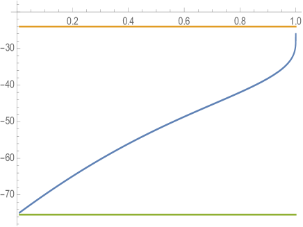
Figure 1. The function $2h(k)/W(k)$ in blue. The yellow line is at $y=-24=\lim_{k\to 1-}\frac{2h(k)}{W(k)}$, while the red line is at $y=-24\pi=\lim_{k\to 0+}\frac{2h(k)}{W(k)}$

5. Spectral stability for the periodic waves in the cubic model

Our main result for the cubic model is the following.

Theorem 3.

The waves constructed in (27) and (28) are spectrally stable with respect to co-periodic perturbations.

The proof of Theorem 3 follows path similar to the proof of Theorem 2. We first rule out complex instabilities. For the real instabilities, we need to use Theorem 1 for specific co-dimension two subspace $Z:Z\perp Ker(L)$. Finally, we need to verify that $L^{-1}|_{Z}<0$, which reduces to verifying the same type of quantity as before.

Based on the information for the operator $L$ in (35), we have the following spectral picture

$$\left\{\begin{array}[]{l}\sigma(L)=\{-\sigma_{0}^{2}\}\cup\{-\sigma_{1}^{2}\}\cup\{0\}\cup\sigma_{+}(L)\\ L\chi_{0}=-\sigma_{0}^{2}\chi_{0},L\chi_{1}=-\sigma_{1}^{2}\chi_{1}L[\Phi]=0.\end{array}\right.$$

Note that $\chi_{0},\chi_{1}$ are even functions, while $\Phi$ is an odd function. Next, we are considering the eigenvalue problem (19). Taking dot product with the constant $1$ yields

$$\langle L[Z],1\rangle=\mu\langle Z^{\prime},1\rangle=0.$$

Thus, $\langle Z,L[1]\rangle=\langle L[Z],1\rangle=0$, whence $Z\perp L[1]=\Phi^{2}-c$. Taking dot product of (19) with $\Phi$, we obtain

$$\mu\langle Z^{\prime},\Phi\rangle=\langle L[Z],\Phi\rangle=\langle Z,L[\Phi]\rangle=0,$$

whence $Z\perp\Phi^{\prime}$.

5.1. Proof of Theorem 3: Ruling out complex instabilities

We now rule out complex instabilities. We proceed in the same way as in the derivation of (46) and subsequently (47), (50), (51). Instead of verifying the quantity (52) however, we now compute

$$\langle Lu_{2},u_{2}\rangle+\langle Lv_{2},v_{2}\rangle = \mu_{1}(\langle u_{1}^{\prime},u_{2}\rangle+\langle v_{1}^{\prime},v_{2}\rangle)+\mu_{2}(\langle u_{1}^{\prime},v_{2}\rangle-\langle v_{1}^{\prime},u_{2}\rangle)=$$

$$= \mu_{1}(\langle u_{1}^{\prime},u_{2}\rangle+\langle u_{2}^{\prime},u_{1}\rangle)+\mu_{2}(\langle u_{1}^{\prime},v_{2}\rangle+\langle v_{2}^{\prime},u_{1}\rangle)=0.$$

where we have used (50) and (51). But now, $u_{2},v_{2}$ are both odd functions and as such, project on the non-negative subspace of $L$ (recall that the negative subspace is spanned by $\chi_{0},\chi_{1}$, both even functions). Thus, it follows that $\langle Lu_{2},u_{2}\rangle=0$ and $\langle Lv_{2},v_{2}\rangle=0$, whence

$$u_{2}=C_{1}\Phi,v_{2}=C_{2}\Phi.$$

Putting this back in (47) yields in particular

$$\left|\begin{array}[]{l}\mu_{1}u_{1}^{\prime}-\mu_{2}v_{1}^{\prime}=0\\ \mu_{2}u_{1}^{\prime}+\mu_{1}v_{1}^{\prime}=0\end{array}\right.$$

Since $\mu_{1}\neq 0,\mu_{2}\neq 0$, it follows that $u_{1}=A_{1},v_{1}=B_{1}$. But then again from (47), we obtain

$$\left|\begin{array}[]{l}A_{1}L[1]=(\mu_{1}C_{1}-\mu_{2}C_{2})\Phi^{\prime}\\ B_{1}L[1]=(\mu_{2}C_{1}+\mu_{1}C_{2})\Phi^{\prime}.\end{array}\right.$$

Since $L[1]=\Phi^{2}-c\neq\Phi^{\prime}$, we have $A_{1}=B_{1}=0$ and $C_{1}=C_{2}=0$, which is the zero solution for the spectral problem, a contradiction.

5.2. Proof of Theorem 3: Ruling out real instabilities

In this section, we rule out the real instabilities. Assume for a contradiction that there is $\mu>0$, so that the eigenvalue problem (19) has a solution $Z=u+v$, where $u$ is even and $v$ is an odd function. We have then

(57) $$\left|\begin{array}[]{l}Lu=\mu v^{\prime}\\ Lv=\mu u^{\prime}\end{array}\right.$$

Taking dot products with $u$ and $v$ respectively and adding

(58) $$\langle Lu,u\rangle+\langle Lv,v\rangle=\mu(\langle v^{\prime},u\rangle+\langle u^{\prime},v\rangle)=0.$$

Again, the odd function $v$ projects over the non-negative subspace of $L$ only. Thus, $\langle Lv,v\rangle\geq 0$. Assume first that $\langle Lv,v\rangle=0$. It follows that $v=c_{0}\Phi$ for some constant $c_{0}$. It follows from (57) that

$$\mu u^{\prime}=L[c_{0}\Phi]=0,$$

whence $u=c_{1}$. But then, from the other equation in (57),

$$c_{1}L[1]=\mu c_{0}\Phi^{\prime}.$$

Again $L[1]=\Phi^{2}-c\neq\Phi^{\prime}$ and this is only possible if $c_{1}=c_{0}=0$, a contradiction.

Thus, it must be that $\langle Lv,v\rangle>0$. By (58), this implies that $\langle Lu,u\rangle<0$. We will show that this leads to a contradiction as well.

We need the following simple lemma.

Lemma 2.

Let $\mathcal{X}$ be a real Hilbertian space, with $Z=span\{\eta_{1},\eta_{2}\}\subset\mathcal{X}$, where $\eta_{1},\eta_{2}:\eta_{1}\perp\eta_{2}$. Let $A$ be a self-adjoint operator on $\mathcal{X}$. Then $A|_{Z}<0$ if and only if the matrix

$$D=(D_{ij})_{i,j=1,2},\ \ D_{ij}=\langle A\eta_{i},\eta_{j}\rangle.$$

is negative definite. Equivalently, $D$ is negative definite if

$$\langle A\eta_{1},\eta_{1}\rangle<0,\det(D)>0.$$

Proof.

Assume $A|_{Z}<0$. Immediately, $\langle A\eta_{1},\eta_{1}\rangle<0$. Let

$$g(\lambda):=\langle A(\lambda\eta_{1}+\eta_{2}),\lambda\eta_{1}+\eta_{2}\rangle=\lambda^{2}\langle A\eta_{1},\eta_{1}\rangle+2\lambda\langle A\eta_{1},\eta_{2}\rangle+\langle A\eta_{2},\eta_{2}\rangle.$$

In particular, $g(\lambda)<0$ for all $\lambda$. Thus, the quadratic function $\lambda\to g(\lambda)$ does not have real roots, that is

$$\langle A\eta_{1},\eta_{2}\rangle^{2}-\langle A\eta_{1},\eta_{1}\rangle\langle A\eta_{2},\eta_{2}\rangle<0.$$

Since $\det(D)=-(|\langle A\eta_{1},\eta_{2}\rangle|^{2}-\langle A\eta_{1},\eta_{1}\rangle\langle A\eta_{2},\eta_{2}\rangle)>0$, we have shown one direction.

Conversely, assume that $D$ is negative definite. Then since $\det(D)>0$, it follows that $g(\lambda)=0$ does not have real solutions. This, paired with $\langle A\eta_{1},\eta_{1}\rangle<0$ implies that $g(\lambda)<0$ for all real $\lambda$, which in turn means that $A|_{Z}<0$. ∎

We claim that in order to obtain a contradiction, it is enough to show

(59) $$L^{-1}|_{span\{\Phi^{\prime},\Phi^{2}-c\}}<0.$$

Indeed, since we already have that $Z=u+v\perp\Phi^{\prime}$ and $v\perp\Phi^{\prime}$ (as an odd function), we conclude that $u\perp\Phi^{\prime}$. Similarly, $Z=u+v\perp\Phi^{2}-c$, $v\perp\Phi^{2}-c$ (as an odd function), whence $u\perp\Phi^{2}-c$. Overall, $u\in span\{\Phi^{\prime},\Phi^{2}-c\}^{\perp}$. On the other hand, if (59) holds, by Theorem 1, we would conclude $L|_{span\{\Phi^{\prime},\Phi^{2}-c\}^{\perp}}\geq 0$, so in particular $\langle Lu,u\rangle\geq 0$, a contradiction with (58), which implies $\langle Lu,u\rangle<0$. Thus, matters have been reduced to showing (59).

By Lemma 2, in order to prove (59), it is enough to show that the matrix

$$D=\left(\begin{array}[]{cc}\langle L^{-1}[\Phi^{\prime}],\Phi^{\prime}\rangle&\langle L^{-1}[\Phi^{2}-c],\Phi^{\prime}\rangle\\ \langle L^{-1}[\Phi^{\prime}],\Phi^{2}-c\rangle&\langle L^{-1}[\Phi^{2}-c],\Phi^{2}-c\rangle\end{array}\right)$$

is negative definite. We have (recalling $\Phi^{2}-c=L[1]$),

$$\langle L^{-1}[\Phi^{\prime}],\Phi^{2}-c\rangle=\langle\Phi^{\prime},L^{-1}[\Phi^{2}-c]\rangle=\langle\Phi^{\prime},L^{-1}[L[1]]\rangle=\langle\Phi^{\prime},1\rangle=0.$$

Also,

$$\langle L^{-1}[\Phi^{2}-c],\Phi^{2}-c\rangle=\langle L^{-1}[L[1]],\Phi^{2}-c\rangle=\langle 1,\Phi^{2}-c\rangle<0,$$

where in the last step, we have made use of (29). Thus, the matrix $D$ is diagonal, with $D_{22}<0$. It would follow that $D$ is negative definite, if we can verify that $D_{11}<0$. Thus, we have reduced matters, again, to showing that

(60) $$\langle L^{-1}[\Phi^{\prime}],\Phi^{\prime}\rangle<0.$$

5.3. Computing $\langle L^{-1}[\Phi^{\prime}],\Phi^{\prime}\rangle$

By rescaling and from (35), we may take $L$ as follows

$$L = -\partial_{y}^{2}+2\kappa^{2}sn^{2}(y,k)-(1+\kappa^{2})$$

$$\Phi = sn(y,k),-2K(\kappa)\leq y\leq 2K(\kappa).$$

As before, the first order of business is to construct the Green’s function. We need a second function in the kernel of $L$, in addition of $\Phi$. Normally, we would take $\Psi(x)=\Phi(x)\int^{x}\frac{1}{\Phi^{2}(y)}dy,$ but note that the (definite) integral would be divergent over any interval containing zero, because of the quadratic singularity of $sn(y,k)$ at $y=0$. Instead, one integrates by parts and we come up with an equivalent expression, which is however well-defined. Namely, using that

$$\frac{1}{sn^{2}(x,\kappa)}=-\frac{1}{dn(x,\kappa)}\frac{\partial}{\partial x}\frac{cn(x,\kappa)}{sn(x,\kappa)}$$

and (formally) integrating by parts, we get

(61) $$\Psi(x)=-\frac{cn(x,\kappa)}{dn(x,\kappa)}+\kappa^{2}sn(x,\kappa)\int_{0}^{x}{\frac{cn^{2}(y,\kappa)}{dn^{2}(y,\kappa)}}dy.$$

This formula makes sense - note the lack of singularity in the denominator. Interestingly, for fixed $\kappa$, the function $x\to\Psi(x,\kappa)$ turns out to be a periodic function in the basis interval $[-2K(\kappa),2K(\kappa)]$, but its derivative $x\to\partial_{x}\Psi(x,\kappa)$ is not periodic anymore at $\pm 2K(\kappa)$.

Define the Wronskian by the standard formula

$$W[\kappa]=\Psi^{\prime}(x,\kappa)\Phi(x,\kappa)-\Psi(x,\kappa)\Phi^{\prime}(x,\kappa).$$

Using Mathematica, we have found that $W[\kappa]=1$, which confirms once again that the function $\Psi$ constructed in (61) is another non-trivial solution of $L\Psi=0$. We can now represent for any $f\in L^{2}_{per}[-2K(\kappa),2K(\kappa)]$,

$$L^{-1}f(x)=\frac{1}{2}\left(\Phi(x)\int_{-2K(\kappa)}^{x}\Psi(y)f(y)dy-\Psi(x)\int_{-2K(\kappa)}^{x}\Phi(y)f(y)dy\right)+C_{f}\Psi(x).$$

where the constant $C_{f}$ is to be selected so that the function $x\to L^{-1}f(x)$ is periodic in $[-2K(\kappa),2K(\kappa)]$.

For the function of interest, namely $f=\Phi^{\prime}$, we find that $L^{-1}f(-2K(k))=L^{-1}f(2K(\kappa))$ for all values of $C$, but when we impose the condition $\partial_{x}L^{-1}f|_{x=-2K(k)}=\partial_{x}L^{-1}f|_{x=2K(k)}$, we come up with a condition for $C_{\Phi^{\prime}}$

$$C_{\Phi^{\prime}}=\frac{1}{4\Psi^{\prime}(2K(\kappa))}\int_{-2K(\kappa)}^{2K(\kappa)}\Psi(x)\Phi^{\prime}(x)dx.$$

Now that we have a proper formula for $L^{-1}[\Phi^{\prime}]$, we may compute

$$\langle L^{-1}[\Phi^{\prime}],\Phi^{\prime}\rangle = \frac{1}{2}\left[\left\langle\Phi\int_{-2K(\kappa)}^{x}{\Psi(y)\Phi^{\prime}(y)}dy,\Phi^{\prime}\right\rangle-\left\langle\Psi(x)\int_{-2K(\kappa)}^{x}{\Phi(y)\Phi^{\prime}(y)}dy,\Phi^{\prime}\right\rangle\right]+$$

$$+ \frac{1}{4\Psi^{\prime}(2K(\kappa))}(\langle\Psi,\Phi^{\prime}\rangle)^{2}.$$

After integrating by parts, we get

$$\left\langle\Phi\int_{-2K(\kappa)}^{x}{\Psi(y)\Phi^{\prime}(y)}dy,\Phi^{\prime}\right\rangle=-\frac{1}{2}\int_{-2K(\kappa)}^{2K(\kappa)}{\Phi^{2}(x)\Phi^{\prime}(x)\Psi(x)}dx$$

and

$$\left\langle\Psi(x)\int_{-2K(\kappa)}^{x}{\Phi(y)\Phi^{\prime}(y)}dy,\Phi^{\prime}\right\rangle=\frac{1}{2}\int_{-2K(\kappa)}^{2K(\kappa)}{\Phi^{2}\Phi^{\prime}\Psi}dx.$$

Putting it together in the formula for $\langle L^{-1}[\Phi^{\prime}],\Phi^{\prime}\rangle$, we obtain

(62) $$\langle L^{-1}[\Phi^{\prime}],\Phi^{\prime}\rangle=-\frac{1}{2}\int_{-2K(\kappa)}^{2K(\kappa)}{\Phi^{2}\Phi^{\prime}\Psi}dx+\frac{1}{4\Psi^{\prime}(2K(\kappa))}\left(\int_{-2K(\kappa)}^{2K(\kappa)}\Psi\Phi^{\prime}\right)^{2}.$$

Clearly, this last expression is a function of $\kappa$ only. Computing precisely the integrals by hand is not easy, even though some of them result in simple expressions, for example

$$\int_{-2K(\kappa)}^{2K(\kappa)}\Psi\Phi^{\prime}=-2K(\kappa).$$

We use Mathematica for the symbolic integration to obtain the precise formulas. Below, we provide the graph of the resulting function, from which it is clear that (60) is satisfied.

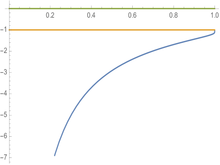
Figure 2. The function $\kappa\to\langle L^{-1}[\Phi^{\prime}],\Phi^{\prime}\rangle$ in blue. The orange line is $y=-1=\lim_{k\to 1-}\langle L^{-1}[\Phi^{\prime}],\Phi^{\prime}\rangle$.

6. The parabolic peakons are “unstable” in the absence of periodic boundary conditions

As we have discussed in the previous sections, the parabolic peakons may be considered as limit solutions of the arise as a limit of the stable snoidal solutions of the Ostrovsky model introduced in (23). In that sense, one might be tempted to claim that they are stable. We have however left this question open. This is partially due to the difficulty of defining an appropriate boundary conditions for the corresponding linearized problem. In this section, we construct (almost explicitly) solutions of (18), which lack the required periodic properties, but are nevertheless smooth inside $(-L,L)$ and satisfy the equation in classical sense. So, one can say that in a way the parabolic peakons are unstable, once the perturbations are allowed to have “wild” boundary conditions.

Theorem 4.

The parabolic peakons $\varphi$, given by (41) are spectrally unstable for all $L>0$ in the sense that there exists $z\in C^{2}(-L,L)$ (in fact $z\in C^{\infty}(-L,L)$) so that (12) is satisfied in a classical sense for $\xi\in(-L,L)$.

Note: As we establish below, the $2L$ periodization of the function $z$ constructed here is not even continuous at $\pm L$, since

$$\lim_{\xi\to-L+}z(\xi)\neq 0,\ \ \lim_{\xi\to L-}z(\xi)=0.$$

Thus, the instability result claimed in Theorem 4 is not in the sense of Definition 1, but rather in a milder sense, see the precise description above.

Proof.

Our proof proceeds via the same approach, via the change of variables (7). In this simple case, with the explicit formula (41), we will be able however to explicitly calculate $\xi=\xi(\eta)$ and its inverse. Indeed, taking derivative in $\eta$ in (7), we obtain

(63) $$\frac{d\Xi}{d\eta}=1-\frac{\Psi^{\prime}(\eta)}{c}=1-\frac{\varphi(\xi)}{c}=\frac{3}{2L^{2}}(L^{2}-\xi^{2}).$$

Treating this last equality as a separable ODE, we have $\frac{d\xi}{L^{2}-\xi^{2}}=\frac{3}{2L^{2}}d\eta$. By integrating the ODE, we obtain the formula

$$\xi=L\frac{Ce^{\frac{e^{3\eta}}{L}}-1}{Ce^{\frac{e^{3\eta}}{L}}+1}.$$

This gives us an arbitrary solution of (63). We set $C=1$ as a particular solution, which gives us

(64) $$\xi=\Xi(\eta)=L\frac{e^{\frac{e^{3\eta}}{L}}-1}{e^{\frac{e^{3\eta}}{L}}+1}=L\tanh(3\eta/(2L)).$$

Clearly, the function $\Xi:(-\infty,\infty)\to(-L,L)$ is one-to-one and it has an inverse function $\eta=\eta(\xi):(-L,L)\to(-\infty,\infty)$. Thus, in this case the interval $(-M,M)$, which we used to get from inverting the transformation $\xi=\Xi(\eta)$ is actually degenerate, in that $M=\infty$. Using this last formula in (41), we obtain a formula for $\Phi$. More precisely,

(65) $$\Phi(\eta)=\varphi(\Xi(\eta))=\frac{L^{2}}{6}\tanh^{2}(3\eta/(2L))-\frac{L^{2}}{18}=\frac{L^{2}}{9}\left(1-\frac{3}{2}\operatorname{sech}^{2}(3\eta/(2L))\right).$$

Note that $-c+\Phi=-\frac{L^{2}}{6}\operatorname{sech}^{2}(3\eta/(2L))$. We will show that for some $\mu>0$, the resulting eigenvalue problem

(66) $$(-\frac{L^{2}}{81}\partial_{\eta\eta}-\frac{1}{6}\operatorname{sech}^{2}(3\eta/(2L)))Z=\pm\mu Z_{\eta},\ \ -\infty<\eta<\infty,$$

has a solution $Z$.

We make a few more transformation for (66). If we take $f:Z(\eta)=f(3\eta/(2L)),$ it leads us into the equivalent eigenvalue problem

(67) $$-f^{\prime\prime}(x)-6\operatorname{sech}^{2}(x)f(x)=\pm\mu_{1}f^{\prime}(x),\ \ x\in\mathbf{R}^{1},$$

where $\mu_{1}=\frac{54\mu}{L}$.

Next, we change variables to reduce (67) to a regular static Schrödinger equation, i.e. one where is no first derivative terms. To this end, fix the plus sign in (67). Take $q:f(x)=e^{-\frac{\mu_{1}}{2}x}q(x)$. Plugging this into (67) results in the new equation in terms of $q$

(68) $$-q^{\prime\prime}(x)-6\operatorname{sech}^{2}(x)q(x)=-\frac{\mu_{1}^{2}}{4}q(x).$$

In this form, we can solve the problem explicitly. Indeed,

$$\mathcal{L}=-\partial_{x}^{2}-6\operatorname{sech}^{2}(x)=L_{+}-1$$

where $L_{+}$ is the Schrödinger operator arising in the linearization around the soliton $sech(x)$ in the cubic NLS. As such, we know that for $q_{1}:=-\operatorname{sech}^{\prime}(x)=\operatorname{sech}(x)\tanh(x)$, $L_{+}[q_{1}]=0$ or in terms of $\mathcal{L}$, for $\mu_{1}=2$, we have

(69) $$-q_{1}^{\prime\prime}-6\operatorname{sech}^{2}(x)q_{1}=-q_{1}.$$

From this last formula for $q_{1}$, it is clear that the ($2L$ periodization of the) corresponding function $z$ cannot be even continuous at $\pm L$. Indeed,

$$\lim_{\xi\to-L+}z(\xi)=\lim_{\eta\to-\infty}Z(\eta)=\lim_{x\to-\infty}f(x)=\lim_{x\to-\infty}e^{-x}\operatorname{sech}(x)\tanh(x)=-2$$

On the other hand

$$\lim_{\xi\to L-}z(\xi)=\lim_{x\to\infty}e^{-x}f(x)=0.$$

Hence, we establish that the $2L$ periodization of the function $z$ constructed here is not even continuous at $\pm L$. On the other hand, $z\in C^{\infty}(-L,L)$ and it satisfies the eigenvalue equation (12) for $\xi\in(-L,L)$ by tracing back the changes of variables.

∎

References

- [1] J. P. Boyd, Ostrovsky and Hunter A generic wave equation for weakly dispersive waves: Matched asymptotic and pseudo-spectral study of the paraboloidal travelling waves (corner and near-corner waves), Euro. J. Appl. Maths. 16,(2004), p. 65–81.
- [2] N. Costanzino, V. Manukian, C,K.R.T. Jones, Solitary waves of the regularized short pulse and Ostrovsky equations SIAM J. Math. Anal. 41 (2009), no. 5, p. 2088–2106.
- [3] N. Costanzino, V. Manukian, C,K.R.T. Jones, B. Sandstede, Existence of multi-pulses of the regularized short-pulse and Ostrovsky equations. J. Dynam. Differential Equations 21 (2009), no. 4, p. 607–622.
- [4] T. Gallay, D. Pelinovsky, Orbital stability in the cubic defocusing NLS equation. Part I: Cnoidal periodic waves J. Diff. Eqs. 258 (2015), p. 3607–3638.
- [5] R. Grimshaw, L. A. Ostrovsky, V. I. Shrira, Y. Stepanyants Long nonlinear surface and internal gravity waves in a rotating ocean, Surv. Geophys. 19, (1998), p. 289–338
- [6] R. Grimshaw, K. Helfrich, E.R. Johnson, The reduced Ostrovsky equation: integrability and breaking. Stud. Appl. Math. 129, (2012), no. 4, p. 414–436.
- [7] R. Grimshaw, D. Pelinovsky, Global existence of small-norm solutions in the reduced Ostrovsky equation. Discrete Contin. Dyn. Syst. 34 (2014), no. 2, 557–566.
- [8] S. Hakkaev, M. Stanislavova, A. Stefanov, Periodic traveling waves of the short pulse equation: existence and stability, submitted.
- [9] S. Hakkaev, I.D. Iliev, K. Kirchev, Stability of periodic travelling shallow-water waves determined by Newton’s equation. J. Phys. A: Math. Theor. 41 (2008), 31 pp.
- [10] E. Johnson, D. Pelinovsky, Orbital stability of periodic waves in the class of reduced Ostrovsky equations, available at arXiv:1603.02961.
- [11] J. K. Hunter, Numerical solution of some nonlinear dispersive wave equations, in Computational Solution of Nonlinear Systems of Equations, Vol. 26 (E. L. Allgower and K. Georg, Eds.),1990), pp. 301– 316, Lectures in Applied Mathematics.
- [12] S. Levandosky, Y. Liu, Stability of solitary waves of a generalized Ostrovsky equation. SIAM J. Math. Anal. 38 (2006), no. 3, p. 985–1011.
- [13] S. Levandosky, Y. Liu, Stability and weak rotation limit of solitary waves of the Ostrovsky equation. Discrete Contin. Dyn. Syst. Ser. B 7 (2007), no. 4, p. 793–806.
- [14] Y. Liu, On the stability of solitary waves for the Ostrovsky equation. Quart. Appl. Math. 65 (2007), no. 3, p. 571–589.
- [15] Y. Liu, M. Ohta, Stability of solitary waves for the Ostrovsky equation. Proc. Amer. Math. Soc. 136 (2008), no. 2, p. 511–517.
- [16] Y. Liu, D. Pelinovsky, A. Sakovich, Wave breaking in the short-pulse equation. Dyn. Partial Differ. Equ. 6 (2009), no. 4, p. 291–310.
- [17] Y. Liu, D. Pelinovsky, A. Sakovich, Wave breaking in the Ostrovsky-Hunter equation. , SIAM J. Math. Anal. 42 (2010), no. 5, p. 1967–1985.
- [18] A.J. Morrisson, E.J. Parkes and V.O. Vakhnenko, The N loop soliton solutions of the Vakhnenko equation, Nonlinearity 12, 1427-1437 (1999).
- [19] L. A. Ostrovsky, Nonlinear internal waves a in rotating ocean, Oceanology, 18 (1978), p. 119–125.
- [20] A. Sakovich and S. Sakovich, Solitary wave solutions of the short pulse equation, J. Phys. A: Math. Gen. 39, L361-L367 (2006).
- [21] T. Schäfer, C.E. Wayne, Propagation of ultra-short optical pulses in cubic nonlinear media. Physica D 196 (2004), no. 1-2, 90–105.
- [22] A. Stefanov, Y. Shen, P. Kevrekidis, Well-posedness and small data scattering for the generalized Ostrovsky equation. J. Differential Equations 249 (2010), no. 10, p. 2600–2617.
- [23] Y. A. Stepanyants, On stationary solutions of the reduced Ostrovsky equation: Periodic waves, compactons and compound solitons, Chaos, Solitons Fract. 28 (2006) p. 193–204.
- [24] V A. Vakhnenko, Solitons in a nonlinear model medium, J. Phys. A: Math. Gen. 25 , (1992), p. 4181–4187.
- [25] V.O. Vakhnenko and E.J. Parkes, The two loop soliton solution of the Vakhnenko equation. Nonlinearity 11 (1998), no. 6, p. 1457–1464.
- [26] V.O. Vakhnenko and E.J. Parkes, The calculation of multi-soliton solutions of the Vakhnenko equation by the inverse scattering method, Chaos, Solitons and Fractals 13, 1819-1826 (2002).