Keplerian integrals, elimination theory and identification of very short arcs in a large database of optical observations

Abstract

The modern optical telescopes produce a huge number of asteroid observations, that are grouped into very short arcs (VSAs), each containing a few observations of the same object in one single night. To decide whether two VSAs, collected in different nights, refer to the same observed object we can attempt to compute an orbit with the observations of both arcs: this is called the linkage problem. Since the number of orbit computations to be performed is very large, we need efficient methods of orbit determination. Using the first integrals of Kepler’s motion we can write algebraic equations for the linkage problem, which can be put in polynomial form, see [3], [4], [5]. The equations introduced in [5] can be reduced to a univariate polynomial of degree 9: the unknown is the topocentric distance $\rho$ of the observed body at the mean epoch of one of the VSAs. Using elimination theory we show an optimal property of this polynomial: it has the least degree among the univariate polynomials in the same variable that are consequence of the algebraic conservation laws and are obtained without squaring operations, that can be used to bring these algebraic equations in polynomial form. In this paper we also introduce a procedure to join three VSAs belonging to different nights: from the conservation of angular momentum at the three mean epochs of the VSAs, we obtain a univariate polynomial equation of degree 8 in the topocentric distance $\rho_{2}$ at the intermediate epoch. This algorithm has the same computational complexity as the classical method by Gauss, but uses more information, therefore we expect that it can produce more accurate results. These results can be used as better preliminary orbits to compute a least squares orbital solution with three VSAs. For both methods, linking two and three VSAs, we also discuss how to select the solutions, making use of the full two-body dynamics, and show some numerical tests comparing the results with the ones obtained by Gauss’ method.

1 Introduction

We consider very short arcs (VSAs) of optical observations of a solar system body whose motion is dominated by the gravitational attraction of the Sun. These small sets of observations are called tracklets and the corresponding arc described in the sky is usually too short to compute a least squares orbit. In each observing night we can detect thousands of these data, so that it is difficult to decide whether two such arcs, collected in different nights, refer to the same observed body. This gives rise to an identification problem, that can be solved by computing an orbit with the information contained in two or more tracklets.

Using the classical methods of initial orbit determination, those by Laplace [6] or Gauss [2], we usually cannot compute a preliminary orbit with three observations belonging to the same VSA because they are too close in time and the arc is usually too short. Even using observations taken from two different VSAs it may be difficult to compute an orbit. Laplace’s or Gauss’ methods in most cases work well if we use three different observations from three VSAs. In this case to compute a preliminary orbit we have to find the roots of a univariate polynomial of degree 8 (see [9]), that correspond to the possible values of the radial distance (geocentric for Laplace, topocentric for Gauss) of the observed body at a given epoch (the mean epoch of the observations $\sum_{h=1}^{3}t_{h}/3$ for Laplace, the central epoch $t_{2}$ for Gauss).

Assume for simplicity that we deal with this identification problem using the observations made by a single telescope performing an asteroid survey, like Pan-STARRS [10], or the next generation telescope LSST [7]. The average number of observations per night is $N\approx 10^{4}$ for Pan-STARRS, and presumably we shall have $N\approx 10^{5}$ for LSST. To perform systematically the identification by Gauss’ method using the data of three observing nights we should test compatibility for $O(N^{3})$ triples of observations. This is clearly a cumbersome task. The identification of two VSAs is usually called the linkage problem, and it has been recently studied in [3], [4], [5] using the first integrals of the two-body motion.

In [5] the authors introduced a univariate polynomial equation of degree 9 for the linkage problem, which is comparable with the equation of Gauss’ method. This equation is derived in a concise way in Section 3. Moreover, we discuss an optimal property of such polynomial. Using algebraic elimination theory, we show that it has the least degree among the univariate polynomials that are consequence of the algebraic conservation laws of Kepler’s problem, provided we drop the dependence between the inverse of the heliocentric distance $1/|{\bf r}|$ appearing in the Keplerian potential and the topocentric distance $\rho$. This approach avoids the squaring operations needed in [3], [4] to bring the selected equations into a polynomial form. In Section 3.4 we sketch a method to check the validity of the identification and select solutions according to some compatibility conditions, similar to the ones in [3], that use the full two-body dynamics.

An orbit computed with two VSAs is usually not as reliable as one computed with three observations, each picked up in a different VSAs, because the latter usually represents a longer arc. To obtain more reliable results we have to join together at least three VSAs. In Section 4 we introduce a univariate polynomial equation of degree 8 to link three VSAs of optical observations by means of the conservation of angular momentum only. Then the other laws of Kepler’s motion can be used to set up restrictive compatibility conditions, allowing us to test the identification and select solutions.

Assume we set up an identification procedure with a large database of asteroid observations. For simplicity, we can consider three observing nights, in which we collect $O(N)$ VSAs of observations per night. We can try to identify pairs of VSAs belonging to the first two nights by applying $O(N^{2})$ times the linkage algorithm introduced in [5] and reviewed in Section 3. The output is composed by preliminary orbits obtained with pairs of VSAs. If the thresholds in the controls for acceptance (see Section 3.4) are well selected, we do not obtain more than $O(N)$ pairs of VSAs, in fact the number of different objects observed in the two nights is $O(N)$. Then we can apply the method to link three VSAs introduced in Section 4 to the $O(N)$ selected pairs and the $O(N)$ VSAs of the third observing night. We conclude that this identification problem can be faced by $O(N^{2})$ computations of roots of a polynomial of degree 9 or 8, instead of $O(N^{3})$ computations of roots of Gauss’ polynomial.

2 Keplerian integrals

We consider the Keplerian motion of a celestial body around a center of force, set at the origin of a given reference system, that in the asteroid case corresponds to the center of the Sun. Optical observations of the body are made by a telescope whose heliocentric position is a known function of time. Then the heliocentric position and velocity of the body are given by

$${\bf r}=\rho{\bf e}^{\rho}+{\bf q},\hskip 42.67912pt\dot{\bf r}=\dot{\rho}{\bf e}^{\rho}+\rho\bm{\eta}+\dot{\bf q},$$ (1)

where ${\bf q},\dot{\bf q}$ are the heliocentric position and velocity of the observer, $\rho,\dot{\rho}$ are the topocentric radial distance and velocity, ${\bf e}^{\rho}$ is the line of sight unit vector, which can be written in terms of the topocentric right ascension $\alpha$ and declination $\delta$ as

$${\bf e}^{\rho}=(\cos\delta\cos\alpha,\cos\delta\sin\alpha,\sin\delta).$$

Moreover in (1) we set

$$\bm{\eta}=\dot{\alpha}\cos\delta{\bf e}^{\alpha}+\dot{\delta}{\bf e}^{\delta},$$

where

$${\bf e}^{\alpha}=(\cos\delta)^{-1}\frac{\partial{\bf e}^{\rho}}{\partial\alpha},\hskip 28.45274pt{\bf e}^{\delta}=\frac{\partial{\bf e}^{\rho}}{\partial\delta},$$

and $\dot{\alpha},\dot{\delta}$ are the angular rates. The Keplerian integrals, represented by the angular momentum vector ${\bf c}$, the Laplace-Lenz vector $\mathbf{L}$ and the energy $\mathcal{E}$, are defined by

$${\bf c}={\bf r}\times\dot{\bf r},\qquad\mu{\bf L}=\Bigl{(}|\dot{\bf r}|^{2}-\frac{\mu}{|{\bf r}|}\Bigr{)}{\bf r}-({\bf r}\cdot\dot{\bf r})\dot{\bf r},\qquad{\cal E}=\frac{1}{2}|\dot{\bf r}|^{2}-\frac{\mu}{|{\bf r}|},$$ (2)

as functions of $\mathbf{r},\dot{\mathbf{r}}$. Given the values of $\alpha,\delta,\dot{\alpha},\dot{\delta}$, they can be written as algebraic functions of $\rho,\dot{\rho}$ using relations (1).

3 Linking two VSAs

Given a very short arc of optical observations ($\alpha_{i}$, $\delta_{i}$), $i=1\ldots m$, made by the same station at $t_{i}$ different times, it is often possible to compute the attributable vector (see [11])

$${\cal A}=(\alpha,\delta,\dot{\alpha},\dot{\delta})$$

at the mean epoch $\bar{t}=\frac{1}{m}\sum_{i=1}^{m}t_{i}$. The missing quantities to obtain a preliminary orbit are the topocentric distance and velocity $\rho$, $\dot{\rho}$ at $t=\bar{t}$. When the second derivatives ($\ddot{\alpha}$, $\ddot{\delta}$) are either not available (if $m=2$), or not accurate enough due to the errors in the observations, then the attributable summarizes essentially all the information contained in the VSA. In this case a preliminary orbit can be obtained by linking together two different VSAs.

The key idea of the linkage method is to use the conservation of the Keplerian integrals ${\bf c}$, ${\bf L}$, ${\cal E}$ at the two mean epochs $\bar{t}_{1},\bar{t}_{2}$ of two attributables ${\cal A}_{1},{\cal A}_{2}$:

$${\bf c}_{1}={\bf c}_{2},\qquad{\bf L}_{1}={\bf L}_{2},\qquad{\cal E}_{1}={\cal E}_{2},$$ (3)

where the indexes $1,2$ refer to the epoch.

Below we derive in a concise way the polynomial equations for the linkage problem introduced in [5], and we review the procedure to obtain the univariate polynomial of degree 9 giving the possible values for the topocentric distance $\rho_{2}$. Moreover, we show here an optimal property of this polynomial.

3.1 Conservation of angular momentum

The angular momentum as function of $\rho,\dot{\rho}$ can be written as

$${\bf c}(\rho,\dot{\rho})={\bf r}\times\dot{\bf r}={\bf D}\dot{\rho}+{\bf E}\rho^{2}+{\bf F}\rho+{\bf G},$$

where

$$\begin{array}[]{l}{\bf D}={\bf q}\times{\bf e}^{\rho},\cr{\bf E}=\dot{\alpha}\cos\delta{\bf e}^{\rho}\times{\bf e}^{\alpha}+\dot{\delta}{\bf e}^{\rho}\times{\bf e}^{\delta}=\dot{\alpha}\cos\delta{\bf e}^{\delta}-\dot{\delta}{\bf e}^{\alpha},\cr{\bf F}=\dot{\alpha}\cos\delta{\bf q}\times{\bf e}^{\alpha}+\dot{\delta}{\bf q}\times{\bf e}^{\delta}+{\bf e}^{\rho}\times\dot{\bf q},\cr{\bf G}={\bf q}\times\dot{\bf q}.\cr\end{array}$$

Then the equation

$${\bf c}_{1}={\bf c}_{2},$$

representing the conservation of the angular momentum are written as

$${\bf D}_{1}\dot{\rho}_{1}-{\bf D}_{2}\dot{\rho}_{2}={\bf J}(\rho_{1},\rho_{2}),$$ (4)

where

$${\bf J}(\rho_{1},\rho_{2})={\bf E}_{2}\rho_{2}^{2}-{\bf E}_{1}\rho_{1}^{2}+{\bf F}_{2}\rho_{2}-{\bf F}_{1}\rho_{1}+{\bf G}_{2}-{\bf G}_{1}.$$ (5)

We can eliminate the radial velocities $\dot{\rho}_{1},\dot{\rho}_{2}$ by making the scalar product with ${\bf D}_{1}\times{\bf D}_{2}$, that gives the quadratic polynomial

$$q(\rho_{1},\rho_{2}):={\bf D}_{1}\times{\bf D}_{2}\cdot{\bf J}(\rho_{1},\rho_{2})=0$$ (6)

in the variables $\rho_{1},\rho_{2}$. The radial velocities are given by

$$\small\dot{\rho}_{1}(\rho_{1},\rho_{2})=\frac{({\bf J}\times{\bf D}_{2})\cdot({\bf D}_{1}\times{\bf D}_{2})}{|{\bf D}_{1}\times{\bf D}_{2}|^{2}},\hskip 11.38092pt\dot{\rho}_{2}(\rho_{1},\rho_{2})=\frac{({\bf J}\times{\bf D}_{1})\cdot({\bf D}_{1}\times{\bf D}_{2})}{|{\bf D}_{1}\times{\bf D}_{2}|^{2}}.$$ (7)

These expressions are obtained by projecting (4) onto the vectors ${\bf D}_{1}\times({\bf D}_{1}\times{\bf D}_{2})$ and ${\bf D}_{2}\times({\bf D}_{1}\times{\bf D}_{2})$, generating the plane orthogonal to ${\bf D}_{1}\times{\bf D}_{2}$. Therefore using such expressions of $\dot{\rho}_{1},\dot{\rho}_{2}$ we have

$$({\bf c}_{1}-{\bf c}_{2})\times({\bf D}_{1}\times{\bf D}_{2})={\bf 0}$$

whatever the values of $\rho_{1},\rho_{2}$.

3.2 The univariate polynomial $\mathfrak{u}$

By relations (7) we can eliminate the dependence on $\dot{\rho}_{1},\dot{\rho}_{2}$ in the Laplace-Lenz and energy conservation laws

$${\bf L}_{1}={\bf L}_{2},\hskip 28.45274pt{\cal E}_{1}={\cal E}_{2}.$$ (8)

These are algebraic equations in $\rho_{1},\rho_{2}$ that are not polynomial because of the terms $1/|{\bf r}_{1}|,1/|{\bf r}_{2}|$. However, in the equation

$$\bm{\xi}:=\bigl{[}\mu({\bf L}_{1}-{\bf L}_{2})-({\cal E}_{1}{\bf r}_{1}-{\cal E}_{2}{\bf r}_{2})\bigr{]}\times({\bf r}_{1}-{\bf r}_{2})={\bf 0},$$ (9)

which is a consequence of (8), the terms $1/|{\bf r}_{1}|,1/|{\bf r}_{2}|$ cancel out. The monomials of $\bm{\xi}$ with the highest total degree, i.e. 6, are all parallel to ${\bf e}^{\rho}_{1}\times{\bf e}^{\rho}_{2}$, so that we consider the bivariate polynomials

$$p_{1}=\bm{\xi}\cdot{\bf e}^{\rho}_{1},\qquad p_{2}=\bm{\xi}\cdot{\bf e}^{\rho}_{2}$$ (10)

having total degree 5. In [5] the authors show that the overdetermined bivariate polynomial system

$$q=0,\qquad\bm{\xi}={\bf 0}$$

is consistent, i.e. its set of solutions in $\mathbb{C}^{2}$ is not empty, and is equivalent to

$$q=p_{1}=p_{2}=0.$$

Moreover, if we consider the resultants (see [1])

$$\mathfrak{u}_{1}=\mathrm{Res}(p_{1},q,\rho_{1}),\hskip 28.45274pt\mathfrak{u}_{2}=\mathrm{Res}(p_{2},q,\rho_{1}),$$

then the greatest common divisor of $\mathfrak{u}_{1}$ and $\mathfrak{u}_{2}$,

$$\mathfrak{u}=\mathrm{gcd}(\mathfrak{u}_{1},\mathfrak{u}_{2}),$$ (11)

is a univariate polynomial in the variable $\rho_{2}$ of degree 9.

Remark 1

Since in this problem the role of $\rho_{1}$ and $\rho_{2}$ is symmetric, for a generic choice of the data ${\cal A}_{j},{\bf q}_{j},\dot{\bf q}_{j},j=1,2$, we obtain an analogous result by eliminating the variable $\rho_{2}$, instead of $\rho_{1}$, from $p_{1},p_{2}$.

We also recall the construction used in [5] to compute $\mathfrak{u}_{j}$, $j=1,2$. We can write

$$q(\rho_{1},\rho_{2})=\sum_{h=0}^{2}b_{h}(\rho_{2})\rho_{1}^{h},$$

where

$$b_{0}(\rho_{2})=q_{0,2}\rho_{2}^{2}+q_{0,1}\rho_{2}+q_{0,0},\qquad b_{1}=q_{1,0},\qquad b_{2}=q_{2,0},$$

with the coefficients $q_{h,k}$ depending only on the data ${\cal A}_{j},{\bf q}_{j},\dot{\bf q}_{j}$, $j=1,2$. Moreover, we have

$$p_{1}(\rho_{1},\rho_{2})=\sum_{h=0}^{4}a_{1,h}(\rho_{2})\rho_{1}^{h},\hskip 28.45274ptp_{2}(\rho_{1},\rho_{2})=\sum_{h=0}^{5}a_{2,h}(\rho_{2})\rho_{1}^{h},$$ (12)

for some univariate polynomials $a_{k,h}$ whose degrees are described by the upper small circles used to construct Newton’s polygons of $p_{1},p_{2}$ in Figure 1.

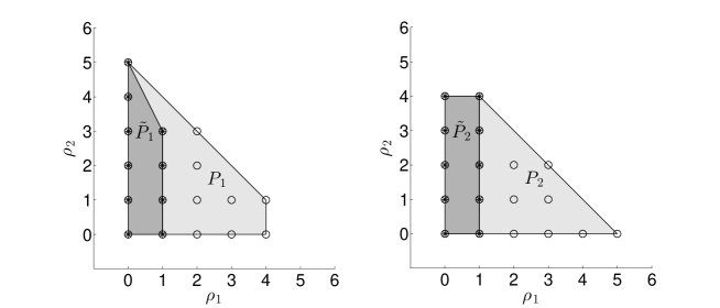
Figure 1: We draw Newton’s polygons $P_{j}$, $\tilde{P}_{j}$ for the polynomials $p_{j},\tilde{p}_{j}$, $j=1,2$. In this figure the polygons are overlapping: the nodes with circles correspond to the (multi-index) exponents of the monomials in $p_{j}$; the nodes with asterisks correspond to the exponents of the monomials in $\tilde{p}_{j}$.

Assume $q_{2,0},q_{0,2}\neq 0$. From $q=0$ we obtain

$$\rho_{1}^{h}=\beta_{h}\rho_{1}+\gamma_{h},\qquad h=2,3,4,5,$$ (13)

where

$$\beta_{2}=-\frac{b_{1}}{b_{2}},\qquad\gamma_{2}=-\frac{b_{0}}{b_{2}},$$

and

$$\beta_{h+1}=\beta_{h}\beta_{2}+\gamma_{h},\qquad\gamma_{h+1}=\beta_{h}\gamma_{2},\qquad h=2,3,4.$$

Inserting (13) into (12) we obtain

$$\tilde{p}_{j}(\rho_{1},\rho_{2})=\tilde{a}_{j,1}(\rho_{2})\rho_{1}+\tilde{a}_{j,0}(\rho_{2}),\hskip 28.45274ptj=1,2,$$ (14)

where

$$\tilde{a}_{1,1}=a_{1,1}+\sum_{h=2}^{4}a_{1,h}\beta_{h},\hskip 14.22636pt\tilde{a}_{1,0}=a_{1,0}+\sum_{h=2}^{4}a_{1,h}\gamma_{h},$$ (15)

$$\tilde{a}_{2,1}=a_{2,1}+\sum_{h=2}^{5}a_{2,h}\beta_{h},\hskip 14.22636pt\tilde{a}_{2,0}=a_{2,0}+\sum_{h=2}^{5}a_{2,h}\gamma_{h}.$$ (16)

In Figure 1 we also draw Newton’s polygons of $\tilde{p}_{1}$, $\tilde{p}_{2}$. In this case the nodes with asterisks correspond to the exponents of the monomials in $\tilde{p}_{j}$ and the upper asterisks describe the degrees of the polynomials $\tilde{a}_{k,h}$.

Let us introduce the polynomials

$$\mathfrak{v}_{1}=\mathrm{Res}(\tilde{p}_{1},q,\rho_{1}),\hskip 28.45274pt\mathfrak{v}_{2}=\mathrm{Res}(\tilde{p}_{2},q,\rho_{1}).$$

We can show the following result.

Lemma 1

By the properties of resultants we find that

$$\mathfrak{u}_{1}=q_{2,0}^{3}\mathfrak{v}_{1},\qquad\mathfrak{u}_{2}=q_{2,0}^{4}\mathfrak{v}_{2}.$$ (17)

Proof. We prove the first relation; the proof of the second one is similar. We have

$$\mathfrak{u}_{1}=\mathrm{Res}(p_{1},q,\rho_{1})=\det\left[\begin{array}[]{cccccc}a_{10}&0&b_{0}&0&0&0\\ a_{11}&a_{10}&b_{1}&b_{0}&0&0\\ a_{12}&a_{11}&b_{2}&b_{1}&b_{0}&0\\ a_{13}&a_{12}&0&b_{2}&b_{1}&b_{0}\\ a_{14}&a_{13}&0&0&b_{2}&b_{1}\\ 0&a_{14}&0&0&0&b_{2}\end{array}\right].$$

By performing raw operations and by the properties of determinants we obtain

$$\mathrm{Res}(p_{1},q,\rho_{1}) = \det\left[\begin{array}[]{cccccc}a_{10}&0&b_{0}&0&0&0\\ a_{11}+\gamma_{2}a_{13}+\beta_{2}\gamma_{2}a_{14}&\tilde{a}_{10}&b_{1}&0&0&0\\ a_{12}+\beta_{2}a_{13}+(\beta_{2}^{2}+\gamma_{2})a_{14}\hskip 2.84544pt&\tilde{a}_{11}&b_{2}&0&0&0\\ a_{13}+\beta_{2}a_{14}&a_{12}+\beta_{2}a_{13}+\beta_{3}a_{14}&0&b_{2}&0&0\\ a_{14}&a_{13}+\beta_{2}a_{14}&0&0&b_{2}&0\\ 0&a_{14}&0&0&0&b_{2}\end{array}\right]=$$

$$= \det\left[\begin{array}[]{cccccc}\tilde{a}_{10}&0&b_{0}&0&0&0\\ \tilde{a}_{11}&\tilde{a}_{10}&b_{1}&0&0&0\\ 0&\tilde{a}_{11}&b_{2}&0&0&0\\ a_{13}+\beta_{2}a_{14}\hskip 2.84544pt&a_{12}+\beta_{2}a_{13}+\beta_{3}a_{14}&0&b_{2}&0&0\\ a_{14}&a_{13}+\beta_{2}a_{14}&0&0&b_{2}&0\\ 0&a_{14}&0&0&0&b_{2}\end{array}\right]=b_{2}^{3}\mathrm{Res}(\tilde{p}_{1},q,\rho_{1}).$$

The last matrix is obtained from the previous one by adding to its first column a suitable multiple of the third column.

$\square$

3.3 An optimal property of the polynomial $\mathfrak{u}$

If we consider the auxiliary variable $u$ together with the polynomial relation

$$u^{2}|{\bf r}|^{2}=\mu^{2},$$ (20)

then the Keplerian integrals introduced in (2) can be viewed as polynomials in the variables $\rho,\dot{\rho},u$. In particular, we obtain

$${\bf L}=(|\dot{\bf r}|^{2}-u){\bf r}-(\dot{\bf r}\cdot{\bf r})\dot{\bf r},\hskip 28.45274pt{\cal E}=\frac{1}{2}|\dot{\bf r}|^{2}-u.$$

We observe that, for all $\rho,\dot{\rho},u$,

$${\bf c}\cdot{\bf L}=0,\hskip 28.45274pt\mu^{2}|{\bf L}|^{2}=u^{2}|{\bf r}|^{2}+2{\cal E}|{\bf c}|^{2};$$ (21)

the second relation generalizes the classical formula relating eccentricity, energy and angular momentum.

The full polynomial system

$${\bf c}_{1}={\bf c}_{2},\qquad\mu{\bf L}_{1}=\mu{\bf L}_{2},\qquad{\cal E}_{1}={\cal E}_{2},\qquad u^{2}_{j}|{\bf r}_{j}|^{2}=\mu^{2}\quad(j=1,2),$$ (22)

with unknowns $\rho_{1},\rho_{2},\dot{\rho}_{1},\dot{\rho}_{2},u_{1},u_{2}$, is generically not consistent, see Corollary 2 at the end of this section. Next we show that, if we drop the dependence between $u_{j}$ and $\rho_{j}$ given by relation (20), we obtain a consistent polynomial system, and the univariate polynomial $\mathfrak{u}$ of degree 9 introduced in [5] has the least degree among the polynomials in $\rho_{2}$ that are a consequence of the polynomials in (3). Therefore $\mathfrak{u}$ has the least degree among the polynomials in $\rho_{2}$, consequences of the algebraic Keplerian integrals and obtained without squaring operations, which can be used to bring the algebraic conservation laws in polynomial form.

Let

$$I\subseteq\mathbb{R}[\rho_{1},\rho_{2},\dot{\rho}_{1},\dot{\rho}_{2},u_{1},u_{2}]$$

be the ideal of the polynomial ring in the variables $\rho_{1},\rho_{2},\dot{\rho}_{1},\dot{\rho}_{2},u_{1},u_{2}$, with real coefficients, generated by the seven polynomials

$${\bf c}_{1}-{\bf c}_{2},\qquad\mu{\bf L}_{1}-\mu{\bf L}_{2},\qquad{\cal E}_{1}-{\cal E}_{2},$$

where we write $u_{j}$ in place of $\mu/|{\bf r}_{j}|$ for $j=1,2$.

We recall that a set $\{\mathfrak{g}_{1},\ldots,\mathfrak{g}_{n}\}$, with $n\in\mathbb{N}$, is a Groebner basis of a polynomial ideal $I$ for a fixed monomial order $\succ$ if and only if the leading term (for that order) of any element of $I$ is divisible by the leading term of one $\mathfrak{g}_{j}$, see [1]. The main result of this section is the following.

Theorem 1

For a generic choice of the data ${\cal A}_{j},{\bf q}_{j},\dot{\bf q}_{j}$, $j=1,2$, we can find a set of polynomials

$$\mathfrak{g}_{1}\ldots\mathfrak{g}_{6}\in\mathbb{R}[\rho_{1},\rho_{2},\dot{\rho}_{1},\dot{\rho}_{2},u_{1},u_{2}],$$

which is a Groebner basis of the ideal $I$ for the lexicographic order

$$\dot{\rho}_{1}\succ\dot{\rho}_{2}\succ u_{1}\succ u_{2}\succ\rho_{1}\succ\rho_{2},$$ (23)

such that

$$\mathfrak{g}_{6}=\mathfrak{u},$$

where $\mathfrak{u}$ is the polynomial defined in (11).

Proof. Assuming

$${\bf D}_{1}\times{\bf D}_{2}\neq{\bf 0},\hskip 28.45274pt{\bf e}^{\rho}_{1}\times{\bf e}^{\rho}_{2}\neq{\bf 0},$$

we consider the following set of generators of the ideal $I$:

$$\mathfrak{q}_{1} = ({\bf c}_{1}-{\bf c}_{2})\cdot{\bf D}_{1}\times{\bf D}_{2},$$

$$\mathfrak{q}_{2} = ({\bf c}_{1}-{\bf c}_{2})\cdot{\bf D}_{1}\times({\bf D}_{1}\times{\bf D}_{2}),$$

$$\mathfrak{q}_{3} = ({\bf c}_{1}-{\bf c}_{2})\cdot{\bf D}_{2}\times({\bf D}_{1}\times{\bf D}_{2}),$$

$$\mathfrak{q}_{4} = \mu({\bf L}_{1}-{\bf L}_{2})\cdot{\bf e}^{\rho}_{1}\times{\bf e}^{\rho}_{2},$$

$$\mathfrak{q}_{5} = \mu({\bf L}_{1}-{\bf L}_{2})\cdot{\bf D}_{1},$$

$$\mathfrak{q}_{6} = \mu({\bf L}_{1}-{\bf L}_{2})\cdot{\bf D}_{2},$$

$$\mathfrak{q}_{7} = {\cal E}_{1}-{\cal E}_{2}.$$

The first three polynomials have the form

$$\mathfrak{q}_{1} = q,$$

$$\mathfrak{q}_{2} = |{\bf D}_{1}\times{\bf D}_{2}|^{2}\dot{\rho}_{1}-{\bf J}\cdot{\bf D}_{1}\times({\bf D}_{1}\times{\bf D}_{2}),$$

$$\mathfrak{q}_{3} = |{\bf D}_{1}\times{\bf D}_{2}|^{2}\dot{\rho}_{2}-{\bf J}\cdot{\bf D}_{2}\times({\bf D}_{1}\times{\bf D}_{2}),$$

with $q=q(\rho_{1},\rho_{2})$, ${\bf J}={\bf J}(\rho_{1},\rho_{2})$ defined in (6), (5) respectively. The other generators can be written as

$$\mathfrak{q}_{4} = -({\bf D}_{1}\cdot{\bf e}^{\rho}_{2})u_{1}-({\bf D}_{2}\cdot{\bf e}^{\rho}_{1})u_{2}+\mathfrak{f}_{4},$$

$$\mathfrak{q}_{5} = ({\bf D}_{1}\cdot{\bf r}_{2})u_{2}+\mathfrak{f}_{5},$$

$$\mathfrak{q}_{6} = -({\bf D}_{2}\cdot{\bf r}_{1})u_{1}+\mathfrak{f}_{6},$$

$$\mathfrak{q}_{7} = -u_{1}+u_{2}+\mathfrak{f}_{7},$$

for some polynomials $\mathfrak{f}_{j}=\mathfrak{f}_{j}(\rho_{1},\rho_{2},\dot{\rho}_{1},\dot{\rho}_{2})$, $j=4\ldots 7$. Set

$$A={\bf D}_{1}\cdot{\bf e}^{\rho}_{2}+{\bf D}_{2}\cdot{\bf e}^{\rho}_{1}=({\bf q}_{1}-{\bf q}_{2})\cdot{\bf e}^{\rho}_{1}\times{\bf e}^{\rho}_{2}.$$

Assuming the three terms

$$A,\quad{\bf D}_{2}\cdot{\bf e}^{\rho}_{1},\quad{\bf D}_{1}\cdot{\bf e}^{\rho}_{2}$$

do not vanish, we can substitute the generators $\mathfrak{q}_{4}\ldots\mathfrak{q}_{7}$ with the polynomials

$$\mathfrak{p}_{4} = ({\bf D}_{1}\cdot{\bf e}^{\rho}_{2})\mathfrak{q}_{7}-\mathfrak{q}_{4}=Au_{2}+\mathfrak{a}_{1},$$

$$\mathfrak{p}_{5} = -({\bf D}_{2}\cdot{\bf e}^{\rho}_{1})\mathfrak{q}_{7}-\mathfrak{q}_{4}=Au_{1}+\mathfrak{a}_{2},$$

$$\mathfrak{p}_{6} = ({\bf D}_{1}\cdot{\bf r}_{2})\mathfrak{p}_{4}-A\mathfrak{q}_{5},$$

$$\mathfrak{p}_{7} = ({\bf D}_{2}\cdot{\bf r}_{1})\mathfrak{p}_{5}+A\mathfrak{q}_{6},$$

where

$$\mathfrak{a}_{1}=({\bf D}_{1}\cdot{\bf e}^{\rho}_{2})\,\mathfrak{f}_{7}-\mathfrak{f}_{4},\hskip 28.45274pt\mathfrak{a}_{2}=-({\bf D}_{2}\cdot{\bf e}^{\rho}_{1})\,\mathfrak{f}_{7}-\mathfrak{f}_{4}.$$

We observe that, using relations $\mathfrak{q}_{2}=\mathfrak{q}_{3}=0$ to eliminate $\dot{\rho}_{1},\dot{\rho}_{2}$ from $\mathfrak{p}_{6},\mathfrak{p}_{7}$, we obtain

$$\tilde{\mathfrak{p}}_{6}=(-{\bf D}_{1}\cdot{\bf e}^{\rho}_{2})p_{1},\hskip 28.45274pt\tilde{\mathfrak{p}}_{7}=({\bf D}_{2}\cdot{\bf e}^{\rho}_{1})p_{2},$$

where $p_{1}$, $p_{2}$ are the bivariate polynomials defined in (10). Since we can write

$$\tilde{\mathfrak{p}}_{6}=\mathfrak{p}_{6}+\mathfrak{b}_{2}\mathfrak{q}_{2}+\mathfrak{b}_{3}\mathfrak{q}_{3},\hskip 28.45274pt\tilde{\mathfrak{p}}_{7}=\mathfrak{p}_{7}+\mathfrak{c}_{2}\mathfrak{q}_{2}+\mathfrak{c}_{3}\mathfrak{q}_{3}$$

for some polynomials $\mathfrak{b}_{j},\mathfrak{c}_{j}$, $j=2,3$ in the variables $\rho_{1},\rho_{2},\dot{\rho}_{1},\dot{\rho}_{2}$, we have $\tilde{\mathfrak{p}}_{6},\tilde{\mathfrak{p}}_{7}\in I$.

Let us consider the elimination ideal

$$J=\langle\mathfrak{q}_{1},\tilde{\mathfrak{p}}_{6},\tilde{\mathfrak{p}}_{7}\rangle=\langle q,p_{1},p_{2}\rangle,$$

in $\mathbb{R}[\rho_{1},\rho_{2}]$. The ideal

$$\tilde{J}=\langle q,\tilde{p}_{1},\tilde{p}_{2}\rangle,$$

with the polynomials $\tilde{p}_{j}$ defined in (14), coincides with $J$, in fact

$$\tilde{p}_{j}=p_{j}+d_{j}q,\hskip 28.45274ptj=1,2$$

for some polynomials $d_{j}=d_{j}(\rho_{1},\rho_{2})$. In particular, we have

$$V(J)=V(\tilde{J}),$$

where the variety $V(K)$ of a polynomial ideal $K\in\mathbb{R}[\rho_{1},\rho_{2}]$ is the set

$$V(K)=\{(\rho_{1},\rho_{2})\in\mathbb{C}^{2}:p(\rho_{1},\rho_{2})=0,\ \forall p\in K\}.$$

The ideal

$$\tilde{J}_{1}=\langle\tilde{p}_{1},\tilde{p}_{2}\rangle,$$

fulfills

$$\tilde{J}_{1}\subseteq\tilde{J},$$ (24)

so that

$$V(\tilde{J}_{1})\supseteq V(\tilde{J}).$$ (25)

Indeed, we shall show that

$$V(\tilde{J}_{1})=V(\tilde{J}).$$

Let us introduce the polynomial

$$\mathfrak{v}:=\mathrm{Res}(\tilde{p}_{1},\tilde{p}_{2},\rho_{1})=\tilde{a}_{1,1}\tilde{a}_{2,0}-\tilde{a}_{1,0}\tilde{a}_{2,1}.$$

We need the following results.

Lemma 2

For a generic choice of the data ${\cal A}_{j},{\bf q}_{j},\dot{\bf q}_{j},j=1,2$, the polynomials $\mathfrak{u},\mathfrak{v}$ have 9 distinct solutions in $\mathbb{C}$.

Proof. We show this property for $\mathfrak{u}$; the proof for $\mathfrak{v}$ is analogous. Let

$$\mathfrak{u}(\rho_{2})=\sum_{j=0}^{9}c_{j}\rho_{2}^{j},$$

for some coefficients $c_{j}\in\mathbb{R}$ depending on the data. First we show that, for a generic choice of the data, the rank of the Jacobian matrix

$$\frac{\partial(c_{0},\ldots,c_{9})}{\partial({\cal A}_{1},{\cal A}_{2},{\bf q}_{1},\dot{\bf q}_{1},{\bf q}_{2},\dot{\bf q}_{2})}$$

is maximal, that is equal to 10. To check this property it suffices to show that this rank is maximal for a particular choice of the data. In fact, if the rank were $<10$ in an open set, then by the analytic dependence of the coefficients $c_{j}$ on the data the rank would not be maximal at any point. We made this check using the symbolic computation software Maple 18 with the following data:

$${\cal A}_{1}=\Bigl{(}2\arctan\frac{1}{2},0,1,1\Bigr{)},\qquad{\cal A}_{2}=\Bigl{(}2\arctan\frac{1}{2},2\arctan\frac{1}{2},1,1\Bigr{)},$$

$${\bf q}_{1}=(1,0,0),\qquad\quad\dot{\bf q}_{1}=(0,1,0),\qquad\quad{\bf q}_{2}=(0,1,0),\qquad\quad\dot{\bf q}_{2}=(-1,0,0).$$

Moreover, by a well known property of polynomials, we know that $\mathfrak{u}$ is square-free (i.e. without multiple roots) for a generic choice of the coefficients $c_{j}$. This fact, together with the maximal rank property showed above, concludes the proof of the lemma.

$\square$

Lemma 3

For a generic choice of the data ${\cal A}_{j},{\bf q}_{j},\dot{\bf q}_{j},j=1,2$, we have

$$\mathrm{gcd}(\tilde{a}_{1,1},\tilde{a}_{2,1})=1,$$ (26)

where $\tilde{a}_{1,1}$, $\tilde{a}_{2,1}$ are the univariate polynomials defined in (15), (16).

Proof. We give a proof similar to the one of Lemma 2. Let

$$\tilde{a}_{11}(\rho_{2})=\sum_{j=0}^{3}c_{1,j}\rho_{2}^{j},\hskip 28.45274pt\tilde{a}_{21}(\rho_{2})=\sum_{j=0}^{4}c_{2,j}\rho_{2}^{j},$$

for some coefficients $c_{i,j}$ depending on the data. We can show that the Jacobian matrix

$$\frac{\partial(c_{1,0},\ldots,c_{1,3},c_{2,0},\ldots,c_{2,4})}{\partial({\cal A}_{1},{\cal A}_{2},{\bf q}_{1},\dot{\bf q}_{1},{\bf q}_{2},\dot{\bf q}_{2})}$$

has generically maximal rank, i.e. 9, by checking that the rank is maximal for the data of Lemma 2. To conclude we use the fact that for a generic choice of the coefficients $c_{i,j}$ relation (26) holds true.

$\square$

By Lemma 3 we can find two univariate polynomials $\beta,\gamma$ in the variable $\rho_{2}$ such that

$$\beta\tilde{a}_{1,1}+\gamma\tilde{a}_{2,1}=1.$$ (27)

Let us introduce

$$\mathfrak{w}:=\beta\tilde{p}_{1}+\gamma\tilde{p}_{2}=\rho_{1}+\mathfrak{z}(\rho_{2}),$$ (28)

where

$$\mathfrak{z}=\beta\tilde{a}_{1,0}+\gamma\tilde{a}_{2,0}.$$

Lemma 4

The polynomial ideal

$$\tilde{J}_{2}=\langle\mathfrak{w},\mathfrak{v}\rangle$$

is equal to $\tilde{J}_{1}$.

Proof. From the definition of $\mathfrak{w}$ and from relation

$$\mathfrak{v}=\tilde{a}_{1,1}\tilde{p}_{2}-\tilde{a}_{2,1}\tilde{p}_{1}$$ (29)

we have $\tilde{J}_{2}\subseteq\tilde{J}_{1}$. On the other hand, we can easily invert relations (28), (29) and, using (27), we obtain

$$\tilde{p}_{1}=\tilde{a}_{1,1}\mathfrak{w}+\gamma\mathfrak{v},\hskip 28.45274pt\tilde{p}_{2}=\tilde{a}_{2,1}\mathfrak{w}-\beta\mathfrak{v},$$

so that the other inclusion $\tilde{J}_{1}\subseteq\tilde{J}_{2}$ holds true.

$\square$

Lemmata 2, 4 imply that $V(\tilde{J}_{1})$ has 9 distinct points. In fact, from $\mathfrak{w}=0$, for each root $\rho_{2}$ of $\mathfrak{v}$ we find a unique $\rho_{1}$ such that $(\rho_{1},\rho_{2})\in V(\tilde{J}_{1})$. On the other hand, since $\tilde{J}=J$ we have $V(\tilde{J})=V(J)$ and generically $V(J)$ has 9 distinct points too. We can prove it by using Theorem 1 in [5] and Lemma 2 for the polynomial $\mathfrak{u}$. Then from (25) we conclude that

$$V(\tilde{J}_{1})=V(\tilde{J}).$$ (30)

In particular, the polynomials $\mathfrak{v}$ and $\mathfrak{u}$ coincide up to a constant factor.

Now we prove that $\tilde{J}_{1}$ is indeed equal to $\tilde{J}$. Let us take $h\in\tilde{J}$. Making the division by $\mathfrak{w}$ we obtain

$$h(\rho_{1},\rho_{2})=h_{1}(\rho_{1},\rho_{2})\bigl{(}\rho_{1}+\mathfrak{z}(\rho_{2})\bigr{)}+\mathfrak{r}(\rho_{2})$$ (31)

for some polynomials $h_{1},\mathfrak{r}$. The remainder $\mathfrak{r}$ depends only on $\rho_{2}$ because $\mathfrak{w}$ is linear in $\rho_{1}$. From (24) and (31) we have that $\mathfrak{r}\in\tilde{J}$. Using relation (30) and the fact that $\mathfrak{u}$ is generically squarefree we obtain

$$\mathfrak{u}\mid\mathfrak{r},$$

that together with (31) implies that $h\in\tilde{J}_{1}$. We conclude that

$$\tilde{J}_{1}=\tilde{J}.$$

The polynomials $\mathfrak{g}_{1}\ldots\mathfrak{g}_{6}$, with

$$\mathfrak{g}_{1}=\mathfrak{q}_{2},\qquad\mathfrak{g}_{2}=\mathfrak{q}_{3},\qquad\mathfrak{g}_{3}=\mathfrak{p}_{4},\qquad\mathfrak{g}_{4}=\mathfrak{p}_{5},\qquad\mathfrak{g}_{5}=\mathfrak{w},\qquad\mathfrak{g}_{6}=\mathfrak{u},$$

form a Groebner basis of the ideal $I$ for the lexicographic order (23). To show this we can simply check that the leading monomials of each pair ($\mathfrak{g}_{i},\mathfrak{g}_{j}$), with $1\leq i<j\leq 6$, are relatively prime (see [1], Chapter 2). This concludes the proof of the theorem.

$\square$

From the definition of Groebner basis we immediately obtain the following

Corollary 1

The polynomial $\mathfrak{u}$ has the least degree among the univariate polynomials in the variable $\rho_{2}$ belonging to the ideal $I$.

As a consequence of the computations in the proof of Theorem 1 we also obtain

Corollary 2

The polynomial system (22) is generically not consistent. The same result holds true by removing from (22) only one of the two equations $u^{2}_{j}|{\bf r}_{j}|^{2}=\mu^{2}$, $j=1,2$.

Proof. We show that the system

$$\mathfrak{g}_{j}=0,\ \ j=1\ldots 6,\qquad u^{2}_{2}|{\bf r}_{2}|^{2}-\mu^{2}=0$$ (32)

is generically not consistent, where $\mathfrak{g}_{j}$ are the polynomials in the statement of Theorem 1. By using equations $\mathfrak{g}_{1}=\mathfrak{g}_{2}=\mathfrak{g}_{3}=\mathfrak{g}_{5}=0$ we can obtain from $u^{2}_{2}|{\bf r}_{2}|^{2}=\mu^{2}$ another univariate polynomial, say $\hat{\mathfrak{u}}$ in the variable $\rho_{2}$. Then $\mathfrak{u}$ and $\hat{\mathfrak{u}}$ have a common root in $\mathbb{C}$ (i.e. are compatible) if and only if

$$\mathrm{Res}(\mathfrak{u},\hat{\mathfrak{u}},\rho_{2})=0.$$ (33)

Assume there is an open set in the space of the data ${\cal A}_{j},{\bf q}_{j},\dot{\bf q}_{j},j=1,2$ such that equation (33) holds. Since the left-hand side of (33) is an analytic function of the data, then this equation holds on the whole data set. Therefore, to conclude it is enough to check that equations (32) are not compatible for a particular choice of the data, e.g. as in Lemma 2.

In a similar way we can prove that the system

$$\mathfrak{g}_{j}=0,\ \ j=1\ldots 6,\qquad u^{2}_{1}|{\bf r}_{1}|^{2}-\mu^{2}=0$$

is generically not consistent.

$\square$

3.4 Compatibility conditions and covariance of the solutions

In this section we discuss how to discard some of the solutions computed with the method described in Section 3 on the base of the full two-body dynamics. Given a pair of attributables ${\bf A}=({\cal A}_{1},{\cal A}_{2})$ at epochs $\bar{t}_{1},\bar{t}_{2}$ with covariance matrices $\Gamma_{{\cal A}_{1}},\Gamma_{{\cal A}_{2}}$, we call ${\bf R}=(\rho_{1},\dot{\rho}_{1},\rho_{2},\dot{\rho}_{2})$ one of the solutions of the equation

$$\bm{\Phi}({\bf R};{\bf A})={\bf 0},$$ (34)

with

$$\bm{\Phi}({\bf R};{\bf A})=\left(\begin{array}[]{c}{\bf c}_{1}-{\bf c}_{2}\cr\bm{\Xi}\cdot{\bf e}^{\rho}_{1}\end{array}\right),$$

where

$$\bm{\Xi}=\frac{1}{2}(|\dot{\bf r}_{2}|^{2}-|\dot{\bf r}_{1}|^{2}){\bf r}_{1}\times{\bf r}_{2}-(\dot{\bf r}_{1}\cdot{\bf r}_{1})\dot{\bf r}_{1}\times({\bf r}_{1}-{\bf r}_{2})+(\dot{\bf r}_{2}\cdot{\bf r}_{2})\dot{\bf r}_{2}\times({\bf r}_{1}-{\bf r}_{2}),$$

which corresponds to the vector $\bm{\xi}$ defined in (9) if we eliminate $\dot{\rho}_{1},\dot{\rho}_{2}$ by (7). We can repeat what follows for each solution of $\bm{\Phi}({\bf R};{\bf A})={\bf 0}$. The notation is similar to [3].

Let us introduce the difference vector

$$\bm{\Delta}_{a,\ell}=(\Delta_{a},\Delta\ell),$$

where

$$\Delta_{a}=a_{1}-a_{2},\hskip 28.45274pt\Delta_{\ell}=\bigl{[}\ell_{1}-\bigl{(}\ell_{2}+n(a_{2})(\tilde{t}_{1}-\tilde{t}_{2})\bigr{)}+\pi(\mathrm{mod}\ 2\pi)\bigr{]}-\pi,$$

where $n(a)=\sqrt{\mu}a^{-3/2}$ is the mean motion and $\tilde{t}_{i}=\bar{t}_{i}-\rho_{i}/c$, $i=1,2$. Note that here we consider the difference of the two mean anomalies at the same epoch $\tilde{t}_{1}$ in a way that it is a smooth function at each integer multiple of $2\pi$. We introduce the map

$$({\cal A}_{1},{\cal A}_{2})={\bf A}\mapsto\bm{\Psi}({\bf A})=\left({\cal A}_{1},\mathcal{R}_{1},\bm{\Delta}_{a,\ell}\right),$$

giving the orbit $({\cal A}_{1},\mathcal{R}_{1})$ in attributables coordinates at epoch $\tilde{t}_{1}$ together with the vector $\bm{\Delta}_{a,\ell}$ which is not constrained by equation (34).

By the covariance propagation rule we have

$$\Gamma_{\bm{\Psi}({\bf A})}=\frac{\partial\bm{\Psi}}{\partial{\bf A}}\;\Gamma_{\bf A}\;\left[\frac{\partial\bm{\Psi}}{\partial{\bf A}}\right]^{T}\ ,$$ (35)

where

$$\frac{\partial\bm{\Psi}}{\partial{\bf A}}=\left[\begin{array}[]{ccc}I&0\cr\displaystyle\frac{\partial\mathcal{R}_{1}}{\partial{\cal A}_{1}}&\displaystyle\frac{\partial\mathcal{R}_{1}}{\partial{\cal A}_{2}}\cr\stackrel{{\scriptstyle}}{{\displaystyle\frac{\partial\bm{\Delta}_{a,\ell}}{\partial{\cal A}_{1}}}}&\displaystyle\frac{\partial\bm{\Delta}_{a,\ell}}{\partial{\cal A}_{2}}\cr\end{array}\right]\hskip 14.22636pt\mbox{ and }\hskip 14.22636pt\Gamma_{\bf A}=\left[\begin{array}[]{cc}\Gamma_{{\cal A}_{1}}&0\cr 0&\Gamma_{{\cal A}_{2}}\cr\end{array}\right].$$

We can check if there is any solution of (34) fulfilling the compatibility conditions

$$\bm{\Delta}_{a,\ell}={\bf 0}$$

within a threshold defined by the covariance matrix of the attributables $\Gamma_{\bf A}$. From (35) we can compute the marginal covariance of the vector $\bm{\Delta}_{a,\ell}$:

$$\Gamma_{\bm{\Delta}_{a,\ell}}=\frac{\partial\bm{\Delta}_{a,\ell}}{\partial{\bf A}}\Gamma_{\bf A}\left[\frac{\partial\bm{\Delta}_{a,\ell}}{\partial{\bf A}}\right]^{T}.$$

The inverse matrix $C^{\bm{\Delta}_{a,\ell}}=\Gamma^{-1}_{\bm{\Delta}_{a,\ell}}$ defines a norm $\|\cdot\|_{\star}$ in the $(\Delta a,\Delta\ell)$ plane, allowing us to test an identification between the attributables ${\cal A}_{1},{\cal A}_{2}$: we check whether

$$\|\bm{\Delta}_{a,\ell}\|_{\star}^{2}=\bm{\Delta}_{a,\ell}C^{\bm{\Delta}_{a,\ell}}\bm{\Delta}_{a,\ell}^{T}\leq\chi_{max}^{2},$$

where $\chi_{max}$ is a control parameter.

If a preliminary orbit $({\cal A}_{1},\mathcal{R}_{1})$ is accepted, from (35) we can also compute its marginal covariance as the $6\times 6$ matrix

$$\Gamma_{({\cal A}_{1},\mathcal{R}_{1})}=\left[\begin{array}[]{ccc}\Gamma_{{\cal A}_{1}}&\Gamma_{{\cal A}_{1},\mathcal{R}_{1}}\cr\Gamma_{\mathcal{R}_{1},{\cal A}_{1}}&\Gamma_{\mathcal{R}_{1}}\cr\end{array}\right],$$

where

$$\Gamma_{{\cal A}_{1},\mathcal{R}_{1}}=\Gamma_{{\cal A}_{1}}\left[\frac{\partial\mathcal{R}_{1}}{\partial{\cal A}_{1}}\right]^{T},\qquad\Gamma_{\mathcal{R}_{1}}=\frac{\partial\mathcal{R}_{1}}{\partial{\bf A}}\Gamma_{\bf A}\left[\frac{\partial\mathcal{R}_{1}}{\partial{\bf A}}\right]^{T},\qquad\Gamma_{\mathcal{R}_{1},{\cal A}_{1}}=\Gamma_{{\cal A}_{1},\mathcal{R}_{1}}^{T}.$$

4 Linking three VSAs

Here we introduce a method to compute preliminary orbits from three VSAs using the Keplerian integrals (2). In this case the conservation of the angular momentum at the three epochs is enough to obtain a finite number of solutions of the identification problem. In the following the indexes $1,2,3$ will refer to the mean epochs $\bar{t}_{j}$ of three VSAs with attributables ${\cal A}_{j}$. We consider the equations:

$${\bf c}_{1}={\bf c}_{2},\qquad{\bf c}_{2}={\bf c}_{3},\qquad{\bf c}_{3}={\bf c}_{1},$$ (36)

that can be written as

$${\bf D}_{1}\dot{\rho}_{1}-{\bf D}_{2}\dot{\rho}_{2}={\bf J}_{12}(\rho_{1},\rho_{2}),\hskip 14.22636pt{\bf D}_{2}\dot{\rho}_{2}-{\bf D}_{3}\dot{\rho}_{3}={\bf J}_{23}(\rho_{2},\rho_{3}),\hskip 14.22636pt{\bf D}_{3}\dot{\rho}_{3}-{\bf D}_{1}\dot{\rho}_{1}={\bf J}_{31}(\rho_{3},\rho_{1}),$$

where

$${\bf J}_{12}(\rho_{1},\rho_{2}) = {\bf E}_{2}\rho_{2}^{2}-{\bf E}_{1}\rho_{1}^{2}+{\bf F}_{2}\rho_{2}-{\bf F}_{1}\rho_{1}+{\bf G}_{2}-{\bf G}_{1},$$

$${\bf J}_{23}(\rho_{2},\rho_{3}) = {\bf E}_{3}\rho_{3}^{2}-{\bf E}_{2}\rho_{2}^{2}+{\bf F}_{3}\rho_{3}-{\bf F}_{2}\rho_{2}+{\bf G}_{3}-{\bf G}_{2},$$

$${\bf J}_{31}(\rho_{3},\rho_{1}) = {\bf E}_{1}\rho_{1}^{2}-{\bf E}_{3}\rho_{3}^{2}+{\bf F}_{1}\rho_{1}-{\bf F}_{3}\rho_{3}+{\bf G}_{1}-{\bf G}_{3}.$$

Equations (36) are redundant, that is, if two of them hold true then the third equation is also fulfilled. We consider the following projections of equations (36):

$$({\bf c}_{1}-{\bf c}_{2})\cdot{\bf D}_{1}\times{\bf D}_{2}=0,$$ (37)

$$({\bf c}_{1}-{\bf c}_{2})\cdot{\bf D}_{1}\times({\bf D}_{1}\times{\bf D}_{2})=0,$$ (38)

$$({\bf c}_{2}-{\bf c}_{3})\cdot{\bf D}_{2}\times{\bf D}_{3}=0,$$ (39)

$$({\bf c}_{2}-{\bf c}_{3})\cdot{\bf D}_{2}\times({\bf D}_{2}\times{\bf D}_{3})=0,$$ (40)

$$({\bf c}_{3}-{\bf c}_{1})\cdot{\bf D}_{3}\times{\bf D}_{1}=0,$$ (41)

$$({\bf c}_{3}-{\bf c}_{1})\cdot{\bf D}_{3}\times({\bf D}_{3}\times{\bf D}_{1})=0.$$ (42)

Proposition 1

Assume

$${\bf D}_{1}\times{\bf D}_{2}\cdot{\bf D}_{3}\neq 0.$$ (43)

Then the system of equations (37)–(42) is equivalent to (36).

Proof. Assuming that (41), (42) are fulfilled, to prove that ${\bf c}_{3}={\bf c}_{1}$ we only need to show that the projection of this equation onto a vector ${\bf v}$, such that ${\bf D}_{3}\times{\bf D}_{1},{\bf D}_{3}\times({\bf D}_{3}\times{\bf D}_{1}),{\bf v}$ are linearly independent, holds true. We denote by

$$\Pi_{12}=\langle{\bf D}_{1}\times{\bf D}_{2},{\bf D}_{1}\times({\bf D}_{1}\times{\bf D}_{2})\rangle,\hskip 28.45274pt\Pi_{23}=\langle{\bf D}_{2}\times{\bf D}_{3},{\bf D}_{2}\times({\bf D}_{2}\times{\bf D}_{3})\rangle$$

the planes passing through the origin generated by the vectors within the brackets. If relation (43) holds, then we have

$$\Pi_{12}\cap\Pi_{23}=\langle{\bf D}_{1}\times{\bf D}_{2}\rangle,$$

i.e. the intersection of the two planes is the straight line generated by the vector ${\bf v}={\bf D}_{1}\times{\bf D}_{2}$. Moreover, we have

$$({\bf D}_{1}\times{\bf D}_{2})\cdot({\bf D}_{3}\times{\bf D}_{1})\times\bigl{(}{\bf D}_{3}\times({\bf D}_{3}\times{\bf D}_{1})\bigr{)}=|{\bf D}_{3}\times{\bf D}_{1}|^{2}{\bf D}_{1}\times{\bf D}_{2}\cdot{\bf D}_{3},$$

that does not vanish by (43). Therefore, from (37)–(40) we obtain $({\bf c}_{1}-{\bf c}_{2})\cdot{\bf v}=({\bf c}_{2}-{\bf c}_{3})\cdot{\bf v}=0$, that yield $({\bf c}_{3}-{\bf c}_{1})\cdot{\bf v}=0$. In a similar way we can prove that ${\bf c}_{1}={\bf c}_{2}$, ${\bf c}_{2}={\bf c}_{3}$, provided (37)–(42) hold.

$\square$

Equations (37), (39), (41) depend only on the radial distances. In fact, they correspond to the system

$${\bf J}_{12}\cdot{\bf D}_{1}\times{\bf D}_{2}=0,\qquad{\bf J}_{23}\cdot{\bf D}_{2}\times{\bf D}_{3}=0,\qquad{\bf J}_{31}\cdot{\bf D}_{3}\times{\bf D}_{1}=0,$$ (44)

which can be written as

$$q_{3} = a_{3}\rho_{2}^{2}+b_{3}\rho_{1}^{2}+c_{3}\rho_{2}+d_{3}\rho_{1}+e_{3}=0,$$ (45)

$$q_{1} = a_{1}\rho_{3}^{2}+b_{1}\rho_{2}^{2}+c_{1}\rho_{3}+d_{1}\rho_{2}+e_{1}=0,$$ (46)

$$q_{2} = a_{2}\rho_{1}^{2}+b_{2}\rho_{3}^{2}+c_{2}\rho_{1}+d_{2}\rho_{3}+e_{2}=0,$$ (47)

where

$$a_{3}={\bf E}_{2}\cdot{\bf D}_{1}\times{\bf D}_{2},\qquad b_{3}=-{\bf E}_{1}\cdot{\bf D}_{1}\times{\bf D}_{2},$$

$$c_{3}={\bf F}_{2}\cdot{\bf D}_{1}\times{\bf D}_{2},\qquad d_{3}=-{\bf F}_{1}\cdot{\bf D}_{1}\times{\bf D}_{2},$$

$$\hskip 28.45274pte_{3}=({\bf G}_{2}-{\bf G}_{1})\cdot{\bf D}_{1}\times{\bf D}_{2},$$

and the other coefficients $a_{j},b_{j},c_{j},d_{j},e_{j}$, for $j=1,2$, have similar expressions, obtained by cycling the indexes. To eliminate $\rho_{1},\rho_{3}$ from (44) we first compute the resultant

$$r=\mathrm{Res}(q_{3},q_{2},\rho_{1}),$$

which depends only on $\rho_{2},\rho_{3}$. Then we compute the resultant

$$\mathfrak{q}=\mathrm{Res}(r,q_{1},\rho_{3}),$$

which is a univariate polynomial of degree 8 in the variable $\rho_{2}$. Therefore, provided (43) holds, to get the solutions of (36) we search for the roots $\bar{\rho}_{2}$ of $\mathfrak{q}(\rho_{2})$, then we compute the corresponding values $\bar{\rho}_{3}$ from system $r(\rho_{3},\bar{\rho}_{2})=q_{1}(\rho_{3},\bar{\rho}_{2})=0$, and finally the corresponding values $\bar{\rho}_{1}$ from system $q_{3}(\rho_{1},\bar{\rho}_{2})=q_{2}(\bar{\rho}_{3},\rho_{1})=0$. Since the unknowns $\rho_{j}$ represent distances we can discard triples $(\bar{\rho}_{1},\bar{\rho}_{2},\bar{\rho}_{3})$ where some $\rho_{j}$ is non-positive. From equations (38), (40), (42) we can write the radial velocities $\dot{\rho}_{j}$ as functions of pairs of radial distances:

$$\dot{\rho}_{2} = \frac{{\bf J}_{12}(\rho_{1},\rho_{2})\cdot{\bf D}_{1}\times({\bf D}_{1}\times{\bf D}_{2})}{|{\bf D}_{1}\times{\bf D}_{2}|^{2}},$$

$$\dot{\rho}_{3} = \frac{{\bf J}_{23}(\rho_{2},\rho_{3})\cdot{\bf D}_{2}\times({\bf D}_{2}\times{\bf D}_{3})}{|{\bf D}_{2}\times{\bf D}_{3}|^{2}},$$

$$\dot{\rho}_{1} = \frac{{\bf J}_{31}(\rho_{3},\rho_{1})\cdot{\bf D}_{3}\times({\bf D}_{3}\times{\bf D}_{1})}{|{\bf D}_{3}\times{\bf D}_{1}|^{2}}.$$

Remark 2

As a simple criterion to discard triples $({\cal A}_{1},{\cal A}_{2},{\cal A}_{3})$ before making the computation described in this section we can use the intersection criterion introduced in [5] to discard pairs of attributables. More precisely, we can apply this criterion three times, i.e. we check for each $j=1,2,3$ whether the conic $Q_{j}$, defined by $q_{j}=0$ (see equations (45), (46), (47)), intersects the square ${\cal R}=[\rho_{min},\rho_{max}]\times[\rho_{min},\rho_{max}]$ for some fixed $\rho_{max}>\rho_{min}>0$. If this criterion fails in one of these cases we discard the selected triple. For more details see the appendix in [5].

4.1 Solutions with zero angular momentum

A particular solution of system (36) can be obtained by searching for values of $\rho_{j},\dot{\rho}_{j}$ such that

$${\bf c}_{j}(\rho_{j},\dot{\rho}_{j})={\bf 0},\hskip 28.45274ptj=1,2,3.$$

Relation ${\bf r}\times\dot{\bf r}={\bf 0}$ implies that there exists $\lambda\in\mathbb{R}$ such that

$$\dot{\rho}{\bf e}^{\rho}+\rho\bm{\eta}+\dot{\bf q}=\lambda(\rho{\bf e}^{\rho}+{\bf q}),$$ (48)

with $\bm{\eta}=\dot{\alpha}\cos\delta{\bf e}^{\alpha}+\dot{\delta}{\bf e}^{\delta}$. Setting $\sigma=\dot{\rho}-\lambda\rho$ we can write (48) as

$$\sigma{\bf e}^{\rho}+\rho\bm{\eta}-\lambda{\bf q}=-\dot{\bf q}.$$ (49)

We introduce the vector

$${\bf u}={\bf q}-({\bf q}\cdot{\bf e}^{\rho}){\bf e}^{\rho}-\frac{1}{\eta^{2}}({\bf q}\cdot\bm{\eta})\bm{\eta},$$

which is orthogonal to both ${\bf e}^{\rho},\bm{\eta}$, where $\eta=|\bm{\eta}|$ is called the proper motion. Thus, we can write (49) as

$$[\sigma-\lambda({\bf q}\cdot{\bf e}^{\rho})]{\bf e}^{\rho}+\Bigl{[}\rho-\frac{\lambda}{\eta^{2}}({\bf q}\cdot\bm{\eta})\Bigr{]}\bm{\eta}-\lambda{\bf u}=-\dot{\bf q}.$$

Since $\{{\bf e}^{\rho},\bm{\eta},{\bf u}\}$ is generically an orthogonal basis of $\mathbb{R}^{3}$, we find

$$\lambda=\frac{1}{|{\bf u}|^{2}}(\dot{\bf q}\cdot{\bf u}),\qquad\rho=\frac{1}{\eta^{2}}(\lambda{\bf q}-\dot{\bf q})\cdot\bm{\eta},\qquad\dot{\rho}=\lambda\rho+(\lambda{\bf q}-\dot{\bf q})\cdot{\bf e}^{\rho}.$$

In particular we obtain the value

$$\rho=\frac{1}{\eta^{2}}\Bigl{(}\frac{1}{|{\bf u}|^{2}}(\dot{\bf q}\cdot{\bf u})({\bf q}\cdot\bm{\eta})-\dot{\bf q}\cdot\bm{\eta}\Bigr{)}$$

for the radial distance, corresponding to a solution with zero angular momentum.

4.2 Compatibility conditions and covariance of the solutions

We discuss how to discard solutions of (36) in a way similar to Section 3.4. Given a triple of attributables ${\bf A}=({\cal A}_{1},{\cal A}_{2},{\cal A}_{3})$ with covariance matrices $\Gamma_{{\cal A}_{1}},\Gamma_{{\cal A}_{2}},\Gamma_{{\cal A}_{3}}$, we call ${\bf R}=(\rho_{1},\dot{\rho}_{1},\rho_{2},\dot{\rho}_{2},\rho_{3},\dot{\rho}_{3})$ one of the solutions of the equation

$$\bm{\Phi}({\bf R};{\bf A})={\bf 0},$$ (50)

with

$$\bm{\Phi}({\bf R};{\bf A})=\left(\begin{array}[]{c}({\bf c}_{1}-{\bf c}_{2})\cdot{\bf D}_{1}\times({\bf D}_{1}\times{\bf D}_{2})\cr({\bf c}_{1}-{\bf c}_{2})\cdot{\bf D}_{1}\times{\bf D}_{2}\cr({\bf c}_{2}-{\bf c}_{3})\cdot{\bf D}_{2}\times({\bf D}_{2}\times{\bf D}_{3})\cr({\bf c}_{2}-{\bf c}_{3})\cdot{\bf D}_{2}\times{\bf D}_{3}\cr({\bf c}_{3}-{\bf c}_{1})\cdot{\bf D}_{3}\times({\bf D}_{3}\times{\bf D}_{1})\cr({\bf c}_{3}-{\bf c}_{1})\cdot{\bf D}_{3}\times{\bf D}_{1}\cr\end{array}\right).$$

We can repeat what follows for each solution of $\bm{\Phi}({\bf R};{\bf A})={\bf 0}$.

Let us introduce the difference vectors

$$\bm{\Delta}_{12} = \bigl{(}a_{1}-a_{2},[\omega_{1}-\omega_{2}+\pi(\mathrm{mod}\ 2\pi)]-\pi,\bigl{[}\ell_{1}-\bigl{(}\ell_{2}+n(a_{2})(\tilde{t}_{1}-\tilde{t}_{2})\bigr{)}+\pi(\mathrm{mod}\ 2\pi)\bigr{]}-\pi\bigr{)},$$

$$\bm{\Delta}_{32} = \bigl{(}a_{3}-a_{2},[\omega_{3}-\omega_{2}+\pi(\mathrm{mod}\ 2\pi)]-\pi,\bigl{[}\ell_{3}-\bigl{(}\ell_{2}+n(a_{2})(\tilde{t}_{3}-\tilde{t}_{2})\bigr{)}+\pi(\mathrm{mod}\ 2\pi)\bigr{]}-\pi\bigr{)},$$

where the third component is the difference of the two mean anomalies referring to epoch $\tilde{t}_{i}=\bar{t}_{i}-\rho_{i}/c$, and $n(a)=\sqrt{\mu}a^{-3/2}$ is the mean motion. Here the difference of two angles is computed in a way that it is a smooth function at each integer multiple of $2\pi$. We introduce the map

$$({\cal A}_{1},{\cal A}_{2},{\cal A}_{3})={\bf A}\mapsto\bm{\Psi}({\bf A})=\left({\cal A}_{2},\mathcal{R}_{2},\bm{\Delta}_{12},\bm{\Delta}_{32}\right),$$

giving the orbit $({\cal A}_{2},\mathcal{R}_{2}({\bf A}))$ in attributable coordinates at epoch $\tilde{t}_{2}$ together with the vectors $\bm{\Delta}_{12}({\bf A})$, $\bm{\Delta}_{32}({\bf A})$, which are not constrained by the angular momentum integrals. We want to check if there is any solution of (50) fulfilling the compatibility conditions

$$\bm{\Delta}_{12}=\bm{\Delta}_{32}={\bf 0}$$

within a threshold defined by the covariance matrix of the attributables

$$\Gamma_{\bf A}=\left[\begin{array}[]{ccc}\Gamma_{{\cal A}_{1}}&0&0\cr 0&\Gamma_{{\cal A}_{2}}&0\cr 0&0&\Gamma_{{\cal A}_{3}}\cr\end{array}\right].$$

By the covariance propagation rule we have

$$\Gamma_{\bm{\Psi}({\bf A})}=\frac{\partial\bm{\Psi}}{\partial{\bf A}}\;\Gamma_{\bf A}\;\left[\frac{\partial\bm{\Psi}}{\partial{\bf A}}\right]^{T}\ ,$$

where

$$\frac{\partial\bm{\Psi}}{\partial{\bf A}}=\left[\begin{array}[]{ccc}0&I&0\cr\displaystyle\frac{\partial\mathcal{R}_{2}}{\partial{\cal A}_{1}}&\displaystyle\frac{\partial\mathcal{R}_{2}}{\partial{\cal A}_{2}}&\displaystyle\frac{\partial\mathcal{R}_{2}}{\partial{\cal A}_{3}}\cr\stackrel{{\scriptstyle}}{{\displaystyle\frac{\partial\bm{\Delta}_{12}}{\partial{\cal A}_{1}}}}&\displaystyle\frac{\partial\bm{\Delta}_{12}}{\partial{\cal A}_{2}}&\displaystyle\frac{\partial\bm{\Delta}_{12}}{\partial{\cal A}_{3}}\cr\stackrel{{\scriptstyle}}{{\displaystyle\frac{\partial\bm{\Delta}_{32}}{\partial{\cal A}_{1}}}}&\displaystyle\frac{\partial\bm{\Delta}_{32}}{\partial{\cal A}_{2}}&\displaystyle\frac{\partial\bm{\Delta}_{32}}{\partial{\cal A}_{3}}\cr\end{array}\right].$$

The matrices $\frac{\partial\mathcal{R}_{2}}{\partial{\cal A}_{j}},j=1,2,3$, can be computed from the relation

$$\frac{\partial{\bf R}}{\partial{\bf A}}({\bf A})=-\left[\frac{\partial\bm{\Phi}}{\partial{\bf R}}({\bf R}({\bf A}),{\bf A})\right]^{-1}\frac{\partial\bm{\Phi}}{\partial{\bf A}}({\bf R}({\bf A}),{\bf A}).$$

The marginal covariance matrix for the vector $(\bm{\Delta}_{12},\bm{\Delta}_{32})$ is given by the block

$$\Gamma_{\bm{\Delta}}=\left[\begin{array}[]{cc}\Gamma_{\bm{\Delta}_{12}}&\Gamma_{\bm{\Delta}_{12},\bm{\Delta}_{32}}\cr\Gamma_{\bm{\Delta}_{32},\bm{\Delta}_{12}}&\Gamma_{\bm{\Delta}_{32}}\cr\end{array}\right]$$

of $\Gamma_{\bm{\Psi}({\bf A})}$, where

$$\begin{array}[]{cl}\displaystyle\Gamma_{\bm{\Delta}_{12}}=\frac{\partial\bm{\Delta}_{12}}{\partial{\bf A}}\Gamma_{\bf A}\left[\frac{\partial\bm{\Delta}_{12}}{\partial{\bf A}}\right]^{T},&\hskip 14.22636pt\displaystyle\Gamma_{\bm{\Delta}_{12},\bm{\Delta}_{32}}=\frac{\partial\bm{\Delta}_{12}}{\partial{\bf A}}\Gamma_{\bf A}\left[\frac{\partial\bm{\Delta}_{32}}{\partial{\bf A}}\right]^{T},\cr\stackrel{{\scriptstyle}}{{\displaystyle\Gamma_{\bm{\Delta}_{32}}=\frac{\partial\bm{\Delta}_{32}}{\partial{\bf A}}\Gamma_{\bf A}\left[\frac{\partial\bm{\Delta}_{32}}{\partial{\bf A}}\right]^{T},}}&\hskip 14.22636pt\displaystyle\Gamma_{\bm{\Delta}_{32},\bm{\Delta}_{12}}=\Gamma_{\bm{\Delta}_{12},\bm{\Delta}_{32}}^{T}.\cr\end{array}$$

The inverse matrix $C^{\bm{\Delta}}=\Gamma^{-1}_{\bm{\Delta}}$ defines a norm $\|\cdot\|_{\star}$ in the six dimensional space with coordinates $\bm{\Delta}=(\bm{\Delta}_{12},\bm{\Delta}_{32})$, allowing us to test an identification between the attributables ${\cal A}_{1},{\cal A}_{2},{\cal A}_{3}$: we check whether

$$\|\bm{\Delta}\|_{\star}^{2}=\bm{\Delta}C^{\bm{\Delta}}\bm{\Delta}^{T}\leq\chi_{max}^{2},$$ (51)

where $\chi_{max}$ is a control parameter.

For each orbit, solution of (50), fulfilling condition (51) we can also define a covariance matrix $\Gamma_{2}$ for the attributable coordinates $({\cal A}_{2},{\cal R}_{2})$:

$$\Gamma_{2}=\left[\begin{array}[]{cc}\Gamma_{{\cal A}_{2}}&\Gamma_{{\cal A}_{2},{\cal R}_{2}}\cr\Gamma_{{\cal R}_{2},{\cal A}_{2}}&\Gamma_{{\cal R}_{2}}\cr\end{array}\right],$$

where $\Gamma_{{\cal A}_{2}}$ is given and

$$\Gamma_{{\cal A}_{2},\mathcal{R}_{2}}=\Gamma_{{\cal A}_{2}}\left[\frac{\partial\mathcal{R}_{2}}{\partial{\cal A}_{2}}\right]^{T},\qquad\Gamma_{\mathcal{R}_{2}}=\frac{\partial\mathcal{R}_{2}}{\partial{\bf A}}\Gamma_{\bf A}\left[\frac{\partial\mathcal{R}_{2}}{\partial{\bf A}}\right]^{T},\qquad\Gamma_{\mathcal{R}_{2},{\cal A}_{2}}=\Gamma_{{\cal A}_{2},\mathcal{R}_{2}}^{T}.$$

5 Numerical tests

In this section we compare the preliminary orbits obtained by Gauss’ method and the methods described in Sections 3, 4 for a test case: the near-Earth asteroid (154229). In Table 1 we list three tracklets, each composed by four observations (right ascension, declination), of this asteroid collected with the Pan-STARRS telescope.

tr	obs	$\alpha$ (rad)	$\delta$ (rad)	epoch (MJD)
1	1	3.834760347106644	-7.983116606074819E-02	57052.58743759259
	2	3.834778963951999	-7.982534829657487E-02	57052.59951759259
	3	3.834797653519405	-7.981962749513778E-02	57052.61160759259
	4	3.834816924863230	-7.981410061917313E-02	57052.62370759259
2	1	3.717640827594138	4.346887946196211E-03	57102.52326759259
	2	3.717559015285451	4.378546279572663E-03	57102.53596759259
	3	3.717476330312138	4.410543982525893E-03	57102.54885759259
	4	3.717393936227034	4.442250797270456E-03	57102.56162759259
3	1	3.369239074975656	7.801563578772919E-02	57163.27290759259
	2	3.369201695840843	7.800763636199089E-02	57163.28720759259
	3	3.369164534872187	7.800021871266992E-02	57163.30153759259
	4	3.369126864849164	7.799251017514028E-02	57163.31588759259

Table 1: The three selected tracklets, each composed by four observations of asteroid (154229).

In Table 2 we show the approximated values of the components of the three attributables computed from the tracklets in Table 1.

att	$\alpha$ (rad)	$\delta$ (rad)	$\dot{\alpha}$ (rad/s)	$\dot{\delta}$ (rad/s)	epoch (MJD)
1	3.83479	-7.98225E-02	-1.55849E-03	-4.70783E-04	57052.60557
2	3.71752	-4.39460E-03	-6.43398E-03	-2.48563E-03	57102.54243
3	3.36918	-7.80039E-02	-2.60900E-03	-5.36020E-04	57163.29439

Table 2: Attributables computed from the three tracklets in Table 1.

To compare the preliminary orbits we use two least squares solutions: one is computed with tracklets $1,2$ only, the other with all the tracklets. In Table 3 we list these solutions together with the preliminary orbits computed by the different methods.

	epoch	$a\mathrm{\ (au)}$	$e$	$I$	$\Omega$	$\omega$	$\ell$	norm
$G_{2}$	57077.57400	1.85046	0.71629	10.00603	66.70400	343.12690	59.78415	4639.4
$L_{2}$	57077.57400	1.85384	0.71913	10.11799	67.29283	341.93359	61.35804	521.3
$LS_{2}$	57077.57400	1.84903	0.71930	10.09292	67.65173	341.39098	61.73660	//
$G_{3}$	57106.14746	1.88095	0.73082	10.02343	67.97447	341.61797	69.37321	5882.0
$L_{3}$	57106.14746	1.84725	0.72153	10.17272	67.25235	341.51657	73.17327	775.9
$LS_{3}$	57106.14746	1.85112	0.71865	10.07393	67.70983	341.48650	72.68650	//
$LS_{2}$	57106.14746	1.84899	0.71930	10.09304	67.65083	341.39054	72.93972	206660.0

Table 3: Preliminary orbits obtained with Gauss’ method and with the linkage methods described in Sections 3, 4. The angles are given in degrees. The values of the norms defined in (52), (53) are listed in the last column.

The labels $G_{2}$, $G_{3}$ refer to the orbits obtained with Gauss’ method using different observations from Table 1: for $G_{2}$ we use observations $1,4$ of tracklet 1 and observation 1 of tracklet 2; for $G_{3}$ we use observation 1 of each tracklet. The labels $L_{2}$, $L_{3}$ refer to the methods described in Sections 3, 4. For $L_{2}$ we use attributables $1,2$ listed in Table 2; for $L_{3}$ we use all the attributables in this table. The labels $LS_{2}$, $LS_{3}$ refer to the least squares orbits computed from $G_{2}$, $G_{3}$ respectively. For $LS_{2}$ we use the observations of tracklets $1,2$ only, for $LS_{3}$ we use all the observations in Table 1. Let ${\cal E}_{G_{2}}$, ${\cal E}_{L_{2}}$, ${\cal E}_{G_{3}}$, ${\cal E}_{L_{3}}$ be the preliminary orbits computed with the different methods. Moreover, let ${\cal E}_{LS_{2}}$, ${\cal E}_{LS_{3}}$ be the least squares orbits corresponding to the different sets of data employed, and let $\Gamma_{LS_{2}}$, $\Gamma_{LS_{3}}$ be the related covariance matrices. All the preliminary orbits are propagated to the mean epoch of the arc of observations used to compute the least squares solution ${\cal E}_{LS_{2}}$ or ${\cal E}_{LS_{3}}$, according to the index $2$ or $3$. Then we consider the normal matrices $C_{LS_{2}}=\Gamma_{LS_{2}}^{-1}$, $C_{LS_{3}}=\Gamma_{LS_{3}}^{-1}$ corresponding to ${\cal E}_{LS_{2}}$, ${\cal E}_{LS_{3}}$. The norms displayed in Table 3 are defined as

$$|{\cal E}_{G_{2}}|=\Delta_{G_{2}}\cdot C_{LS_{2}}\Delta_{G_{2}},\quad|{\cal E}_{L_{2}}|=\Delta_{L_{2}}\cdot C_{LS_{2}}\Delta_{L_{2}},$$

(52)

$$|{\cal E}_{G_{3}}|=\Delta_{G_{3}}\cdot C_{LS_{3}}\Delta_{G_{3}},\quad|{\cal E}_{L_{3}}|=\Delta_{L_{3}}\cdot C_{LS_{3}}\Delta_{L_{3}},$$

where

$$\Delta_{G_{2}}={\cal E}_{G_{2}}-{\cal E}_{LS_{2}},\qquad\Delta_{L_{2}}={\cal E}_{L_{2}}-{\cal E}_{LS_{2}},\qquad\Delta_{G_{3}}={\cal E}_{G_{3}}-{\cal E}_{LS_{3}},\qquad\Delta_{L_{3}}={\cal E}_{L_{3}}-{\cal E}_{LS_{3}}.$$

The orbit ${\cal E}_{LS_{2}}$ in the last raw of Table 3 is the least squares solution obtained with tracklets $1,2$ and propagated at the mean epoch of the three tracklets. The corresponding norm is given by

$$|{\cal E}_{LS_{2}}|=\Delta_{LS_{2}}\cdot C_{LS_{3}}\Delta_{LS_{2}},$$ (53)

where

$$\Delta_{LS_{2}}={\cal E}_{LS_{2}}-{\cal E}_{LS_{3}}.$$

From the values of the norms in this test case we conclude that ${\cal E}_{L_{3}}$ is better than ${\cal E}_{G_{3}}$, because it is closer to the least squares orbit ${\cal E}_{LS_{3}}$. We also observe that ${\cal E}_{L_{2}}$ is better than ${\cal E}_{G_{2}}$. However, the value of the norm in the last raw in Table 3 implies that ${\cal E}_{LS_{2}}$ is not close to ${\cal E}_{LS_{3}}$. Both ${\cal E}_{L_{3}}$ and ${\cal E}_{G_{3}}$ are much better, as preliminary orbits, than the orbit obtained by propagating ${\cal E}_{LS_{2}}$ to the mean epoch of the three tracklets. These results are consistent with the large scale test performed in [8, Fig. 2], showing that least squares solutions with two VSAs are very poor approximations of the true orbit, while least squares solutions with three VSAs are accurate enough. This implies the need to compute from scratch a preliminary orbit when we join a third tracklet to a pair of linked VSAs. The role of the linkage of two VSAs is to test the compatibility of pairs of tracklets and discard a large number of them. The orbit computed with two VSAs should not be used for the attribution (see [11]) of a third tracklet.

References

- [1] Cox, D., Little, J., O’Shea, D.: Ideals, Varieties, and Algorithms, Springer (2005)
- [2] Gauss, C. F.: Theory of the Motion of the Heavenly Bodies Moving about the Sun in Conic Sections (1809), reprinted by Dover publications (1963)
- [3] Gronchi, G. F., Dimare, L., Milani, A.: Orbit determination with the two-body integrals, CMDA 107/3, 299-318 (2010)
- [4] Gronchi, G. F., Farnocchia, D., Dimare, L.: Orbit determination with the two-body integrals. II, CMDA 110/3, 257-270 (2011)
- [5] Gronchi, G. F., Baù, G., Marò, S.: Orbit determination with the two-body integrals. III, CMDA 123/2, 105-122 (2015)
- [6] Laplace, P. S., Mém. Acad. R. Sci. Paris, in Laplace’s collected works, 10, 93-146 (1780)
- [7] Large Synoptic Survey Telescope, http://www.lsst.org/
- [8] Milani, A., Gronchi, G. F., Knežević, Z.: New Definition of Discovery for Solar System Objects, EMP 100/1-2, 83-116 (2007)
- [9] Milani, A., Gronchi, G. F.: The theory of orbit determination, Cambridge University Press (2010)
- [10] Panoramic Survey Telescope & Rapid Response System, http://pan-starrs.ifa.hawaii.edu/public/
- [11] Milani, A., Sansaturio, M. E., Chesley, S. R.: The Asteroid Identification Problem IV: Attributions, Icarus 151, 150-159 (2001)