Modular invariant inflation
Abstract:
Modular invariance is a striking symmetry in string theory, which may keep stringy corrections under control. In this paper, we investigate a phenomenological consequence of the modular invariance, assuming that this symmetry is preserved as well as in a four dimensional (4D) low energy effective field theory. As a concrete setup, we consider a modulus field whose contribution in the 4D effective field theory remains invariant under the modular transformation and study inflation drived by . The modular invariance restricts a possible form of the scalar potenntial. As a result, large field models of inflation are hardly realized. Meanwhile, a small field model of inflation can be still accomodated in this restricted setup. The scalar potential traced during the slow-roll inflation mimics the hilltop potential , but it also has a non-negligible deviation from . Detecting the primordial gravitational waves predicted in this model is rather challenging. Yet, we argue that it may be still possible to falsify this model by combining the information in the reheating process which can be determined self-completely in this setup.
1 Introduction
Moduli fields , which ubiquitously appear in superstring theory on six-dimensional (6D) compact space, play an important role in string phenomenology and cosmology. Their vacuum expectation values (VEVs) determine the size and shape of the 6D compact space. Moduli fields also appear in four-dimensional (4D) low-energy effective field theory, where their VEVs determine couplings such as gauge couplings, Yukawa couplings, higher order couplings [1, 2, 3] and so on. (See for a review, e.g. Ref. [4].)
When the radius of a cycle of the 6D compact space, , is much bigger than the string scale, i.e., , stringy corrections stay small and we can calculate their contributions in the 4D theory based on a classical geometrical description. On the other hand, for , where the stringy corrections become large, multi instanton effects would be important and it is, in general, difficult to compute them. However, superstring theory leads a very unique property, the T-duality. A theory with would be equivalent to another with . For instance, the 4D low energy effective field theory of heterotic string theory on torus and orbifold compactifications at the tree level is invariant under the T-duality. The parameter change is a subgroup of the modular transformation of complex moduli parameter, which will be shown explicitly. Thus, in order to investigate the stringy corrections, including also the case with a smaller , one may want to impose the modular invariance.
Stringy one-loop corrections have definite properties under modular transformation [5, 6, 7]. Contributions of the moduli fields to the 4D low energy effective action which originate, e.g., from multi (world-sheet) instanton effects and infinite tower of Kaluza-Klein modes are described by a modular function, which is a meromorphic function. Indeed, the dependencies thus appear in Yukawa couplings and higher order couplings [3], threshold corrections on gauge couplings [5, 6, 7], and other perturbative and non-perturbative corrections are given by modular functions. (See for a review, e.g. Ref. [4].) Ferrara et al. derived, in Ref. [8], an ansatz of the 4D effective Lagrangian which is modular invariant, including non-perturbative effects, in order to study moduli stabilization and supersymmetry (SUSY) breaking. (See, for a generalization, Ref. [9].)
Whether the modular invariance is kept inside of a 4D effective field theory or not depends on a way of the compactification. However, since the modular invariance is a striking symmetry in string theory, taking it for granted, in this paper, we study a phenomenological consequence, in case the modular invariance is preserved in the 4D low energy effective field theory, in particular, by considering the period of the cosmological inflation.
As a concrete setup, we assume the presence of a modulus field which contributes to the 4D effective field theory in such a way that the modular invariance is preserved. Applying the studies in Refs. [8, 9] to an inflationary setup, we ask the following questions:
-
•
Can a modulus field which preserves the modular invariance drive a successful inflation, which is compatible with cosmological observations?
-
•
If yes, is there a distinguishable aspect in the presence of the modular invariance?
To be more explicit, we consider a 4D low energy effective action which remains invariant when we change the modulus field under the modular transformation and investigate whether can lead to a successful inflation or not. To keep the generality, we do not presume any concrete models of string theory and compactification mechanisms, which may lead to the 4D effective field theory with the modular invariance.
To address an impact of the stringy corrections, in Ref. [10], Abe et al. studied an inflation model where the scalar potential is given by the Dedekind eta function, which is in the modular form. (See also Refs. [11, 12].) The scalar potential in this model is given by the one for the natural inflation with a small modulation, which adds a tiny oscillatory feature to the potential of the natural inflation. This small modulation may lead to a phenomenologically interesting feature; a primordial spectrum with a detectable running or the one which may explain the deficit of the CMB temperature power spectrum at [13]. Since the modulation is typically suppressed by , where is the real part of the modulus field and describes the size of the 6D compact space, in order to have a non-negligible contribution from the modulation, one may want to consider a smaller value of . However, the analysis in Refs. [10, 11, 12] cannot be straightforwardly extended to study the case , because in this case, the neglected stringy corrections can alter the theory in 4D. This may also motivate us to consider an inflation model where the stringy corrections are kept under control.
In the absence of the modular invariance in 4D, it is known that the imaginary part of a modulus field, so called axion, can serve a good candidate of the inflaton. At a perturbative level, axions have shift symmetries, while they may be broken into discrete symmetries due to non-perturbative effects such as world-sheet instanton effects. As a consequence, a potential of axions can be generated. Usually, the inflation driven by axions is periodic like the natural inflation [14] (for a review of the axion inflation, see e.g., [15]). In such a case, in order to maintain a slow-roll evolution sufficiently long, the axion decay constant needs to be larger than the Planck scale . The recent Planck measurement [13] puts the lower bound on the decay constant in the natural inflation as at 95% CL. However, it was suggested that controlled axion inflation models constructed in string theory may generically predict [16]. This difficulty has been challenged and it was shown that (even if a bare value of the decay constant is smaller than ) an effective value of the decay constant can be increased to be compatible with the observations by considering an alignment of several axions [17] and alternatively by considering one-loop effects [10, 18].
In this paper, we show that an inflationary solution which successfully ends can be accommodated in the low energy effective field theory with the modular invariance. We name this model modular invariant inflation. Since the modular invariance prohibits us to introduce a constant term in the superpotential, the corresponding scalar potential differs from the one studied in Ref. [10]. A notable aspect of the modular invariant inflation is that it is a small field model and a slow-roll trajectory can be realized without an additional machinery which increases the decay constant. In this paper, for simplicity, we consider one modulus field , which yields two independent fields as is a complex field.
This paper is organized as follows. In Sec. 2, after giving a brief explanation of the modular invariance, we describe our setup of the modular invariant inflation. Then, we study in detail our modulus potential, paying attention to several features which are implemented by the modular invariance. In Sec. 3, after we give the basic equations in this model, we explore an inflationary solution and show that the slow-roll evolution can be indeed taken place around the edge of the fundamental region in the space. In Sec. 4, we compute the primordial spectrums and discuss the consistency with the Planck measurements. Section 5 is devoted to conclusion and discussion.
2 Modular invariance in supergravity
In this paper, we consider a modulus field which remains invariant under the modular transformation in the 4D low-energy effective action of superstring theory. (See for a review, e.g. Ref. [4].) For a notational brevity, we express chiral superfields and their lowest components by the same letters. We omit the Planck mass, setting , unless necessary.
2.1 Kähler penitential and superpotential with modular invariance
Using the Kähler potential and the superpotential , the scalar part of the Lagrangian in supergravity is expressed as
| (1) |
where and are given by
| (2) |
The scalar potential in supergravity is given by
| (3) |
with
| (4) |
Using the Kähler function ,
| (5) |
we can rewrite the scalar potential as
| (6) |
We consider a model with a modulus and other chiral superfields such as other moduli fields and matter fields. We do not impose the modular invariance on the superfields 111In Ref. [19], the modular invariance was imposed on a waterfall field, which drives the transition from the false vacuum to the true vacuum.. Their Kähler potential is written by
| (7) |
Here, the parameter depends on properties of the modulus such as the geometrical aspects. Typically, is or a fractional number. For example, the overall Kähler modulus has . When the 6D compact space is , the Kähler modulus corresponding to has , while the volume modulus for has . In what follows, we focus on the case with .
Under the modular transformation,
| (8) |
with and , the kinetic term of derived from the Kähler potential given in Eq. (7):
| (9) |
remains invariant 222This kinetic term is invariant under , but it is broken to the discrete symmetry on the compact space, e.g. by world-sheet instanton effects.. The modular transformation is generated by two transformations:
| (10) |
and the invariance under the transformation is the stringy symmetry on the compact space. In the following, we express as
| (11) |
with . Performing the modular transformation, one can map an arbitrary point in the modulus space to a corresponding point within the fundamental domain, and .
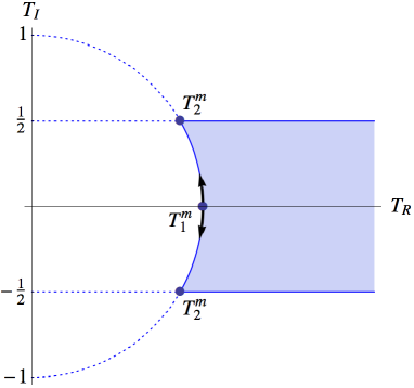 |
(See Fig. 1.)
To preserve the modular invariance of the whole Lagrangian, the scalar potential should be also modular invariant. Since the Kähler potential changes under the modular transformation as
| (12) |
the Kähler function and the scalar potential remain invariant if the superpotential transforms as
| (13) |
that is, the modular weight of should be . Using the the Dedekind eta function:
| (14) |
which is in the modular form with the modular weight , i.e., transforms as
| (15) |
we can construct a superpotential whose modular weight is as
| (16) |
Then, since the change of the Kähler potential in is canceled by the change of the superpotential, the scalar potential and the Lagrangian density for the effective field theory in 4D are now guaranteed to be modular invariant [8, 9].
Notice that the modular invariance prohibits to introduce a constant term in the superpotential. In the absence of the constant term, the cosine term, which introduces the deviation from the cosmological constant in the natural inflation, does not appear in the scalar potential. As a result, in the modular invariant inflation, we obtain a qualitatively different scalar potential from the usual axion inflation models with the natural inflation type potential (see, e.g., Ref. [10]).
2.2 Lagrangian and equations of motion
The Lagrangian density is given by
| (17) |
Taking the derivative of the Lagrangian density (17) with respect to and , we obtain the equations of motion as
| (18) | |||
| (19) |
where we defined
| (20) |
As is usual in inflation models from supergravity, the fields and have the non-canonical kinetic term.
2.3 Scalar potential
In our setup, we assume that the modulus fields and are the inflaton fields and the other fields are stabilized to constant values during inflation. Using
| (21) | |||
| (22) |
where denotes the derivative of with respect to , we can compute the scalar potential as
| (23) |
with
| (24) | |||
| (25) |
Since the fields are stabilized, and stay constant and serve free parameters. Here, we added a correction to the tree-level supergravity scalar potential, which may appear because of explicit supersymmetry breaking and/or loop effects.333Loop effects can be sizable, when there exist a sufficiently large number of modes, e.g. in the hidden sector[20]. The correction can be positive and negative and the value of depends on the detail of each model. In our setup, we assume that the correction is independent of 444 The modular invariance is unbroken unless develops its VEV. and can take both positive and negative values.
 |
The modular invariance implies that the values of at two points, which are related by the modular transformation, should coincide. Therefore, when at a point outside the fundamental domain takes a particular value, we can find another point inside the fundamental domain which has the same value of . As one may expect from this fact, the extreme values of the scalar potential can be found on the edge of the fundamental domain. Among the points on the edge of the fundamental region,
| (26) |
and
| (27) |
are mapped into themselves under with the identification of and . We find that the scalar potential takes extreme values at these points and . In particular, for , becomes the global minimum and for , becomes the global minimum 555We found that for , the global minimum may be located at another point near . In the rest of this paper, we do not discuss such a value of , but the gradient of for these values of is steep and hence it seems difficult to find a successful inflationary solution. For , both and become the global minimum. For the particular ansatz of and , which ensures the modular invariance, the absolute value in the square brackets in Eq. (23), i.e.,
vanishes at both and . Therefore, setting at the global minimum, we find the relation between , , and as
| (28) |
and obtain the scalar potential as
| (29) | |||
| (30) |
For , the global minimum is located at , i.e., and for , it is at , i.e., .
Notice that the scalar potential is determined solely by the three parameters , , and . The positive parameter determines the magnitude of the scalar potential and and determine the gradient of . In particular, whether an inflationary evolution can be realized or not is only determined by and , since can be absorbed into the normalization of the Hubble parameter (by using the -folding number as a time coordinate).
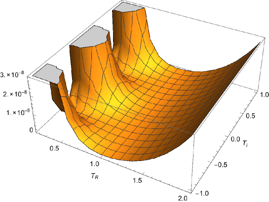
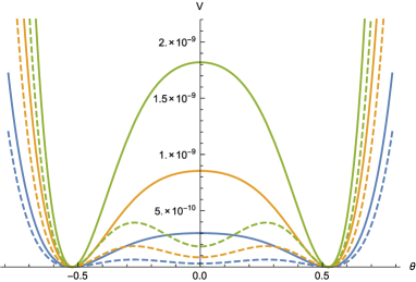
The scalar potential shows various features depending on the value of and also on the position in the space. In Fig. 2, we plot the scalar potential for , , and . Because of the invariance under , the potential in the direction of the axion becomes periodic. The scalar potential blows up in the limit and in the limit for some range of . As a consequence of the modular invariance, a region with a gentle slope can be found around , which is the edge of the fundamental region (see Fig. 1). This feature may become more obvious in the contour plot.
|
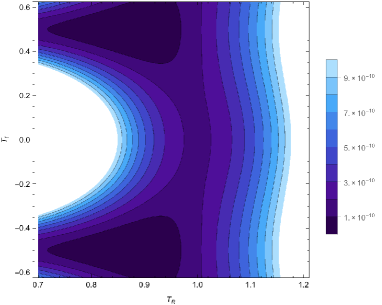
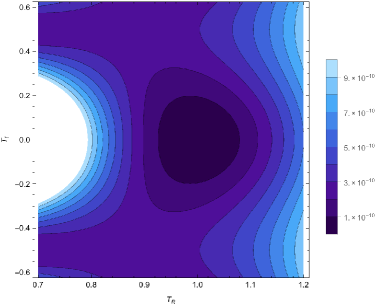
In Fig. 3, we show the contour plots of the scalar potential for and (Left) and (Right). For these values of , indeed, the gradient of around becomes comparatively shallow.
|
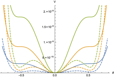
To capture the potential feature in more detail, in Fig. 4, we present the scalar potential on , i.e., . As described previously, the extreme values can be found at and . For , as we decrease , the point is transformed from the local maximum to the local minimum. In particular, the potential around becomes almost flat for . Meanwhile, for , is transformed from the inflection point to the local minimum. The potential for becomes nearly flat for .
2.4 Gross feature of : Hilltop potential
To get a better intuition on the gross feature of the scalar potential for on , where becomes almost flat namely around , we look for a simpler function which can approximate well. Expressing as , we consider the scalar potential for . Then, the modular invariance, namely the invariance under , requires the invariance under the change . Since for , keeping only the terms which are invariant under , we approximate the scalar potential as
| (31) |
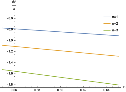
which agrees with the leading terms of the hilltop inflation during inflation. The value of which well approximates for each value of is presented in Fig. 5.
 |
Here, we determined , setting at , and determined , setting at . As is shown in Fig. 5, the dependence of can be approximately given by the following function
| (32) |
For , the curvature of the potential in the direction is positive and becomes the local minimum. Meanwhile, for , the curvature is negative and becomes the local maximum. This suggests that for we may find an inflationary solution which ends successfully. This will be verified in the next section.
3 Exploring inflationary solution
In this section, after we give the background equations of motion, we explore an inflationary solution with a sufficiently large -folding number.
3.1 Background evolution and slow-roll parameters
In the Friedmann-Robertson-Walker background, the field equations for and are given by
| (33) | |||
| (34) |
where is the Hubble parameter. As an action for gravity, we assume the Einstein-Hilbert action. Then, the Hamiltonian constraint equation gives the Friedmann equation:
| (35) |
Taking the time derivative of the Friedmann equation and using Eqs. (33) and (34), we obtain
| (36) |
We introduce the slow-roll parameters for and as
| (37) |
with . We also introduce the slow-roll parameter or the Hubble flow functions:
| (38) |
The slow-roll parameters and are related as
Using the slow-roll parameters, we obtain
| (39) |
When the magnitude of the slow-roll parameters stay small, i.e., , the field equations are given by
| (40) | |||
| (41) | |||
| (42) |
3.2 Case studies
3.2.1 Case1:
In Sec. 2.4, we examined the gross feature of the scalar potential around . As is suggested there, for , we indeed find an inflationary solution, which successfully ends. For , the gradient of the scalar potential is too steep to realize an inflationary evolution. For , where the effective mass becomes positive, the trajectory is either not realizing inflation (with a larger initial velocity) or approaching to the eternal de Sitter, being settled at the local maximum (with a smaller initial velocity).
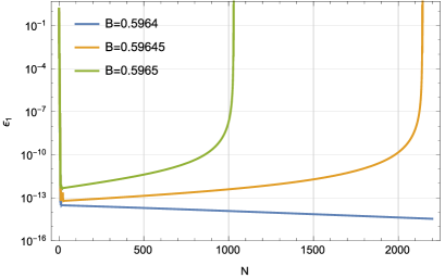
|
In Fig. 6, we plot the time evolution of for . Here, denotes the -folding number counted from the initial time . For , after the oscillation (in the direction of ), it approaches to the exact de Sitter solution. Meanwhile, for , after the oscillation, the modulus field starts to roll down the potential slowly all along . After a sufficiently long -folding, starts to oscillate again, terminating the slow-roll phase. In Fig. 6, we show the result in case we set the initial condition as
| (43) |
at . As expected from the fact that the potential around is approximated by the hilltop potential, which is small field, we need to fine tune the initial values of and . (To have an inflationary solution, and are preferred). We can vary the initial values of and in a broader region, since takes a minimum value at under the variation of around with fixed at .
During the inflationary stage, the trajectory almost traces the edge of the fundamental domain , changing the angle from towards . In this stage, the trajectory is predominantly determined by the axion and almost stays , i.e., . Then, the non-canonical kinetic term does not affect the evolution much, and the equation of motion is approximated by
| (44) |
Indeed, as shown in Fig. 7, (the blue solid line) agrees with (the orange dashed line) in a good precision.
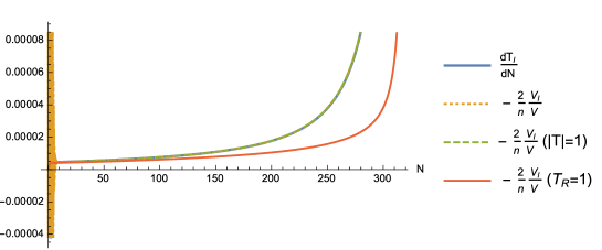 |
While the change of is tiny, this does not mean that we can neglect the curvature of the trajectory on by setting , because the potential gradient in the direction of is large. Therefore, in order to compute the accurate value of, say, , we need to take into account the variation of due to the tiny change of . As shown in Fig. 7, the value of evaluated for (the red solid line) sizably deviates from the one evaluated for the actual value of (the orange dashed line). By contrast, the value of evaluated for (the green dashed line) almost agrees with the actual value, which indicates the importance to take into account the curvature of the trajectory on .
When approaches to , the slow-roll evolution abruptly ends. In this stage, the deviation from the canonical kinetic term is onset and the trajectory depends on the two fields and . Therefore, in order to determine the total -folding number, we need to solve the two-field system with the non-canonical kinetic terms. Because of the non-linear velocity terms in the equations of motion for and , once and acquire non-negligible velocities, the slow-roll phase finishes much faster than the case with the same scalar potential , but with the canonical kinetic term.
 |
3.2.2 Case2:
For , becomes positive and for , becomes 0. For , one may simply identify with an explicit SUSY breaking uplift term. For , becomes the local minimum or the inflection point. We especially searched an inflationary solution which starts around and terminates around . However, all the solutions we found are either the one which does not embark an inflationary trajectory () or the one which approaches to the eternal de Sitter phase (). We leave an extensive study of this case for a future study. For , we did not find an inflationary solution with a sufficiently large -folding either.
As we have seen so far, requesting the modular invariance restricts a possible form of the scalar potential. As becomes larger, the scalar potential increases and for , the gradient of appears to be too steep to have an inflationary solution. The region where becomes nearly flat can be found only around . An inflationary solution with a successful exit was found only in the small parameter space of , i.e, and it is a small field inflation. We found that a large field inflation is hardly realized in moduli inflation with the modular invariance, which is crucially different from the axion inflation models where the modular invariance is broken 666 Small-field axion inflation also can be realized. See, e.g., Refs. [21, 22]..
4 Primordial perturbations
In the previous section, for , we found a new inflationary solution, whose gross potential during the slow-roll phase is approximately given by the hilltop type potential. In this section, we compute the primordial perturbations generated in this model and discuss the consistency with the CMB measurements.
4.1 Formulae of the primordial perturbations
As discussed in the previous section, the trajectory during inflation is mostly determined by the single degree of freedom , the angular direction. Following Gordon et al. [23], we define the adiabatic perturbation as the fluctuation in the direction of the background trajectory:
| (45) |
with
| (46) |
Performing the time coordinate transformation, we obtain the relation between the curvature perturbation on the slicing , , and on the flat slicing, , as
| (47) |
During inflation, since , which implies , and is suppressed due to the large mass, the curvature perturbation is predominantly determined by the fluctuation of the axion field as
| (48) |
where is the fluctuation of on the flat slicing. Using this formula, we can compute the power spectrum of simply by quantizing the canonically normalized scalar field
The primordial spectrum of , defined by
| (49) |
is given by the standard formula
| (50) |
Here and hereafter, we put the index on background quantities which are evaluated at the Hubble crossing time of the mode . Then, the spectral index and the tensor to scalar ratio are given by the standard formulae as
| (51) | |||
| (52) |
During inflation, since , the spectral index is almost determined only by at the Hubble crossing as
| (53) |
As seen in this subsection, the primordial spectrum in our model is superficially given by the same expression as the one for the canonical scalar field, because they are determined during the slow-roll phase, when the deviation from the canonical kinetic term is not effectively important.
4.2 Results
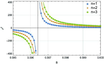
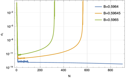
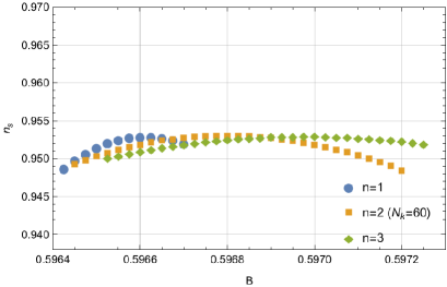
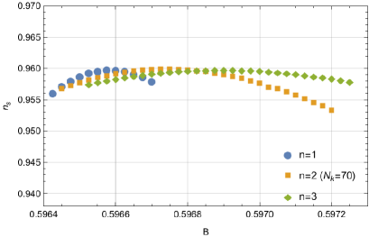
We compute the primordial spectrum for the values of which can yield the inflationary solution (). The result is presented in Fig. 9. We determined the end of inflation as the time when becomes and denotes the -folding number from the Hubble crossing time of the mode to the end of inflation. As we increase , at a certain value of , some of the slow-roll parameters with become larger than 1. In this paper, we only analyze the parameter space of where all of stay smaller than 1 during inflation, deferring the study of the case with the violation of the slow-roll condition for our future publication [24].
|
As we decrease the value of , the spectral index increases, approaching to the scale invariant spectrum. However, at a certain value of , the spectral index starts to decrease. The value of at which reaches the maximum, depends on . For a larger value of (in the right sides of two panels of Fig. 9), the spectral index is closer to 1 for than the one for and for smaller values (in the left sides), this becomes opposite.
This behaviour can be better understood by using the approximate expression of in the limit . Using Eqs. (31) and (32), we find that the curvature of the potential for the canonically normalized field is given by
| (54) |
As is mentioned previously, since is much smaller than , is determined by . Therefore, if the potential during inflation is all along given by the hilltop potential (31), the deviation from the scale invariant spectrum becomes smaller for a larger value of and for a smaller value of .
Obviously, this does not fully explain our result, which has the maximum value of and shows the more complicated dependence on . In addition, if the potential during inflation is accurately given by Eq. (31), the spectral index does not depend on , i.e., the spectral index can be determined without knowing when inflation ends. By contrast, our result significantly depends on . Because of that, there should be a non-negligible deviation from the hilltop potential (31), while it is useful simply to understand the gross feature of the scalar potential. In fact, while with become negligibly small in case the potential is precisely given by Eq. (31), in this model, with take non-vanishing values, letting vary in time.
For a larger value of and a smaller value of , the total -folding number becomes smaller (see Fig. 6) and the value of for a particular value of becomes smaller (as there was not enough time until to proceed towards the global minimum). Then, for a large value of and a small value of , tends to explore a region with a more gentle potential gradient at each , which makes the spectrum closer to the scale-invariant spectrum. The spectral index is determined as a result of the competition of these two effects. When the absolute value of the curvature of the gross potential given by Eq. (54) is small, the second effect is more important and the deviation from the scale invariance becomes larger for a smaller value of and a larger value of . Thus, as presented in Fig. 9, the deviation of the scale invariant spectrum has the minimum value in .
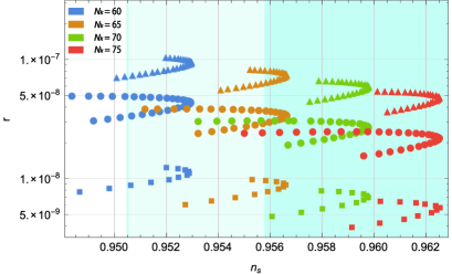
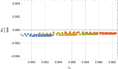
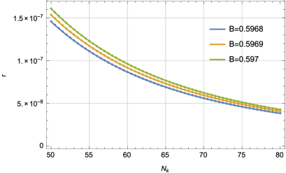
The left panel of Fig. 10 shows the -plot. The dark blue region is compatible with the Planck measurement in 68% CL and the light blue region is in 95% CL [13]. Here, we marginalized the running . Since is , the upper bound on the tensor to scalar ratio does not place any meaningful constraint on the parameter space of and . The amplitude of the primordial gravitational waves is rather small even among the small field models of inflation. This is because rapidly grows at the end of inflation due to the non-canonical kinetic term. Therefore, the value of for the CMB scales becomes much smaller than the one for the model with the same scalar potential and canonical kinetic term. In order to be compatible with the observations, the parameter should be fine tuned with 0.1 % level accuracy of its value. This may require a contrived setup in string theory, in particular in the presence of non-negligible radiative corrections, while the fine tuning problem is somehow common in small field models of inflation. In the right panel of Fig. 10, we show the running of the scalar spectral index. Since the slow-roll parameters at the Hubble crossing are sufficiently small, there is no enhancement of the running and the predicted value is obviously consistent with
| (55) |
|
|
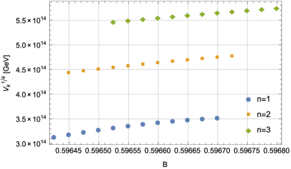
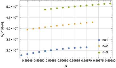
Inserting the value of the tensor to scalar ratio into
| (56) |
where is the amplitude of the scalar power spectrum [13] , we obtain the value of the scalar potential at the Hubble crossing, . (See Fig. 11.) Since the tensor to scalar ratio is extremely small as , the scale of the scalar potential is of , which is lower than the GUT scale. The Hubble scale during inflation is also low as [GeV]. Thus, the cosmological history is different from the one in large-field axion inflation with higher and .
|
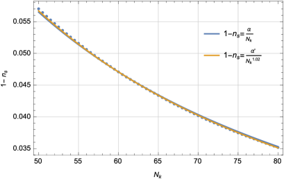
As was discussed in Refs. [25, 26], the CMB observations suggest that the spectral index is related to as
| (57) |
In such a case, solving
| (58) |
we can compute and the tensor to scalar ratio. Figure 12 shows that when the parameter is set to the ones which are compatible with the Planck measurements, the spectral index in this model is given by Eq. (57) in a good accuracy. For instance, for and , is given by , respectively. Then, using Eqs. (57) and (58) and integrating about , we obtain as
| (59) |
where is an integration constant. With an appropriate choice of , this expression reproduces the numerical result of as it should be (see the right panel of Fig. 12).
4.3 Reheating process and estimation of
The presence of the minimum value of is very important, because it gives a lower bound on to be compatible with the observations. The -folding should depend on the various physics after inflation and is given by [13, 27]
| (60) |
where and are the scale factor and the Hubble parameter at present and and are the energy densities at the end of inflation and at the time when the universe was thermalized after inflation, respectively. The parameter characterizes the effective equation of state during the oscillatory phase after inflation. When we insert the typical value of in this model and into the above expression, we obtain
| (61) |
Therefore, in particular, when the thermalization process is completed instantaneously, giving , this model is almost marginal at 95% CL.
Meanwhile, when and , a smaller value of will be predicted, which makes more unlikely to be compatible with the Planck data. In a single field model with the canonical kinetic term and a power-law scalar potential, requires the power of the scalar potential should be larger than 4. In our setup, the computation of will be more complicated because the evolution of the oscillatory phase is determined by the coupled two fields and with the non-canonical kinetic term. To calculate , we need to know the coupling between the inflaton and the standard model sector. In this model, since the inflaton is the modulus field, whose coupling to the standard model sector can be identified, will be predictable. Thus, by combining the information about the reheating, it may be possible to testify this model. A further study will be reported in our forthcoming publication [24].
5 Conclusion
In this paper, we investigated a phenomenological consequence of the modular invariance. In particular, we studied the moduli inflation with the Lagrangian which preserves the modular invariance. In this model, the minimum of the scalar potential, is located at the edge of the fundamental region for the explored values of . Setting the scalar potential at the global minimum to 0, we find that the Lagrangian density is determined only by the three parameters , , and . The modular invariance constrains the shape of the scalar potential (which is mainly determined by ) and the region with the flat potential was found only around .
A successful inflation model was found only in the restricted parameter region of , . The background trajectory during the slow-roll phase is almost determined by the axion, the imaginary part of the modulus field. Unlike in most of the successful axion inflation models, whose trajectory traces the large field periodic scalar potential, the scalar potential in this model is given by the hilltop potential with the small modulation, i.e., small field inflation. Then, the slow-roll inflation can take place without the super-Planckian excursion as in the natural inflation, which may give rise to a conflict to the UV completion of quantum gravity.
The predicted primordial gravitational waves are too tiny to be able to detect them in a near future. Then, it is unlikely to falsify this model only by examining the primordial perturbations. However, since the coupling of the modulus field to the standard model sector can be determined, the reheating temperature and the equation of state during inflation are potentially calculable in a self-complete way. Therefore, by studying possible values of , it may be possible to further examine the observational consistency of this this model. This result will be reported in our future study [24].
In this paper, we considered the simplest form of the superpotential which preserves the modular invariance. In Ref. [9], a generalization of the modular invariant model was explored. It may be interesting to see if this generalization allows us to find a new type of inflation. In the generalized setup, one may want to look for an inflation model where the global minimum can be set to by introducing a positive , since in such a case, we can identify with an explicit SUSY breaking uplift term. This investigation is left for a future study.
Acknowledgements
We would like to thank T. Higaki, K. Ichiki, and H. Otsuka for useful discussions. This project was initiated and completed under the support of Building of Consortia for the Development of Human Resources in Science and Technology. T. K. was supported in part by the Grant-in-Aid for Scientific Research No. 25400252 and No. 26247042 from the Ministry of Education, Culture, Sports, Science and Technology (MEXT) in Japan. D. N. is supported in part by MEXT Grant-in-Aid for Scientific Research on Innovation Areas, Nos. 15H05890. Y. U. is supported by JSPS Grant-in-Aid for Research Activity Start-up under Contract No. 26887018.
References
- [1] S. Hamidi and C. Vafa, Nucl. Phys. B 279, 465 (1987); L. J. Dixon, D. Friedan, E. J. Martinec and S. H. Shenker, Nucl. Phys. B 282, 13 (1987); T. T. Burwick, R. K. Kaiser and H. F. Muller, Nucl. Phys. B 355, 689 (1991); J. Erler, D. Jungnickel, M. Spalinski and S. Stieberger, Nucl. Phys. B 397, 379 (1993) [hep-th/9207049]; K. -S. Choi and T. Kobayashi, Nucl. Phys. B 797, 295 (2008) [arXiv:0711.4894 [hep-th]].
- [2] M. Cvetic and I. Papadimitriou, Phys. Rev. D 68, 046001 (2003) [Erratum-ibid. D 70, 029903 (2004)] [hep-th/0303083]; S. A. Abel and A. W. Owen, Nucl. Phys. B 663, 197 (2003) [hep-th/0303124]; D. Cremades, L. E. Ibanez and F. Marchesano, JHEP 0307, 038 (2003) [hep-th/0302105]; S. A. Abel and A. W. Owen, Nucl. Phys. B 682, 183 (2004) [hep-th/0310257].
- [3] D. Cremades, L. E. Ibanez and F. Marchesano, JHEP 0405, 079 (2004) [hep-th/0404229];
- [4] L. E. Ibanez and A. M. Uranga, “String theory and particle physics: An introduction to string phenomenology,” Cambridge University Press (2012). H. Abe, K. S. Choi, T. Kobayashi and H. Ohki, JHEP 0906, 080 (2009) [arXiv:0903.3800 [hep-th]].
- [5] V. S. Kaplunovsky, Nucl. Phys. B 307, 145 (1988) [Erratum-ibid. B 382, 436 (1992)] [hep-th/9205068].
- [6] L. J. Dixon, V. Kaplunovsky and J. Louis, Nucl. Phys. B 355, 649 (1991).
- [7] J. P. Derendinger, S. Ferrara, C. Kounnas and F. Zwirner, Nucl. Phys. B 372, 145 (1992).
- [8] S. Ferrara, N. Magnoli, T. R. Taylor and G. Veneziano, Phys. Lett. B 245, 409 (1990). doi:10.1016/0370-2693(90)90666-T
- [9] M. Cvetic, A. Font, L. E. Ibanez, D. Lust and F. Quevedo, Nucl. Phys. B 361, 194 (1991). doi:10.1016/0550-3213(91)90622-5
- [10] H. Abe, T. Kobayashi and H. Otsuka, JHEP 1504 (2015) 160 [arXiv:1411.4768 [hep-th]].
- [11] T. Higaki and F. Takahashi, JHEP 1503, 129 (2015) doi:10.1007/JHEP03(2015)129 [arXiv:1501.02354 [hep-ph]].
- [12] R. Kappl, H. P. Nilles and M. W. Winkler, Phys. Lett. B 753, 653 (2016) doi:10.1016/j.physletb.2015.12.073 [arXiv:1511.05560 [hep-th]].
- [13] P. A. R. Ade et al. [Planck Collaboration], arXiv:1502.02114 [astro-ph.CO].
- [14] K. Freese, J. A. Frieman and A. V. Olinto, Phys. Rev. Lett. 65, 3233 (1990).
- [15] E. Pajer and M. Peloso, Class. Quant. Grav. 30, 214002 (2013) doi:10.1088/0264-9381/30/21/214002 [arXiv:1305.3557 [hep-th]].
- [16] P. Svrcek and E. Witten, JHEP 0606, 051 (2006) doi:10.1088/1126-6708/2006/06/051 [hep-th/0605206].
- [17] J. E. Kim, H. P. Nilles and M. Peloso, JCAP 0501 (2005) 005 [hep-ph/0409138].
- [18] H. Abe, T. Kobayashi and H. Otsuka, PTEP 2015 6, 063E02 [arXiv:1409.8436 [hep-th]].
- [19] E. J. Copeland, A. R. Liddle, D. H. Lyth, E. D. Stewart and D. Wands, Phys. Rev. D 49, 6410 (1994) doi:10.1103/PhysRevD.49.6410 [astro-ph/9401011].
- [20] K. Choi, J. E. Kim and H. P. Nilles, Phys. Rev. Lett. 73, 1758 (1994) doi:10.1103/PhysRevLett.73.1758 [hep-ph/9404311].
- [21] M. Peloso and C. Unal, JCAP 1506, no. 06, 040 (2015) doi:10.1088/1475-7516/2015/06/040 [arXiv:1504.02784 [astro-ph.CO]].
- [22] T. Kobayashi, A. Oikawa and H. Otsuka, arXiv:1510.08768 [hep-ph].
- [23] C. Gordon, D. Wands, B. A. Bassett and R. Maartens, Phys. Rev. D 63, 023506 (2001) doi:10.1103/PhysRevD.63.023506 [astro-ph/0009131].
- [24] R. Iida, T. Kobayashi, D. Nitta, and Y. Urakawa, in preparation.
- [25] D. Roest, JCAP 1401, 007 (2014) doi:10.1088/1475-7516/2014/01/007 [arXiv:1309.1285 [hep-th]].
- [26] P. Creminelli, S. Dubovsky, D. Lopez Nacir, M. Simonovic, G. Trevisan, G. Villadoro and M. Zaldarriaga, Phys. Rev. D 92, no. 12, 123528 (2015) doi:10.1103/PhysRevD.92.123528 [arXiv:1412.0678 [astro-ph.CO]].
- [27] A. R. Liddle and S. M. Leach, Phys. Rev. D 68, 103503 (2003) doi:10.1103/PhysRevD.68.103503 [astro-ph/0305263].