Diffusion and transport in locally disordered driven lattices.

Abstract

We study the effect of disorder on the particle density evolution in a classical Hamiltonian driven lattice setup. If the disorder is localized within a finite sub-domain of the lattice, the emergence of strong tails in the density distribution which even increases towards larger positions is shown, thus yielding a highly non Gaussian particle density evolution. As the key underlying mechanism we identify the conversion between different components of the unperturbed systems mixed phase space which is induced by the disorder. Based on the introduction of individual conversion rates between chaotic and regular components, a theoretical model is developed which correctly predicts the scaling of the particle density. The effect of disorder on the transport properties is studied where a significant enhancement of the transport for cases of localized disorder is shown, thereby contrasting strongly the merely weak modification of transport for global disorder.

I Introduction

Driven lattice setups have long been one of the paradigmatic examples for the study of complex, out of equilibrium systems. In particular, their capability to transport particle ensembles in a controlled manner, even though all applied forces are zero mean valued, has stimulated considerable amounts of research and has under the label ’ratchet physics’ found direct applications in various physical settings Schanz et al. (2001, 2005); Serreli et al. (2007); Denisov et al. (2014); Liebchen and Schmelcher (2015); Reimann (2002); Hänggi and Marchesoni (2009). Noteworthy examples are Brownian or molecular motors Astumian and Bier (1994); Astumian (1997); Jülicher et al. (1997); Reimann (2002); Hänggi and Marchesoni (2009); Schmitt et al. (2015); Roth et al. (2015), or the controlled separation of particles or even living bacteria of different species Matthias and Müller (2003); Savel’ev et al. (2005); Bogunovic et al. (2012); Tahir et al. (2014). Since the uprising of cold atom physics, experiments have also been performed on atoms exposed to time dependently modulated optical standing waves where the controlled locomotion of atomic ensembles was realized Mennerat-Robilliard et al. (1999); Gommers et al. (2006); Schiavoni et al. (2003); Wickenbrock et al. (2012). Here, at temperatures well above the Bose Einstein transition temperature, it was shown how the atoms dynamics can be described reliably by means of a purely classical description Wickenbrock et al. (2012). Whereas most of the original works on ratchet physics are focused on the strongly damped or even over damped situation, in cold atom experiments, one could conveniently reach the Hamiltonian, that is the dissipation free, limit Wickenbrock et al. (2012). Another promising experimental realization of ratchets, which allow for a precise control over the systems parameters and thus are ideally suited to study the dissipation-less regime, are SQUIDs Weiss et al. (2000) where the phase of the macroscopic wave function is indeed described by a classical equation of motion Zapata et al. (1996); Spiechowicz et al. (2014). From a theoretical viewpoint, Hamiltonian ratchets have been analyzed comprehensively Flach et al. (2000); Schanz et al. (2001, 2005) and e.g. a sum rule was derived by which the systems asymptotic transport velocity can be deduced directly from the composition of the underlying mixed phase space Schanz et al. (2001).

Thereby, at the very heart of the analysis of Hamiltonian driven lattices, including the mentioned sum rule, is the apparent concept that different chaotic or regular components of the phase space are not mixed under time evolution. Recently however, setups have been proposed which allow for a conversion of particles from the systems chaotic layer into its regular components and vice versa Wulf et al. (2014); Liebchen et al. (2012); Petri et al. (2011); Wulf et al. (2012). In Wulf et al. (2014) this was achieved by introducing randomly placed impurities into an otherwise translationally symmetric arrangement of scatterers. Here, the collisions with the impurities were shown to induce hopping processes between different components of the unperturbed systems phase space. Even more, if the occurrence of impurities was restricted to a finite sized sub-domain of the lattice, an accumulation of particles into the regular structures of the unperturbed systems phase space was reported. Similarly, it was shown in Liebchen et al. (2012) how weak inter particle interactions again cause a conversion of particles into the regular structures of the phase space of the non interacting system. Here, it was also demonstrated that this subsequent filling of regular structures alter the systems transport properties, even leading to time dependent reversals of the transport direction. In a very different setting, it was also shown in Petri et al. (2011); Wulf et al. (2012) how a block lattice which is build up out of different domains allows for transitions between different components of the phase spaces of the individual blocks.

It is quite apparent that such conversion between the chaotic layer and regular structures lead to a significant modification of usual diffusive properties inherit to motion purely within the chaotic layer. However, a systematic investigation of the diffusive properties, or more generally speaking of the characteristics of the spatial particle density evolution, for systems with an inherent conversion between different components of a Hamiltonian mixed phase space is still missing, and is indeed the main subject of the present manuscript. To this end, we investigate a Hamiltonian system consisting of a temporally shaken lattice potential with additional randomly placed Gaussian barriers, acting as impurities. Similar to the results obtained in Wulf et al. (2014), we show that, by means of collisions with the impurity barriers, particles undergo conversion processes between different components of the mixed phase space of the unperturbed lattice. In cases were the occurrence of impurities is restricted to a finite domain of the lattice, we show that the spatial particle density develops strong tails with even increasing density towards larger positions. We provide a detailed analysis of the observed density evolution and propose a theoretical model, based on a decomposition of the entire particle ensemble into regular and diffusive sub-ensembles, which correctly predicts the scaling of the tails of the density. Furthermore, we argue how the inclusion of a localized disorder domain in a Hamiltonian ratchet may significantly enhance the directed current of the setup. Here, we give a modified version of the established sum rule of Hamiltonian ratchet transport Schanz et al. (2001) which incorporates the conversion from the chaotic layer into the regular structures of the unperturbed lattice.

Our manuscript is structured in the following way: In Sec. II we introduce the setup of a disordered lattice. Section III sums up the main results of disorder induced regular motion as described in Wulf et al. (2014). In Sec. IV we investigate the particle density evolution in a locally disordered lattice and derive a model which reproduces the correct scaling of the densities tails. Section V is devoted to the transport properties of the lattice and how they are influenced by the disorder. Finally, we conclude in Sec. VI.

II The disordered driven lattice.

We consider classical, non interacting particles of mass $m$ in one spatial dimension. Their dynamics is governed by the time-dependent Hamiltonian $H(x,p,t)=\frac{p^{2}}{2m}+V(x,t)$ with time $t$, position $x$, momentum $p$ and potential $V(x,t)$. Thereby, the particles are subjected to a laterally driven lattice potential, which is perturbed by randomly placed Gaussian barriers. That is the total potential $V(x,t)$ is given as the sum of a spatially periodic lattice potential, $V_{L}(x,t)$, with $V_{L}(x,t)=V_{L}(x+L,t)$ and a disorder potential $V_{D}(x,t)$. Specifically, the lattice potential $V_{L}(x,t)$ as well as the randomized term $V_{D}(x,t)$ are given by:

$$V(x,t) =V_{L}(x,t)+V_{D}(x,t)$$ (1)

$$=\mathcal{V}\cos^{2}[k(x-d(t))]+\mathcal{E}\sum_{n=-N_{D}}^{N_{D}}\chi_{n}\exp\left[-\left(\frac{x-d(t)-nL}{\sigma}\right)^{2}\right],$$

where $k\equiv\pi/L$ is the wave vector, $\mathcal{V}$ and $\mathcal{E}$ denote the strength of the lattice and the disorder potential and $\sigma$ is the Gaussian’s widths. $\chi_{n}$ is a randomized sequence of zeros and ones where we take the probability for a given element of $\chi_{n}$ to be one as $10\%$ and finally, $N_{D}$ fixes the extension of the disorder domain to $2N_{D}L$. Both the lattice and the perturbations are laterally driven according to the driving law:

$$d(t)=A\cos(\omega t)$$ (2)

with driving amplitude $A$ and frequency $\omega$ and hence, the Gaussians are centered in the minima of the lattice at all times (see Fig. 1 for an illustrative sketch of the system). It should be noted that, by transforming into the co-moving frame $x\rightarrow\tilde{x}=x-d(t)$, one can show straightforwardly that the transformed Hamiltonian $\tilde{H}$ describes a particle exposed to a static lattice which is of the form of $V(x,t)$ with $d(t)=0$ and an additional spatially constant oscillating force term $\propto\cos(\omega t)$.

In the following, we will investigate and compare three different scenarios: first, the unperturbed case with $\mathcal{E}=0$ and thus $V=V_{L}$. Second, the case of a globally disordered lattice as provided by Eq. (1) for $N_{D}\rightarrow\infty$ and finally, and this will actually be the main focus throughout this work, we will study the effects of a localized disorder region as realized by a finite, nonzero value of $N_{D}$. Quantities, such as the spatial or momentum densities will be labeled with superscripts “$0$”, “$GD$” or “$LD$” for the cases of no disorder, global disorder or local disorder respectively.

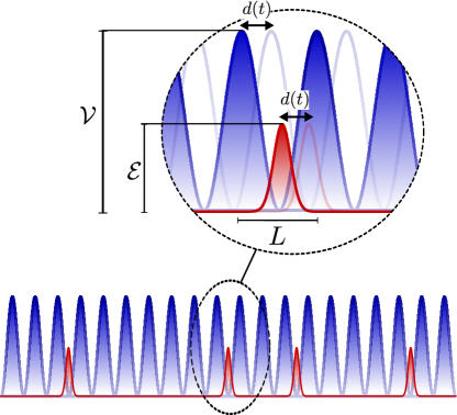
Figure 1: Snapshot of the lattice including the impurities in the form of Gaussian barriers which are placed randomly in the minima of the lattice. In the zoom, the lateral shaking of the entire system according to the driving law $d(t)$ is indicated together with the most relevant system parameters: the potential height of the lattice $\mathcal{V}$ and of the impurities $\mathcal{E}$ as well as the lattice spacing $L$.

III Unperturbed dynamics and disorder induced entering of regular structures.

Lets us very briefly recap the main features of the dynamics of a periodically driven, spatially periodic lattice, that is, the case for $\mathcal{E}=0$ in Eq. (1). Such a setup features a mixed phase space which can be visualized by a stroboscopic Poincaré surface of section (PSS). Here, the particles positions and momenta are recorded at times $0,T,2T,...$ with $T=2\pi/\omega$ being the temporal period. Furthermore, due to the systems spatial periodicity, the positions can be mapped back to the first unit cell. The PSS with the parameters as used throughout this work is shown in Fig. 2 and reveals the typical ingredients of a mixed phase space Lichtenberg and Lieberman (1992): a chaotic layer, ballistic islands embedded in it and invariant curves at higher energies. Of particular importance for what is to follow, are the two first invariant curves, which span the entire PSS and thus contain the chaotic layer towards higher and lower momenta, respectively. These will be referred to as FISCs in the following (First Invariant Surface spanning Curves). For a particle ensemble initialized at small velocities, the particles fill the chaotic layer ergodically, and the ensembles velocity distribution $\rho^{0}(v,t)$ is limited by the velocities corresponding to the motion on the two FISCs. Furthermore the ballistic islands constitute “forbidden” sub-manifolds of the phase space, leading to localized minima of $\rho^{0}(v,t)$ at velocities where the PSS features ballistic islands (see Fig. 3 (a)).

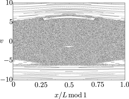
Figure 2: Poincaré section of the unperturbed system, that is for $\mathcal{E}=0$ in Eq. (1). Remaining parameters are $\mathcal{V}=4$, $k=0.79$, $\omega=3$ and $A=1$. Recording velocities and positions at different phases of the driving would reveal that the Poincaré section respects indeed the symmetry of the Hamiltonian of $x\rightarrow-x$, $v\rightarrow-v$ and $t\rightarrow t+\pi/\omega$.

We will now explain how the particle dynamics is altered by the inclusion of disorder, that is by setting $\mathcal{E}\neq 0$ in Eq. (1). In Wulf et al. (2014) it was demonstrated how randomized deviations from an otherwise spatially periodic system allow for a conversion process of particles from the chaotic layer into the regular structures. That is, the particles dynamics can still be described correctly by the phase space of the unperturbed system (henceforth referred to as PSUS), until a particle collides with one of the lattice impurities. At this point, the particle dynamics is no longer governed by the PSUS and a particle initially located within the chaotic layer of the PSUS may leave the scattering region of the impurity with phase space coordinates corresponding to a regular structure, e.g. a ballistic island, in the PSUS. Hence, such a particle would have undergone a conversion process from diffusive motion corresponding to the chaotic layer to regular motion in the ballistic island, where the opposite process, i.e. conversion from a ballistic islands into the chaotic layer of the PSUS, is equally possible. Indeed, the phase space distribution of an ensemble initially located within the chaotic layer of the PSUS and then evolving in the globally disordered system, reveals that the ballistic islands of the PSUS are now populated uniformly (see Fig. 3 (d)). This effect of a uniform filling of the phase space can also be seen in the velocity distribution $\rho^{GD}(v)$ (see Fig. 3 (b)), which does not show any substructure, such as local minima around distinct velocities which would hinge at unaccessible regular structures.

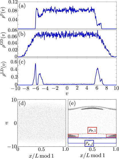
Figure 3: Velocity distributions $\rho(v)$ at time $t=10^{5}\times T$ for no disorder (a), global disorder (b) and local disorder with $N_{D}=5000$ (c). Phase space distribution at time $t=10^{5}\times T$ for global (d) and local (e) disorder. Disorder strength and width are $\mathcal{E}/\mathcal{V}=0.5$ and $\sigma/L=0.3535$; remaining parameters as in Fig. 2.

It was also shown in Wulf et al. (2014) that, in an arrangement of individual scatterers, a localization of the disorder to a certain domain causes the particles to even accumulate in the regular structures of PSUS. This holds also in our setup, as seen clearly in the phase space distribution for a disorder domain of $10^{4}$ lattice sites (i.e. $N_{D}=5000$) as shown in Fig. 3 (e) and also in the corresponding velocity distribution $\rho^{LD}(v)$ (Fig. 3 (c)), thus indicating the universality of the effect of disorder induced regular dynamics as reported in Wulf et al. (2014). We will now briefly sum up the two main mechanisms leading to this accumulation (a more detailed discussion can be found in Wulf et al. (2014)). Imagine a particle initialized at $x=0$ which leaves the disorder region for the first time. According to the discussion above, when the particle passes one of the edges of the disorder region at $x=\pm X_{D}\equiv\pm N_{D}\times L$, its phase space coordinates can either correspond to the chaotic layer of the PSUS or to one of its regular structures, i.e. to a ballistic island or one of the invariant curves above/ below the FISC. Since the ballistic islands as well as the invariant curves above/below the FISCs do not cross $v=0$, particles located within one of those structures while leaving the disorder region can never enter it again, and hence remain within the regular structure. On the contrary, if the particle crosses $X_{D}$ while moving within the chaotic layer, it may return to the disorder region after some time, and hence has another chance to be injected into a regular structure by collisions with the disorder barriers. The second mechanism for the accumulation is more subtle and hinges on the distribution of Lévy flight lengths of particles in different phase space structures. Here, one can show that, even within the disorder region, particles tend to dwell in the regular structures of the PSUS for comparably long times once they enter them. While following such a structure, the particles move ballistically through the lattice and hence overcome long distances, in particular much longer distances than they would overcome in the same time by the diffusive motion corresponding to the chaotic layer. It is thus more likely for a particle to reach $X_{D}$ while being within a regular structure than in the chaotic layer, which again adds to the accumulation effect.

IV Density evolution.

For the unperturbed lattice, the spatial density $\rho^{0}(x,t)$ of an ensemble which ergodically fills the chaotic layer may at least to some approximation be described by a Gaussian distribution whose width increases monotonically in time according to some diffusion coefficient. The density is in fact non Gaussian due to the trajectories tendency to become ”sticky” to regular structures and the associated build up of pronounced tails in $\rho^{0}(x,t)$. However, in particular close to the ensembles mean position a Gaussian remains a reasonable and often applied approximation. As discussed before, a localized disorder region leads to a conversion from diffusively moving particles into ballistically moving ones and hence, we can expect that Gaussian approximations of $\rho^{LD}(x,t)$, which are based on the assumption of a diffusive motion, break down entirely. In the following we discuss how the density in such a locally disordered lattice evolves in time. Furthermore we propose an insightful model, which is based on a decomposition of the ensemble into diffusively and regularly moving particles, and which is able to account for the main features in $\rho^{LD}(x,t)$.

In Fig. 4 we show the temporal evolution of the spatial density for an ensemble of $10^{4}$ particles with initial velocities $-0.1<v_{0}<0.1$ and initial positions $-10^{3}\times L<x_{0}<10^{3}\times L$ such that all particles are located well within the disorder order region ranging from $-5000\times L$ to $+5000\times L$. We very clearly see strong deviations from a diffusive, Gaussian spreading of $\rho^{LD}(x,t)$ at larger times. Here, strong tails in the distribution emerge which even increase for larger $x$. Furthermore, a dip in the density within the domain of disorder emerges as seen best in Fig. 4 (c). In the following we will show how both the tails in $\rho^{LD}(x,t)$ as well as the depletion within the disorder region can be understood.

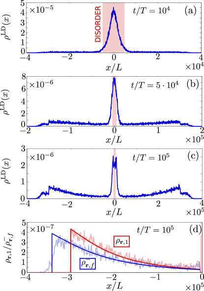
Figure 4: Density $\rho^{LD}(x,t)$ for a localized disorder domain (red) at times $t/T=10^{4}$ (a), $5\cdot 10^{4}$ (b) and $10^{5}$ (c). Parameters as in Fig. 3. (d) Decomposition of the density according to Eq. (11) at $t/T=10^{5}$ and for $x<0$. For $x<<0$, the density of the non regular particles, $\rho_{\textbf{nr}}$ is practically zero such that the entire density in the tails is given as: $\rho^{LD}\approx\rho_{\textbf{r},1}+\rho_{\textbf{r},f}^{-}$, where $\rho_{\textbf{r},1}$ contains all particles within the ballistic island at $v\sim-5.5$ of the PSUS and $\rho_{\textbf{r},f}^{-}$ all particles below the FISC at negative velocities (see also Fig. 3 (e)). The rough, shaded lines denote numerical results while the smooth lines show the densities according Eqs. (9), (10) with no free fit parameters.

Above, we argued that particles which leave the disorder region within a regular structure of the PSUS remain within this structure permanently, as they perform no further collisions with the impurity barriers and can thus not be converted back into the chaotic layer. Let us denote the total number of particles which are confined permanently to a regular structure of the PSUS as $N_{\textbf{r}}(t)$. That is, $N_{\textbf{r}}(t)$ includes all particles within a regular structure of the PSUS and which are located outside of the disorder region. The remaining particles will be denoted as $N_{\textbf{nr}}(t)$, which thus includes all particles within the disorder region and additionally particles outside the disorder which are located in the chaotic layer of the PSUS. The total number of particles $N$ is then given simply by $N=N_{\textbf{r}}(t)+N_{\textbf{nr}}(t)$. The same partition may be employed for the spatial density, hence we write the density of the total ensemble as:

$$\rho^{LD}(x,t)=\rho_{\textbf{r}}(x,t)+\rho_{\textbf{nr}}(x,t).$$ (3)

We will confirm later that $\rho_{\textbf{r}}$ describes the tails in $\rho^{LD}$ and we deduce the overall scaling of $\rho_{\textbf{r}}$ in the following.

By construction, the number of particles which are confined permanently to a regular structure of the PSUS, $N_{\textbf{r}}(t)$, cannot decrease, while particles associated to $N_{\textbf{nr}}(t)$ may be converted into permanently particles and thus add to $N_{\textbf{r}}(t)$. This conversion, in the sense of $N_{\textbf{r}}(t)$ and $N_{\textbf{nr}}(t)$ as defined above, may only occur at the instance when a particle leaves the disorder region and thus crosses the positions $\pm X_{D}$. It seems a reasonable assumption that the number of particles which cross $x=\pm X_{D}$ per time, and thus also the number of particles which are converted from $N_{\textbf{nr}}(t)$ to $N_{\textbf{r}}(t)$, is assumed proportional to the number of particles within the disorder region:

$$\frac{\partial}{\partial t}N_{\textbf{r}}(t)\approx\frac{\gamma}{T}\int_{-X_{D}}^{+X_{D}}\rho^{LD}(x,t)\,dx=\frac{\gamma}{T}\int_{-X_{D}}^{+X_{D}}\rho_{\textbf{nr}}(x,t)\,dx$$ (4)

with some proportionality constant $\gamma$ which denotes the fraction of the number of particles within the disorder region which is converted into regular structures per driving period $T$ and the second equality holds because, by definition, $\rho^{LD}=\rho_{\textbf{nr}}$ for $|x|<X_{d}$. We will show later, how the temporal evolution of $\partial_{t}N_{\textbf{r}}(t)$ links directly to the spatial dependence of the tails or the particle density at large positions. Note that the only time dependence in Eq. (4) is in the integrated density, i.e. in the number of particles which are located within the disorder domain at time $t$: $\int_{-X_{D}}^{+X_{D}}\rho_{\textbf{nr}}(x,t)\,dx$. In the following we deduce the scaling of this quantity which will then be used to derive the spatial dependence of the density outside the disorder region.

As a ”zeroth order” guess, one might assume that the part of the ensemble described by $\rho_{\textbf{nr}}(x,t)$, behaves as if there would be no disorder at all. This however, would neglect the conversion of particles into regularly moving ones which are described by $\rho_{\textbf{r}}$ and hence causes a particle loss in $\rho_{\textbf{nr}}$. Lets us now account for this loss effect by indeed assuming, that $\rho_{\textbf{nr}}$ is given by $\rho^{0}$, but with an additional particle loss given by the conversion into regular particles with rate $\gamma$ (cf. Eq. 4). The number of particles within the disorder region would then be given by:

$$\int_{-X_{D}}^{+X_{D}}\rho^{LD}(x,t)\,dx\approx(1-\gamma)^{t/T}\int_{-X_{D}}^{+X_{D}}\rho^{0}(x,t)\,dx,$$ (5)

where the factor $\int_{-X_{D}}^{+X_{D}}\rho^{0}(x,t)\,dx$ reflects that we assume that $\rho^{LD}$, within the disorder domain, behaves as if there would be no disorder at all and the factor $(1-\gamma)^{t/T}$ accounts for the fact that subsequently particles are removed from the disorder domain by being permanently converted into regular structures. For the density of the unperturbed system, we may furthermore assume a Gaussian: $\rho^{0}(x,t)=1/\sqrt{(}\pi)\sigma_{t}\exp[-(x/\sigma^{0}_{t})^{2}]$ where the time dependent width is assumed to be of the form $\sigma^{0}_{t}=L\sigma_{1}(t/T+\sigma_{2})^{\sigma_{3}}$ with three fit parameters $\sigma_{1,2,3}$. For the number of particles in the domain $|x|<X_{d}$ in the unperturbed system, this yields:

$$\int_{-X_{D}}^{+X_{D}}\rho^{0}(x,t)\approx\text{erf}\left(\frac{X_{d}}{\sigma^{0}_{t}}\right).$$ (6)

By explicitly simulating $\rho^{0}(x,t)$ we can justify this approximation and also fix the involved fit parameters $\sigma_{1,2,3}$ to $\sigma_{1}\approx 12.62$, $\sigma_{2}\approx 2.21\cdot 10^{4}$ and $\sigma_{3}\approx 0.645$. Inserting Eqs. (5) and (6) into Eq. (4) yields the increase of the number of regular particles:

$$\frac{\partial}{\partial t}N_{\textbf{r}}(t)=\frac{\gamma}{T}(1-\gamma)^{t/T}\text{erf}\left(\frac{X_{d}}{\sigma^{0}_{t}}\right).$$ (7)

Hence, the growth of the number of regular particles, $\partial_{t}N_{\textbf{r}}(t)$, decreases in time due to two effects: first, because of the diffusive spreading of the ensemble which transports the particles out of the disorder region and is described by the monotonically decreasing error function and second, because of the fact that the number of particles which are available to be converted into $N_{\textbf{r}}(t)$ decreases with every particle that has already been converted, which is accounted for by the exponentially decaying term.

So far we have not distinguished between the different regular structures of the PSUS (Fig. 2) in which particles may be converted, i.e. $\gamma$ describes the conversion rate into any one of them. However, in order to get the desired particle density, we need to do so and distinguished between the different regular structures. Therefor, we introduce individual rates for any of the accessible regular components $\gamma_{i}$, where each $\gamma_{i}$ accounts for one of the ballistic islands of the PSUS and two additional rates $\gamma^{\pm}_{\text{f}}$ account for the conversion into any of the regular curves above (below) the FISCs at positive (negative) velocities. Hence, the total rate, as used before, is given as

$$\gamma=\gamma^{+}_{\text{f}}+\gamma^{-}_{\text{f}}+\sum_{i}\gamma_{i}.$$ (8)

Thus, the change in the number of particles which are confined permanently within one of the ballistic islands is given by:

$$\frac{\partial}{\partial t}N_{\textbf{r},i}(t)=\frac{\gamma_{i}}{T}(1-\gamma)^{t/T}\text{erf}\left(\frac{X_{d}}{\sigma^{0}_{t}}\right).$$ (9)

and equivalently for the particles above (below) the FISCs denoted by $N^{\pm}_{\textbf{r},f}(t)$. Note that for the exponentially decaying term, the total conversion rate $\gamma$ is still the relevant quantity, while the overall prefactors of $\gamma_{i}$ or $\gamma^{\pm}_{\text{f}}$ are related to the specifics of the considered regular structure. The advantage of this decomposition is, that all particles associated to one of the $N_{\textbf{r},i}(t)$ have the same average velocity $\bar{v}_{i}$, which is the velocity of the regular islands central fixed point. Because of this, the spatial density, $\rho_{i}$, of particles within a given island can be calculated readily as:

$$\rho_{\textbf{r},i}(x,t) = \frac{\delta[x,\bar{v}_{i}]}{|\bar{v}_{i}|}\frac{\partial}{\partial t}N_{\textbf{r},i}\left(t-\frac{|x|-X_{d}}{|\bar{v}_{i}|}\right),$$ (10)

$$= \frac{\delta[x,\bar{v}_{i}]}{T|\bar{v}_{i}|}\gamma_{i}(1-\gamma)^{\tau/T}\text{erf}\left(\frac{X_{d}}{\sigma^{0}_{\tau}}\right)$$

where $\tau\equiv t-(|x|-X_{d})/|\bar{v}_{i}|$, $\delta[x,\bar{v}_{i}]$ equals one if $\text{sgn}(x)=\text{sgn}(\bar{v}_{i})$ and zero otherwise and we set $\partial_{t}N_{\textbf{r},i}(t)=0$ for $t<0$. For the particles above or below the FISCs the situation is more complicated since, here, every regular curve has a different velocity. However, we may use the average velocity $\bar{v}^{\pm}_{f}$ of the particles included in $N^{\pm}_{\textbf{r},f}(t)$, in which case Eq. (10) can be applied to obtain the corresponding densities $\rho^{\pm}_{\textbf{r},f}(x,t)$. The total density of regular particles is then given as:

$$\rho_{\textbf{r}}(x,t)=\rho^{+}_{\textbf{r},f}(x,t)+\rho^{-}_{\textbf{r},f}(x,t)+\sum_{i}\rho_{\textbf{r},i}(x,t).$$ (11)

In principle, the density of regular particles $\rho_{\textbf{r}}$ could be reproduced by means of Eqs. (10) and (11) if one would treat the conversion rates $\gamma_{i}$ and $\gamma^{\pm}_{f}$ as fit parameters. However, in order to demonstrate that our modeling of the density evolution indeed describes the physical processes correctly, we extract all conversion rates directly from our numerical simulations and thus fix the values of all involved parameters. Since our considered Hamiltonian is invariant under $x\rightarrow-x$, $p\rightarrow-p$, $t\rightarrow t+\pi/\omega$ we restrict ourselves to the regular structures with $\bar{v}<0$. The PSUS of our system features only a single notable ballistic island with a negative velocity (see Figs. 2 and 3 (e)). Hence the total density is decomposed in the following as: $\rho^{LD}(x<-X_{D})=\rho_{\textbf{r},1}+\rho^{-}_{\textbf{r},f}+\rho_{\textbf{nr}}$. In order to explicitly determine the conversion rates, we again consider the particle ensemble propagate in the setup containing localized disorder as before. At some fixed time $t=10^{5}$ we partition the ensemble into different parts depending on the particles coordinates in phase space (compare Fig. 3 (e)) and then count the number of particles in each part: Out of the entire ensemble of $N=5\times 10^{4}$ particles, we find $N_{1}=9681$ particles at positions $x<X_{d}$ within the ballistic island which are thus described by $\rho_{\textbf{r},1}$ and below the FISC are $N_{f}^{-}=9940$ particles (belonging to $\rho^{-}_{\textbf{r},f}$). Additionally, we get the total conversion rate $\gamma$ by using it as a fit parameter to the numerically obtain results of Eq. (5), yielding $\gamma\approx 10^{-5}$. By exploiting that $N_{1}/N_{f}^{-}=\gamma_{1}/\gamma_{f}^{-}$ and that $\gamma_{f}^{-}+\gamma_{1}=\gamma/2$ we get:

$$\gamma_{1}=\frac{\gamma}{2(1+N_{f}^{-}/N_{1})},\ \gamma_{f}^{-}=\frac{\gamma}{2(1+N_{1}/N_{f}^{-})},$$ (12)

yielding $\gamma_{1}\sim 2.47\times 10^{-6}$ and $\gamma_{f}^{-}\sim 2.53\times 10^{-6}$. The velocity of the ballistic island as well as the average velocity of the particles below the FISC are determined as: $\bar{v}_{1}\approx-5.70$ and $\bar{v}^{-}_{f}\approx-6.51$. Finally, we can compute the densities $\rho_{\textbf{r},1}$ and $\rho_{\textbf{r},f}^{-}$ according to Eq. (10) with no free parameter left. The resulting densities are shown in Fig. 4 (d) and show very good agreement to the numerically obtained ones. Note that the sudden drop to zero of $\rho_{\textbf{r},1}$ as seen both for the model as well as for the numerical data is simply at position $x=-(|\bar{v}_{1}|t+|X_{d}|)$, corresponding to the maximal distance that a particle can travel until time $t$ in a ballistic island with velocity $\bar{v}_{1}$. That this drop is smoothed out for $\rho_{\textbf{r},f}^{-}$, that is for particles below the FISC, is because, as mentioned before, theses particles all have slightly different velocities and we used their average velocity $\bar{v}^{-}_{f}$ in the theoretical model.

V Transport in globally and locally disordered lattices.

A typical question of interest in the non-equilibrium dynamics of driven lattices, is whether or not a setup is transporting, that is whether the mean velocity of a particle ensemble takes some non zero asymptotic value. In fact, the unperturbed lattice as studied above constitutes one the paradigmatic example for a Hamiltonian ratchet setup and is known to yield directed transport for a biharmonic driving law of the form:

$$d_{b}(t)=A_{1}\sin(\omega t)+A_{2}\sin(2\omega t+\phi),$$ (13)

if $\phi\neq 0,\pi$ Flach et al. (2000). Transport in these setups is usually studied for ensembles initialized at zero or small momenta and can be understood as a consequence of the asymmetrization of the systems chaotic layer around $v=0$ Schanz et al. (2001); Flach et al. (2000); Denisov et al. (2014). From the analysis performed in the previous section, it is clear however that even if the ensemble is started at zero momentum, it will not be restricted to the PSUSs chaotic layer as soon as disorder is included. Hence, it is an intriguing prospect to study the transport behaviour of the lattice in the presence of localized or global disorder, as e.g. the conversion into regular structures should lead to a violation of the sum rule of Hamiltonian ratchets Schanz et al. (2001).

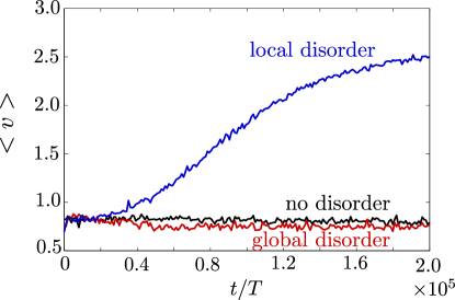
Figure 5: Mean velocities $<v>$ of particle ensembles for no disorder, global and local disorder as a function of time. Parameters of the lattice are the same as in Fig. 2. Parameters of the biharmonic driving law $d_{b}(t)$ are $A_{1}=1.0$, $A_{2}=0.5$, $\omega=3.0$ and $\phi=-7\pi/4$. For the local disorder case, the extension of the disorder domain was increased to $10^{5}\times L$.

In order to determine the transport, we initialize the particle ensembles as before and determine their evolutions for the same setups but with the biharmonic driving law $d_{b}(t)$ (cf Eq. (13)). The temporal evolution of the ensembles mean velocities are shown for the unperturbed lattice, as well as for localized and global disorder in Fig. 5. For the unperturbed case, we observe the usual behaviour of a Hamiltonian ratchet: very quickly (in fact on timescales hardly visible in Fig. 5), the ensemble fills the chaotic layer ergodically and the mean velocity fluctuates around the mean value of a trajectory in the chaotic layer, which we denote as $J^{0}$ in the following and which can be read off to be $\approx 0.8$ for the used set of parameters. For the globally disordered lattice, the mean velocity saturates against an asymptotic value of $J^{\text{GD}}$ which differs only slightly from its disorder free counter part $J^{0}$. In strong contrast, the local disorder leads to a significant increase of the mean velocity, which only slowly saturates towards its asymptotic value of $J^{\text{LD}}\approx 2.5$. In order to make this effect more apparent, we have increased the extension of the disorder domain as compared to the previous sections by a factor of $10$ to $10^{5}\times L$.

According to the sum rule of Hamiltonian ratchet transport, the asymptotic mean velocity of an ensemble initialized in the chaotic layer is given by the difference of the mean velocities of the FISCs at positive and negative velocities, minus the mean velocities of all ballistic islands weighted by their area in the systems PSS Schanz et al. (2001). In case of global disorder, the ballistic islands as well as the regular curves of the PSUS at higher energies become populated and thus may add to the directed transport. This process however, appears equally for regular structures at positive and negative velocities and thus the overall transport is not expected to change significantly. In this sense, one might say that the global disorder does not add to the desymmetrization of the system and hence has only little influence on the systems transport properties. For the localized disorder, this line of arguments holds as long as most particles are still located within the disorder region. Indeed we find, that $<v>$ follows the other two cases at early times $t/T\lesssim 0.2\cdot 10^{5}$ and deviates strongly only afterwards. The strong increase of the transport at later times can be understood straightforwardly by means of the analysis as performed before: At the edges of the disorder domain at $x=\pm X_{D}$, the ensemble is injected into the regular structures of the PSUS at some rates $\gamma_{i}$ or $\gamma_{f}^{\pm}$ and the number of particles within a given regular structure at a given time is assumed to be proportional to the number of particles which have crossed $x=\pm X_{D}$. In the previous section however, the ensemble was modeled simply as a Gaussian with some diffusive spreading described by its time dependent width $\sigma_{t}$. In a transporting systems, this description is insufficient as it neglects the overall drift of the ensemble within the disorder domain with a positive velocity of $J^{\text{GD}}\approx J^{0}$. Hence, more particles pass $x=+X_{D}$ per time as compared to $x=-X_{D}$ and thus conversion into regular structures with a positive velocity is enhanced. After some time, most particles are either converted permanently into regular structures of the PSUS or are transported diffusively out of the disorder domain and the mean velocity saturates against its asymptotic value $J^{\text{LD}}$. In analogy to the density (Eq. (11)), the transport can be written as:

$$J^{\text{LD}}=n_{\textbf{nr}}J^{0}+n^{+}_{\textbf{r},f}\bar{v}^{+}_{f}+n^{-}_{\textbf{r},f}\bar{v}^{-}_{f}+\sum_{i}n_{\textbf{r},i}\bar{v}_{i},$$ (14)

where the $n^{\prime}s$ denote the asymptotic ratios of the ensemble belonging to the respective part of the ensemble decomposition as introduced in section IV: $n_{\textbf{r},i}\equiv\lim_{t\rightarrow\infty}N_{\textbf{r},i}(t)/N$ and equivalently for particles above or below the FISCs. Note that by setting the transport velocity of the part of the ensemble which is not converted permanently to a regular structure to $J^{0}$, we have assumed that asymptotically all particles will have left the disorder domain and are thus governed by the PSUS with associated current $J^{0}$.

VI Conclusions.

We have studied how the dynamics of classical particles in a Hamiltonian driven lattice potential is altered by the inclusion of disorder. If the disorder is localized within a finite domain of the lattice, the particles are accumulated into the regular structures of the phase space of the unperturbed system. For this case, we show how the particle density inherits strongly pronounced tails, which at late times, even lead to an increase of the density towards larger positions. Hence, the localized disorder leads to a strong modification of the usual Gaussian like diffusion as observed in the unperturbed lattice. The observed particle densities are explained by means of a decomposition of the entire ensemble into regular and diffusive parts, where the regular part is decomposed further as a sum over all regular structures of the unperturbed phase space. We derive an approximate equation for the densities tail which accounts for the conversion from the diffusive part of the ensemble into the regular ones. All parameters of the resulting model can be fixed by numerical simulations, leading to a derived spatial dependence of the density with no free fit parameters left and which is shown to be in very good agreement with the full simulation.

Finally, we study the transport properties of a disordered lattice. While for global disorder, the asymptotic transport velocity is modified only slightly compared to the unperturbed lattice, we demonstrate that transport is increased significantly by the localized disorder. Here, we propose an extension to the usual sum rule of Hamiltonian ratchet transport which incorporates the effect of conversion processes from diffusive to regular parts of the unperturbed phase space as made possible by the inclusion of disorder.

References

- Schanz et al. (2001) H. Schanz, M.-F. Otto, R. Ketzmerick, and T. Dittrich, Physical Review Letters 87, 070601 (2001).
- Schanz et al. (2005) H. Schanz, T. Dittrich, and R. Ketzmerick, Physical Review E 71, 026228 (2005).
- Serreli et al. (2007) V. Serreli, C. F. Lee, E. R. Kay, and D. A. Leigh, Nature 445, 523 (2007).
- Denisov et al. (2014) S. Denisov, S. Flach, and P. Hänggi, Physics Reports 538, 77 (2014).
- Liebchen and Schmelcher (2015) B. Liebchen and P. Schmelcher, New Journal of Physics 17, 083011 (2015).
- Reimann (2002) P. Reimann, Physics Reports 361, 57 (2002).
- Hänggi and Marchesoni (2009) P. Hänggi and F. Marchesoni, Reviews of Modern Physics 81, 387 (2009).
- Astumian and Bier (1994) R. D. Astumian and M. Bier, Physical Review Letters 72, 1766 (1994).
- Astumian (1997) R. D. Astumian, Science 276, 917 (1997).
- Jülicher et al. (1997) F. Jülicher, A. Ajdari, and J. Prost, Reviews of Modern Physics 69, 1269 (1997).
- Schmitt et al. (2015) R. K. Schmitt, J. M. R. Parrondo, H. Linke, and J. Johansson, New Journal of Physics 17, 065011 (2015).
- Roth et al. (2015) J. S. Roth, Y. Zhang, P. Bao, M. R. Cheetham, X. Han, and S. D. Evans, Applied Physics Letters 106, 183703 (2015).
- Matthias and Müller (2003) S. Matthias and F. Müller, Nature 424, 53 (2003).
- Savel’ev et al. (2005) S. Savel’ev, V. Misko, F. Marchesoni, and F. Nori, Physical Review B 71, 214303 (2005).
- Bogunovic et al. (2012) L. Bogunovic, R. Eichhorn, J. Regtmeier, D. Anselmetti, and P. Reimann, Soft Matter 8, 3900 (2012).
- Tahir et al. (2014) M. A. Tahir, F. Nori, and B. B. Yellen, Journal of Applied Physics 115, 134902 (2014).
- Mennerat-Robilliard et al. (1999) C. Mennerat-Robilliard, D. Lucas, S. Guibal, J. Tabosa, C. Jurczak, J.-Y. Courtois, and G. Grynberg, Physical Review Letters 82, 851 (1999).
- Gommers et al. (2006) R. Gommers, S. Denisov, and F. Renzoni, Physical Review Letters 96, 240604 (2006).
- Schiavoni et al. (2003) M. Schiavoni, L. Sanchez-Palencia, F. Renzoni, and G. Grynberg, Physical Review Letters 90, 094101 (2003).
- Wickenbrock et al. (2012) A. Wickenbrock, P. C. Holz, N. A. A. Wahab, P. Phoonthong, D. Cubero, and F. Renzoni, Physical Review Letters 108, 020603 (2012).
- Weiss et al. (2000) S. Weiss, D. Koelle, J. Müller, R. Gross, and K. Barthel, Europhysics Letters 51, 499 (2000).
- Zapata et al. (1996) I. Zapata, R. Bartussek, F. Sols, and P. Hänggi, Physical Review Letters 77, 2292 (1996).
- Spiechowicz et al. (2014) J. Spiechowicz, P. Hänggi, and J. Luczka, Physical Review B 90, 054520 (2014).
- Flach et al. (2000) S. Flach, O. Yevtushenko, and Y. Zolotaryuk, Physical Review Letters 84, 2358 (2000).
- Wulf et al. (2014) T. Wulf, B. Liebchen, and P. Schmelcher, Physical Review Letters 112, 034101 (2014).
- Liebchen et al. (2012) B. Liebchen, F. K. Diakonos, and P. Schmelcher, New Journal of Physics 14, 103032 (2012).
- Petri et al. (2011) C. Petri, F. Lenz, B. Liebchen, F. Diakonos, and P. Schmelcher, Europhysics Letters 95, 30005 (2011).
- Wulf et al. (2012) T. Wulf, C. Petri, B. Liebchen, and P. Schmelcher, Physical Review E 86, 016201 (2012).
- Lichtenberg and Lieberman (1992) A. J. Lichtenberg and M. A. Lieberman, Regular and Chaotic Dynamics, Applied Mathematical Sciences, Vol. 38 (Springer, New York, NY, 1992).