Shortest Recurrence Periods of Forced Novae

Abstract

We revisit hydrogen shell burning on white dwarfs (WDs) with higher mass accretion rates than the stability limit, $\dot{M}_{\rm stable}$, above which hydrogen burning is stable. Novae occur with mass accretion rates below the limit. For an accretion rate > $\dot{M}_{\rm stable}$, a first hydrogen shell flash occurs followed by steady nuclear burning, so the shell burning will not be quenched as long as the WD continuously accretes matter. On the basis of this picture, some persistent supersoft X-ray sources can be explained by binary models with high accretion rates. In some recent studies, however, the claim has been made that no steady hydrogen shell burning exists even for accretion rates > $\dot{M}_{\rm stable}$. We demonstrate that, in such cases, repetitive flashes occurred because mass accretion was artificially controlled. If we stop mass accretion during the outburst, no new nuclear fuel is supplied, so the shell burning will eventually stop. If we resume mass accretion after some time, the next outburst eventually occurs. In this way, we can design the duration of outburst and interpulse time with manipulated mass accretion. We call such a controlled nova a “forced nova.” These forced novae, if they exist, could have much shorter recurrence periods than “natural novae.” We have obtained the shortest recurrence periods for forced novae for various WD masses. Based on the results, we revisit WD masses of some recurrent novae including T Pyx.

1. Introduction

A classical nova is a thermonuclear runaway (unstable hydrogen shell flash) event on a mass-accreting white dwarf (WD), which occurs if the mass accretion rate $\dot{M}_{\rm acc}$ is smaller than the stability limit $\dot{M}_{\rm stable}$ corresponding to the WD mass. Many theoretical works on hydrogen shell flashes have been published. In general, shorter decay times of novae are obtained for more massive WDs (e.g., Hachisu & Kato, 2006, 2010, 2014, 2015, 2016), and shorter recurrence periods correspond to more massive WDs with higher mass accretion rates (e.g., Prialnik & Kovetz, 1995; Wolf et al., 2013a, b; Kato et al., 2014).

If the mass accretion rate exceeds $\dot{M}_{\rm stable}$, nuclear burning is stable and no repeating shell flashes occur. This stability has long been studied in analytical and numerical works (Paczyński & Żytkow, 1978; Sienkiewics, 1975, 1980; Sion et al., 1979; Iben, 1982; Nomoto et al., 2007; Shen & Bildsten, 2007; Wolf et al., 2013a; Kato et al., 2014). The physical reason of stabilization was also presented by many authors (Sugimoto & Fujimoto, 1978; Fujimoto, 1982; Yoon et al., 2004; Shen & Bildsten, 2007, 2008). The border between the stable and unstable mass accretion rates is known as the stability line, i.e., $\dot{M}_{\rm stable}$, in the diagram of accretion rate versus WD mass (e.g., Nomoto, 1982).

There is another critical accretion rate, above which the optically thick winds occur (Hachisu et al., 1996; Hachisu & Kato, 2001). A hydrogen-rich envelope of a WD blows optically thick winds (Kato & Hachisu, 1994), instead of slowly expanding to a red-giant size (Nomoto, 1982). This critical mass accretion rate is dubbed as $\dot{M}_{\rm cr}$, which is about twice $\dot{M}_{\rm stable}$ (e.g., Kato et al., 2014).

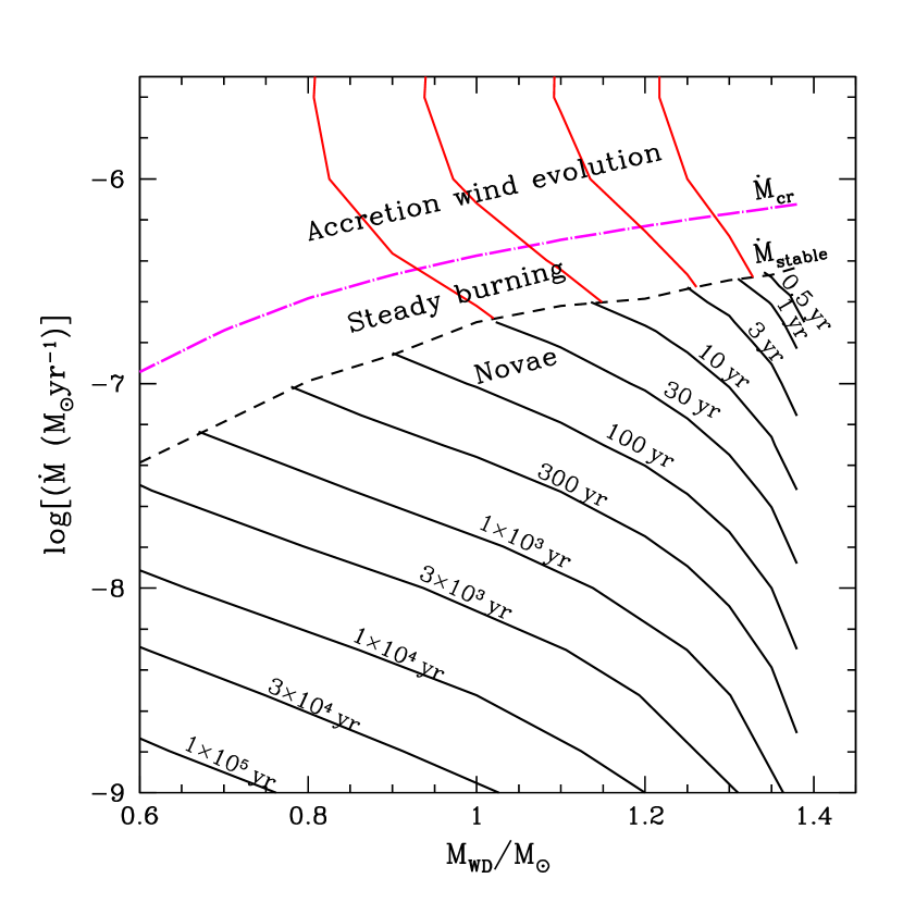
Figure 1.— Response of a WD envelope to mass accretion in the WD mass versus mass accretion rate. Above the stability line denoted by the black dashed line labeled $\dot{M}_{\rm stable}$, hydrogen shell burning is stable. Below the stability line (labeled “Novae”), shell flashes repeat with the recurrence period denoted by black solid lines. Above the critical line denoted by the magenta dash-dotted line, optically thick winds blow (labeled “Accretion wind evolution”). The data are taken from Figure 6 of Kato et al. (2014) for natural novae. We added red lines of recurrence periods of 1, 3, 10, and 30 yr for forced novae. See text for more details.

In summary, when the mass accretion rate $\dot{M}_{\rm acc}$ is less than the stability line, $\dot{M}_{\rm acc}<\dot{M}_{\rm stable}$, the nuclear burning is unstable and the WD undergoes a number of nova outbursts. If the mass accretion rate is between the two critical values, i.e., $\dot{M}_{\rm stable}<\dot{M}_{\rm acc}<\dot{M}_{\rm cr}$, the hydrogen shell burning is stable (see Figure 1). The accreted hydrogen-rich matter burns steadily on the WD at the same rate as the mass accretion rate. We suppose a binary configuration as illustrated in Figure 2; that is, the WD accretes matter from an accretion disk. Such a configuration has been used to explain supersoft X-ray sources (SSSs) (e.g., van den Heuvel et al., 1992; Schandl et al., 1997). If the mass accretion rate is larger than $\dot{M}_{\rm cr}$, i.e., $\dot{M}_{\rm acc}>\dot{M}_{\rm cr}$, optically thick winds blow from the surface of the envelope, and, at the same time, the WD accretes matter from the disk (see Figure 3). Hydrogen burning is stable and the accreted matter is partly burned into helium and accumulated onto the WD. The excess matter is lost by winds, with the mass-loss rate of $\dot{M}_{\rm wind}=\dot{M}_{\rm acc}-\dot{M}_{\rm nuc}$. Such a state was dubbed “accretion wind evolution” (Hachisu & Kato, 2001) and has been regarded as the state of luminous SSSs (also see Hachisu & Kato, 2003a, b). The most recent versions of the stability line and critical line for winds appeared in Figure 5 of Kato et al. (2014).

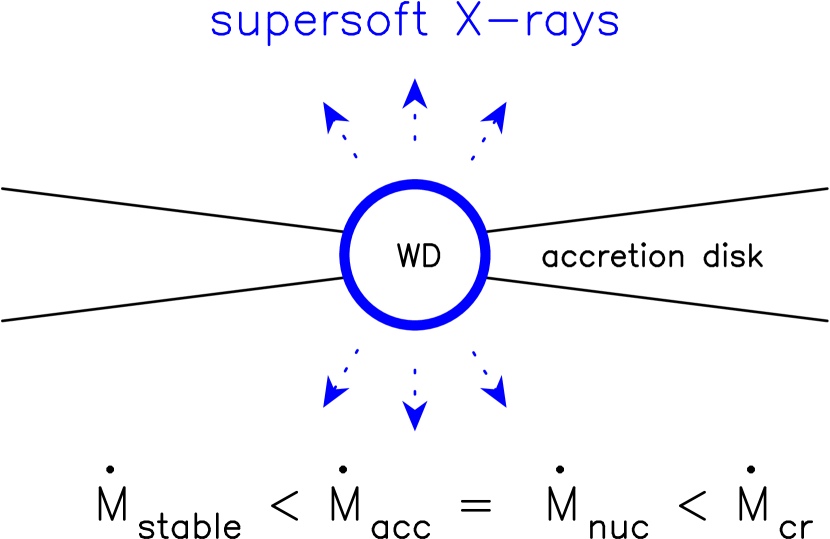
Figure 2.— Schematic configuration of steady hydrogen shell burning with no wind mass loss. The WD accretes matter from an accretion disk and burns hydrogen at the same rate as the accretion. No nova outburst occurs if the accretion rate is kept above the stability line. Such a configuration is often referred to as a persistent supersoft X-ray source.

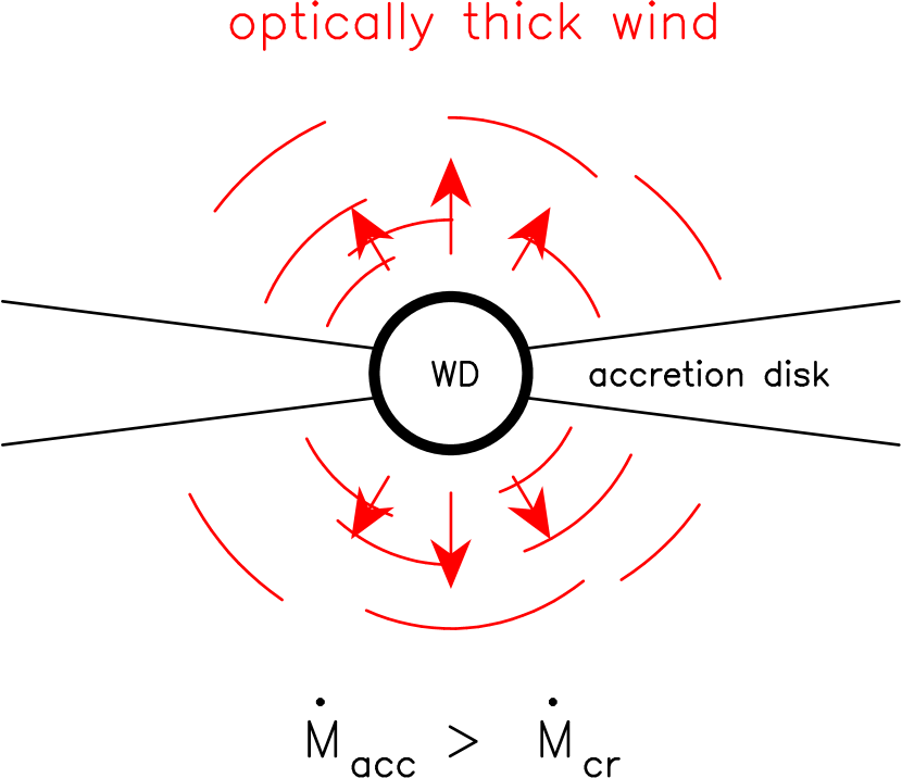
Figure 3.— Schematic configuration of accretion wind evolution. Hydrogen steadily burns on the WD. The WD accretes matter from a disk and blows excess matter into the wind. See text for more details.

To understand the nova cycle based on the above picture, we plot variations of envelope mass during one cycle of nova outburst in Figure 4, a model of steady-state envelope solutions on a $1.0~{}M_{\sun}$ WD (Kato & Hachisu, 1994; Hachisu & Kato, 2001). When the envelope mass reaches a critical value, hydrogen ignites to trigger a nova outburst (denoted by the upward arrow). The envelope expands to reach optical maximum (point C). The optically thick winds are accelerated so that the envelope mass decreases by wind mass loss ($\dot{M}_{\rm wind}$) and hydrogen burning ($\dot{M}_{\rm nuc}$). The envelope evolves down along with the black line with the photospheric temperature increasing. When the photospheric temperature reaches the OPAL opacity’s peak ($\log T$ (K) $\sim 5.2$), the optically thick winds cease (point B). We define this point as $M_{\rm env,cr}\equiv M_{\rm env}$(B), $\dot{M}_{\rm cr}=\dot{M}_{\rm nuc}$(B), and $\dot{M}_{\rm wind}$(B)$=0$, above which we have optically thick wind solutions. After that, the envelope mass still decreases because of nuclear burning. When it reaches point A, hydrogen nuclear burning diminishes and the WD cools down. There exist equilibrium hydrogen-burning envelope solutions below point A but they are unstable (see Figure 1 of Kato et al., 2014). We define this envelope mass as $M_{\rm env,min}\equiv M_{\rm env}$(A) and $\dot{M}_{\rm stable}=\dot{M}_{\rm nuc}$(A).

If the ignition mass is smaller than that at point B in Figure 4, i.e., $M_{\rm ig}<M_{\rm env,cr}=M_{\rm env}$(B), the nova reaches a point on the sequence between points A and B where no optically thick winds are accelerated. The envelope expands only slightly and the effective temperature does not decrease much, so it would be bright in the supersoft X-ray or UV band. It should be addressed that, if the accretion rate is high enough to be close to $\dot{M}_{\rm stable}$, the accretion to the WD during hydrogen shell burning makes the effective decreasing rate of the envelope mass smaller and, as a result, the nova-on (SSS) phase becomes significantly longer.

Point A for various WD masses describe the stability line $\dot{M}_{\rm stable}$ in Figure 1 while point B for each WD mass corresponds to the line of the critical mass accretion rate $\dot{M}_{\rm cr}$ for winds. If the mass-accretion rate $\dot{M}_{\rm acc}$ is between $\dot{M}_{\rm stable}$ and $\dot{M}_{\rm cr}$, i.e., $\dot{M}_{\rm stable}<\dot{M}_{\rm acc}<\dot{M}_{\rm cr}$, the hydrogen-rich envelope stays somewhere between A and B in Figure 4 and keeps a steady-state of $\dot{M}_{\rm nuc}=\dot{M}_{\rm acc}$ without wind mass-loss ($\dot{M}_{\rm wind}=0$). When the mass-accretion rate is larger than $\dot{M}_{\rm cr}$, i.e., $\dot{M}_{\rm acc}>\dot{M}_{\rm cr}$, the envelope stays somewhere between B and C (or above C) in Figure 4 and keeps a steady-state of $\dot{M}_{\rm wind}+\dot{M}_{\rm nuc}=\dot{M}_{\rm acc}>\dot{M}_{\rm cr}=\dot{M}_{\rm nuc}$(B).

These basic properties of mass-accreting WDs play essential roles in the evolution of binaries toward type Ia supernovae (SNe Ia). If the mass of a mass-accreting carbon-oxygen WD approaches the Chandrasekhar mass, carbon ignites to trigger an SN Ia explosion (Nomoto, 1982). The modern single degenerate (SD) scenario is based on the binary evolution theory in which both steady hydrogen shell burning (Figure 2) and accretion wind evolution (Figure 3) phases are taken into account in the evolutional paths to SNe Ia (e.g., Hachisu et al., 1996, 1999a, 1999b, 2010, 2012a, 2012b; Li & van den Heuvel, 1997; Langer et al., 2000; Han & Podsiadlowski, 2004).

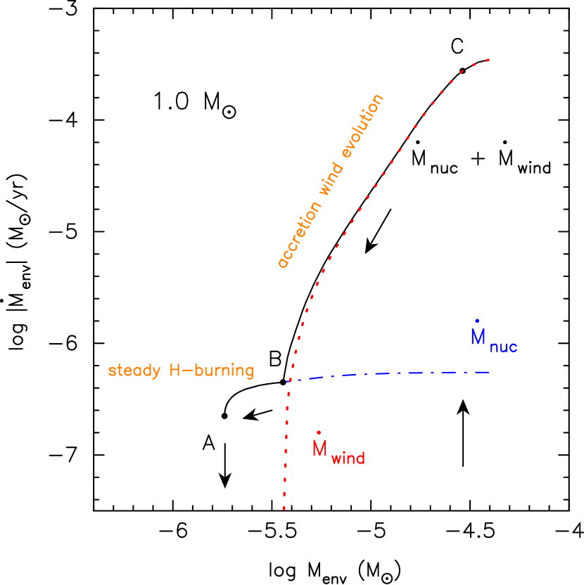
Figure 4.— Mass decreasing rate of the hydrogen-rich envelope ($-\dot{M}_{\rm env}=\dot{M}_{\rm wind}+\dot{M}_{\rm wind}$) versus envelope mass ($M_{\rm env}$) on a $1.0~{}M_{\sun}$ WD. The data are taken from the calculation of Kato & Hachisu (1994) for a $1.0~{}M_{\sun}$ WD with the envelope of solar composition. We assume steady state for the hydrogen-rich envelope on the WD. Hydrogen shell burning is stable when the envelope mass $M_{\rm env}$ is larger than $M_{\rm env,min}\equiv M_{\rm env}$(A) at point A, i.e., $M_{\rm env}>M_{\rm env,min}$. Optically thick winds blow when the envelope mass $M_{\rm env}$ is larger than $M_{\rm env,cr}\equiv M_{\rm env}$(B) at point B, i.e., $M_{\rm env}>M_{\rm env,cr}$. The mass decreasing rates are $\dot{M}_{\rm stable}=-\dot{M}_{\rm env}$(A) at point A, and $\dot{M}_{\rm cr}=-\dot{M}_{\rm env}$(B) at point B. For an envelope mass of the ignition mass $M_{\rm ig}$, the nova reaches point C, where $M_{\rm ig}=M_{\rm env}$(C), at optical maximum and then evolves down to point A through B along the steady-state sequence in the direction of arrows.

Some groups have recently claimed, however, that there is no steady hydrogen shell burning on mass-accreting WDs even above the stability line (e.g., Starrfield et al., 2012; Idan et al., 2013). Kato et al. (2014) elucidated the reason why they did not have steady hydrogen shell burning. Kato et al. showed two different evolutions of mass accretion. They started the mass accretion onto a WD (with no hydrogen burning) at a rate higher than the stability line and obtain a first shell flash. They stopped the mass accretion during the mass-loss phase. After some time elapsed (but with hydrogen shell burning still occurring), they restarted the mass accretion and obtained continuous shell burning (steady-state burning). However, they obtained repeated shell flashes if they did not start the mass accretion until hydrogen shell burning began to decay. These flashes are obtained only when they controlled the on/off epochs of mass accretion. Thus, one can obtain shell flashes above the stability line if one can control the on/off epochs of mass accretion. After Kato et al.’s (2014) paper was published, Hillman et al. (2015) further claimed that they did not find steady burning simply because their numerical code produced a series of shell flashes. Based on their time-dependent calculations, Hillman et al. (2015) concluded that steady hydrogen shell burning, on which Hachisu & Kato’s accretion wind evolution model depends, does not occur even above the stability line.

Motivated by such confusion, we study shell flashes above the stability line in a more systematic way. Here we call them “forced novae” after forced oscillation in physics. The forced novae occur only if we control the on/off epochs of mass accretion. In contrast, shell flashes naturally occur below the stability line, so we call them “natural novae.”

Forced novae may occur if the mass accretion is controlled by some mechanism in the binary system. For example, if the accretion disk is destroyed or if the mass transfer from the companion stops, the WD has some period without mass accretion until the accretion condition is recovered. For classical novae, which are considered to be systems below the stability line, this situation has already been discussed as “hibernation” (e.g., Shara et al., 1986).

Forced novae could have much shorter recurrence periods than those of natural novae. We obtain the shortest recurrence period of forced novae and compare them with the recurrence period of natural novae. These recurrence periods give an important constraint on the WD masses of recurrent novae. For example, for the Galactic recurrent nova U Sco, whose recurrence period is $t_{\rm rec}\sim 8$–12 yr, the WD mass is constrained to be $M_{\rm WD}>1.15~{}M_{\sun}$ from the recurrence periods of natural novae (see Figure 6 of Kato et al., 2014). In the same way, the minimum periods of forced novae can be used to constrain the WD mass. Using this constraint, we discuss the WD mass in T Pyx.

We organize the present paper as follows. In Section 2 we describe various forced nova evolutions using a time-dependent evolution code and in Section 3 we obtain the shortest recurrence periods of forced novae. We apply our results to various recurrent novae in Section 4 and constrain the WD mass of T Pyx by the shortest recurrence periods of forced novae. Finally we summarize our results in Section 5.

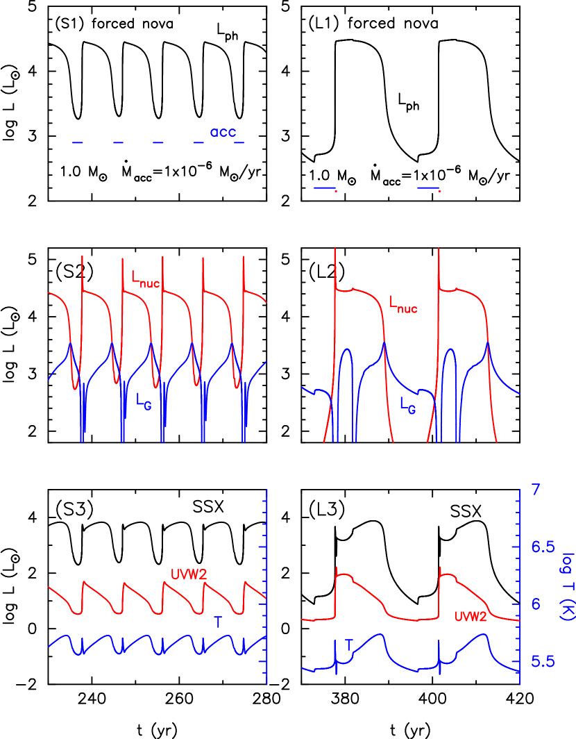
Figure 5.— Time-dependent calculations of shell flashes for forced novae on a 1.0 $M_{\sun}$ WD with a mass accretion rate of $1\times 10^{-6}~{}M_{\sun}$ yr^-1. Left panels (S1–S3, where “S” stands for short cycle): The last five cycles of our forced nova calculation with immediate resumption of accretion. (S1) Photospheric luminosity $L_{\rm ph}$. The accretion phase is indicated by the short horizontal blue lines labeled “acc.” The recurrence period is 9.2 yr. The on/off epochs of mass accretion are controlled to match the recurrence period with that of Idan et al. (2013). (S2) Nuclear luminosity $L_{\rm nuc}$ and gravitational energy release $L_{\rm G}$. The negative values of $L_{\rm G}$ are cut off by the lower bound of this figure. The photospheric luminosity in the interpulse phase is mainly supplied by $L_{\rm G}$. (S3) Photospheric temperature $T_{\rm ph}$, flux of supersoft X-rays (0.2–1 keV), and UV flux (1120–2640 Å) corresponding to the Swift $UVW2$ band. These luminosities are calculated from a blackbody assumption of the photospheric temperature and luminosity. Right panels (L1–L3, where “L” stands for long cycle): The same WD mass and mass accretion rate as those in the left panels, but with delayed on time of mass accretion. The recurrence period is 23.7 yr. See text for more details.

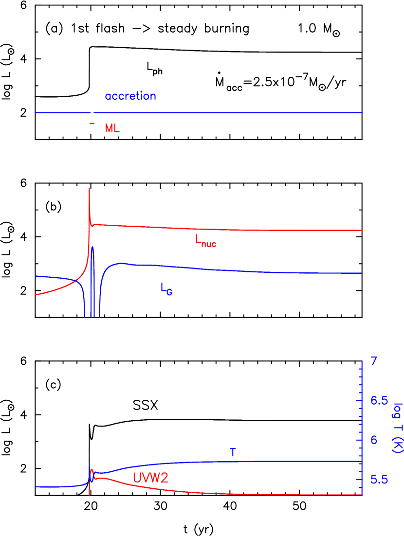
Figure 6.— Same as Figure 5, but for an immediate on time of mass accretion. The mass accretion rate is assumed to be $2.5\times 10^{-7}~{}M_{\sun}$ yr^-1. The WD undergoes a first shell flash and then settles down to steady-state hydrogen shell burning.

2. Time-Dependent Evolutions of Forced Novae

In principle, no nova outbursts occur above the stability line, i.e., $\dot{M}_{\rm acc}>\dot{M}_{\rm stable}$, in Figure 1 because nuclear burning is stable. However, there are two exceptions. One is the “first shell flash” (the first nova outburst) that occurs only once on the WD after it begins mass accretion. Suppose that a naked WD begins accretion. Hydrogen-rich matter accumulates on the WD. When it reaches the ignition mass, a hydrogen shell flash inevitably occurs. This is the first shell flash. If the mass accretion stays high as $\dot{M}_{\rm acc}>\dot{M}_{\rm stable}$, hydrogen shell burning becomes stable and never stops; i.e., the WD keeps bright. Thus, the first shell flash is the first and the last nova outburst for the WD. It never repeats nova outbursts. Then the binary configuration is either that in Figure 2 or that in Figure 3. The light curve for such a case has already been reported, e.g., in Figure 7(a) of Kato et al. (2014).

The other case is a forced nova. If we stop mass accretion at some epoch during shell flashes, the WD cannot keep steady hydrogen burning because of the shortage of nuclear fuel. The hydrogen shell burning eventually stops. Then, we resume mass accretion and have the next outburst. In this manner, we have successive nova outbursts by manipulating mass accretion on and off. The quiescent phase is determined by the epoch when we switch mass accretion on. In this way, we can freely design a nova outburst for an accretion rate above the stability line, that is, $\dot{M}_{\rm acc}>\dot{M}_{\rm stable}$, in Figure 1. This is the forced nova.

2.1. Numerical method

Evolution models of mass-accreting WDs were calculated by using the same Henyey-type code as in Kato et al. (2014). This code implements zoning based on the fractional mass ($q\equiv M_{r}/M$) in outer layers of the hydrogen-rich envelope, whereas zoning is based on $M_{r}$ in the rest of the interior including nuclear burning layers. In the outer layers the gravitational energy release per unit mass, $\epsilon_{\rm g}$, is calculated as (e.g., Neo et al., 1977)

$$\epsilon_{\rm g}\equiv-T\left(\partial s\over\partial t\right)_{M_{r}}=-T\left(\partial s\over\partial t\right)_{q}+T{d\ln M\over dt}\left(\partial s\over\partial\ln q\right)_{t},$$ (1)

where $M$ is the total mass of the WD, $M_{r}$ is the mass within the radius $r$, and $T$ and $s$ are the temperature and specific entropy, respectively. This zoning scheme with an off-center differencing for the equation of energy conservation (Sugimoto, 1970) works well for rapid evolution with mass accretion or decretion. Accretion energy outside the photosphere is not included.

The chemical composition of the accreting matter and initial hydrogen-rich envelope is assumed to be $X=0.7,~{}Y=0.28$, and $Z=0.02$. Neither convective overshooting nor diffusion processes of nuclei are included; thus, no WD material is mixed into the hydrogen-rich envelope. Because neutrino loss and electron conduction contribute very little to the total energy loss in the following calculations, we can approximate total energy conservation by

$$L_{\rm ph}=L_{\rm nuc}+L_{\rm G},$$ (2)

where $L_{\rm ph}$ is the photospheric luminosity, $L_{\rm G}$ is the total gravitational energy release rate calculated by using

$$L_{\rm G}=\int_{0}^{M}\epsilon_{\rm g}dM_{r},$$ (3)

and $L_{\rm nuc}$ is the total nuclear energy release rate calculated by using

$$L_{\rm nuc}=\int_{0}^{M}\epsilon_{\rm n}dM_{r},$$ (4)

with $\epsilon_{\rm n}$ the nuclear burning rate per unit mass.

For the initial WD model, we adopted an equilibrium model (i.e., “the steady-state models” of Nomoto et al., 2007), in which an energy balance is already established between heating by mass accretion and nuclear energy generation and cooling by radiative transfer and neutrino energy loss. This is a good approximation of the long time-averaged evolution of a mass accreting WD and we do not need to calculate many (thousands) cycles of shell flashes to relax thermal imbalance in the initial condition when we start from a cold WD. Starting from such an initial equilibrium state, the nova cycle approaches a limit cycle only after a few to several cycles (see, e.g., Kato et al., 2014, for more detail).

2.2. A Test: Comparison with Idan et al.’s result

We first check our numerical code by calculating shell flashes with the same parameters as those in Idan et al. (2013), i.e., the same WD mass ($M_{\rm WD}=1.0~{}M_{\sun}$) and mass accretion rate ($\dot{M}_{\rm acc}=1\times 10^{-6}~{}M_{\sun}$ yr^-1), and a very similar manipulation of mass accretion (on and off). This accretion rate is above the stability line. We plot the last five cycles of our forced nova calculation in Figure 5(S1)–(S3). The accretion phase is indicated by the short horizontal blue lines labeled “acc” in Figure 5(S1). The recurrence period is 9.2 yr. No mass ejection occurs. To compare with Idan et al.’s Figure 1, we see that our photospheric luminosity, $L_{\rm ph}$, in Figure 5(S1), recurrence period, and no mass ejection well reproduced Idan et al.’s results. Thus, we confirm that Idan et al.’s calculation describes a forced nova. Enlarging Figure 5(S1, S2) would reveals a very subtle kink in $L_{\rm ph}$ and $L_{\rm nuc}$ at the point of restarting accretion at $\log L_{\rm ph}/L_{\sun}=3.5$ $(\log L_{\rm nuc}/L_{\sun}\sim 3)$. This would probably correspond to small wiggles around $\log L/L_{\sun}\sim 3.3$ in Figure 1 of Idan et al. (2013), although the authors did not mention the cause of them. This further supports the fact that our manipulation of accretion to be similar to them.

Figure 5(S2) shows the nuclear luminosity, $L_{\rm nuc}$, and gravitational energy release, $L_{\rm G}$, for the same model as in Figure 5(S1). In the very early phase of the nova outbursts, nuclear burning produces a large flux, but most of this is absorbed into the bottom region of the hydrogen-rich envelope and the photospheric luminosity does not exceed the Eddington limit, so $L_{\rm ph}$ has a flat peak. The burning zone slightly expands to absorb the nuclear energy flux, which appears in the negative values of $L_{\rm G}$, although such negative values of $L_{\rm G}$ are cut off by the lower bound of the figure. The absorbed energy is gradually released in the later phase (positive values of $L_{\rm G}$). This energy release is a main source for the photospheric luminosity $(L_{\rm G}>L_{\rm nuc}>0)$ in the interpulse (quiescent) phase. Thus, the WD is still bright ($L_{\rm ph}>2000~{}L_{\odot}$) in the interpulse phase.

One of the important features of this forced nova is that the hydrogen-rich envelope does not expand so much. Thus, the photospheric temperature does not decrease to <300,000 K. Figure 5(S3) shows the photospheric temperature, $T_{\rm ph}$, supersoft X-ray (0.2–1 keV) flux, and UV band (1120–2640 Å) flux corresponding to the Swift $UVW2$ band. These luminosities are calculated by using a blackbody assumption from the photospheric temperature, $T_{\rm ph}$, and luminosity, $L_{\rm ph}$. They are very faint in the optical band, unlike classical novae. Thus, such objects are recognized, if they exist, as intermittent supersoft X-ray sources (SSSs). However, an anticorrelation between optical (high state) and supersoft X-ray (off state) in the intermittent SSSs, RX J0513.9$-$6951 and V Sge (e.g., Hachisu & Kato, 2003a, b), cannot be explained by these forced novae. Another important feature is the very high duty cycle (nuclear burning on $/$ cycle duration $=0.7$), i.e., 6.4 yr (on) + 2.8 yr (off) $=$ 9.2 yr (cycle duration). Such a high duty cycle is not consistent with those of recurrent novae as discussed in more detail in Section 4.

In connection to Figure 4, Idan et al.’s forced nova has a smaller ignition mass than the critical envelope mass, i.e., $M_{\rm ig}<M_{\rm env,cr}=M_{\rm env}$(B). After the onset of a shell flash, it reaches somewhere between A and B and moves leftward. This is consistent with the result that the nova has no wind mass-loss. When it reaches point A, nuclear burning extinguishes. The WD becomes dark and moves downward.

Recently, Hillman et al. (2015) also claimed that they did not obtain steady hydrogen burning. However, the light curves shown in Figures 1 and 5 of Hillman et al. indicate those are force nova models. In these light curves there are small jumps in luminosity around $\log L/L_{\sun}\sim 3.3$, which are signatures of re-starting matter accretion as seen in our Figure 5(L1). That is, they seems to re-start accretion too late to obtain steady burning.

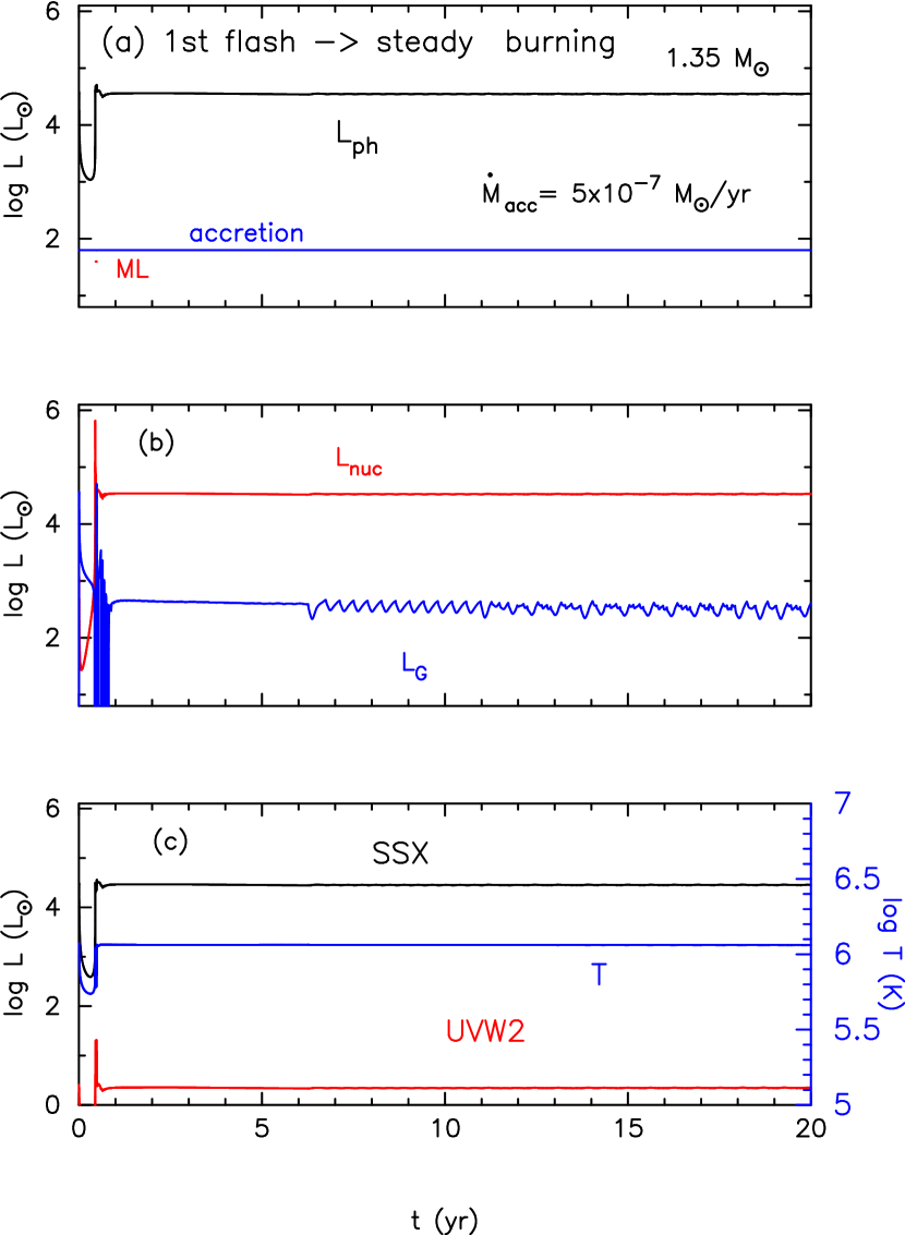
Figure 7.— Same as Figure 6, but for a WD mass of $1.35~{}M_{\sun}$ and a mass accretion rate of $5\times 10^{-7}~{}M_{\sun}$ yr^-1. The WD undergoes a first shell flash and then settles down to steady-state hydrogen shell burning.

2.3. First shell flash followed by steady hydrogen shell burning

Figure 6 shows an example of our calculation of the first shell flash on a $1.0~{}M_{\sun}$ WD with a mass accretion rate of $\dot{M}_{\rm acc}=2.5\times 10^{-7}~{}M_{\sun}$ yr^-1, which is located in the middle of the steady hydrogen-burning zone in Figure 1 ($\dot{M}_{\rm stable}<\dot{M}_{\rm acc}<\dot{M}_{\rm cr}$). This first shell flash occurs 20 yr after the start of mass accretion. The accreted matter is $\log M_{\rm env}~{}(M_{\sun})\approx-5.3$, which exceeds the critical envelope mass for wind mass loss, i.e., $M_{\rm env}>M_{\rm env,cr}=M_{\rm env}$(B), in Figure 4. So, we have mass loss during a short period (denoted by the orange line labeled “ML”). Another example is an accreting 1.35 $M_{\sun}$ WD with $\dot{M}_{\rm acc}=5\times 10^{-7}~{}M_{\sun}$ yr^-1, as shown in Figure 7 (the same model as in Figure 7 of Kato et al., 2014). It has a first shell flash 0.5 yr after the onset of accretion and maintains steady burning.

In this way, the first shell flash always occurs if we start the mass accretion onto a naked WD for any accretion rate above the stability line. Of course, this does not mean that the hydrogen shell burning is unstable. We note that Starrfield et al.’s (2012) claim of the absence of steady burning seems to be misguided from their calculations up to the first flash; they didn’t continue the calculation after the first flash.

In the models of Figures 6 and 7, we resume mass accretion just after the wind mass loss stops, i.e., before the hydrogen burning extinguishes (before it reaches point A in Figure 4). Hydrogen shell burning continues. The accreted matter burns steadily at the same rate as the mass accretion. The luminosity is constant with time in a balance of $L_{\rm ph}\approx L_{\rm nuc}$, and the envelope mass is also constant with time. Hydrogen shell burning is stable and never stops as long as we maintain the mass accretion as indicated by the horizontal blue lines in Figures 6(a) and 7(a). A helium layer develops underneath the hydrogen burning shell. A helium shell flash occurs when the mass of the helium layer becomes large enough.

We suppose that these binaries are in the steady state described in Figure 2. The photospheric temperature of a WD is high enough to emit supersoft X-rays. Such an object could be recognized as a persistent luminous supersoft X-ray source (e.g., van den Heuvel et al., 1992; Kahabka & van den Heuvel, 1997).

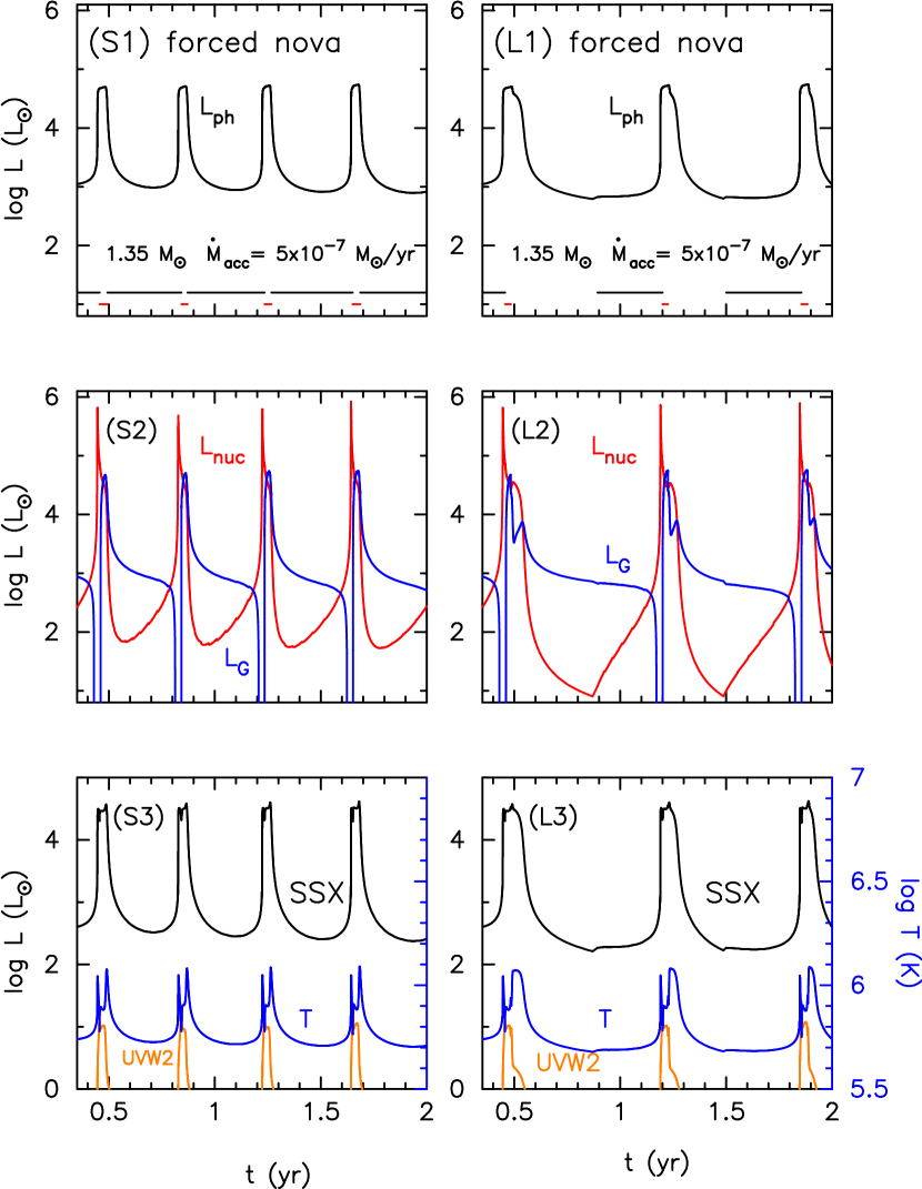
Figure 8.— Shell flashes on a $1.35~{}M_{\sun}$ WD with a mass accretion rate of $5\times 10^{-7}~{}M_{\sun}$ yr^-1. If we resume the mass accretion immediately after hydrogen shell burning ends, as indicated by the horizontal black lines, the next shell flash begins every 0.42 yr in the left panels (S1–S3). If we postpone the mass accretion until $L_{\rm nuc}<10~{}L_{\sun}$, we get a longer recurrence period of 0.67 yr, as in the right panels (L1–L3). Horizontal black and red lines in panels (S1) and (L1) denote accretion phase and mass-loss phase, respectively. These two forced nova models are taken from Kato et al. (2014).

2.4. Forced novae: Manipulated mass accretion

The on/off epochs of mass accretion can be designed to control the recurrence period even for the same mass accretion rate and WD mass. If we continue mass accretion during the bright $L_{\rm ph}$ phase of the first shell flash, we obtain continuous hydrogen shell burning, which never stops as long as we continue mass accretion (until a helium shell flash occurs). However, if we stop at the beginning of a flash and resume mass accretion after hydrogen burning extinguishes, we obtain successive shell flashes. In this case, a later on time of mass accretion results in a longer recurrence period.

Figures 5(L1)–(L3) demonstrate an example of designed mass accretion. For the same WD mass and mass accretion rate as those of Figures 5(S1)–(S3), we can get a longer recurrence period of 23.7 yr by omitting mass accretion for 7 yr. The outburst amplitude is larger than in the case of Figure 5(S1) because of the cooling during the longer interpulse phase (compare Figure 5(S2) with Figure 5(L2)). Since the ignition mass in Figure 5(L1) is larger than that in Figure 5(S1), the outburst duration is longer in Figure 5(L1). The supersoft X-ray flux in the interpulse phase is lower in Figure 5(L3) than in Figures 5(S3). In this way, we can design the recurrence period by changing the onset time of mass accretion.

Figures 8(S1)–(S3) and (L1)–(L3) depict other examples, that is, the same models as in Figures 7(b) and 7(c), respectively, of Kato et al. (2014), showing successive shell flashes for a forced nova on a $1.35~{}M_{\sun}$ WD with a mass accretion rate of $5\times 10^{-7}~{}M_{\sun}$ yr^-1. In Figure 8(S1), we assume immediate resumption of mass accretion after hydrogen shell burning begins to decay, as shown in the horizontal black (accretion) and red (mass loss) lines. If we restart the mass accretion a bit later, as shown in Figure 8(L1), we get a longer recurrence period. In this case, the nuclear burning region cools much more than in the case of Figure 8(S1), so $\log L_{\rm nuc}~{}(L_{\sun})$ dropped to 1.0 in the interpulse phase, a tenth of that in the case of Figure 8(S2). In contrast, the photospheric luminosity $\log L_{\rm ph}$ in Figure 8(L1) does not decrease much in the interpulse phase but is almost the same as that in the case of Figure 8(S1), because it is supplied by the gravitational energy release $\log L_{\rm G}$. The duration of outbursts is longer in Figure 8(L1) than in Figure 8(S1) because the ignition mass is larger in Figure 8(L1) owing to the cooling effect during the longer interpulse duration. In both cases, forced novae may be observed, if they exist, as an intermittent supersoft X-ray source. However, the optical and soft X-ray model light curves in Figures 5 and 8 cannot explain the anticorrelation between the optical high state and the supersoft X-ray off state observed in RX J0513.9$-$6951 and V Sge.

Figure 9.— Recurrence periods for various mass accretion rates on a 1.0 $M_{\sun}$ WD. Black dots indicate the case in which mass loss occurs in the early phase of the shell flash, while open circles indicate the case of no mass loss. The minimum value is 6.4 yr for $\dot{M}_{\rm acc}=5.0\times 10^{-6}~{}M_{\sun}$ yr^-1.

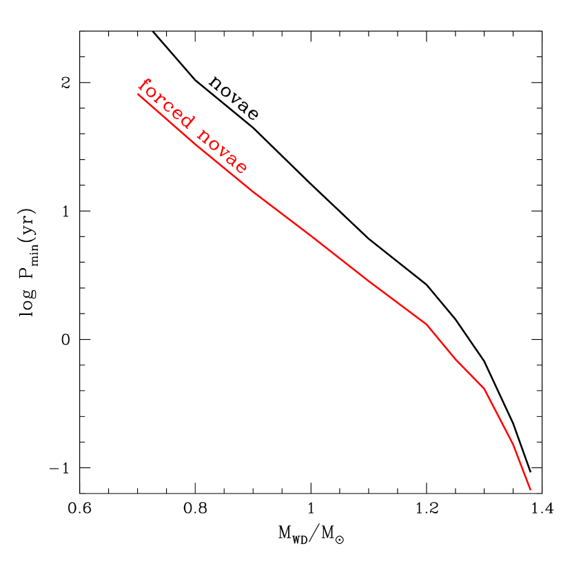
Figure 10.— Shortest recurrence periods for various WD masses. The red line indicates the minimum recurrence period of forced novae. The black line indicates the minimum recurrence period of natural novae, which is taken from Kato et al. (2014). See text for more details.

3. Shortest Recurrence Periods of Forced Novae

Forced novae could have shorter recurrence periods than natural novae do. Because the recurrence period is a useful indicator of the WD mass of a recurrent nova, we obtain the minimum recurrence periods of forced novae.

As shown in Figures 5 and 8, we obtain the shortest recurrence period for a given WD mass and mass accretion rate if we switch on the mass accretion immediately after a shell flash ends (i.e., when hydrogen shell burning begins to decay). Here, we identify the end of the shell flash as when the photospheric luminosity decays by a factor of 3 from that at the knee in the HR diagram. For a $1.0~{}M_{\sun}$ WD, the switch-off luminosity is $\log L_{\rm ph}~{}(L_{\sun})=4.2$ and the switch-on luminosity is $\log L_{\rm ph}~{}(L_{\sun})=3.7$.

Figure 9 shows the recurrence periods of a $1.0~{}M_{\sun}$ WD for various mass accretion rates. For low accretion rates, the recurrence period decreases as the accretion rate increases because the accretion time to ignition mass becomes shorter. For a very large mass accretion rate, the recurrence period increases because additional mass is accreted after the ignition (making the duration of hydrogen burning longer) before the luminosity increases to the switch-off luminosity. We obtain the shortest recurrence period of 6.4 yr at $\dot{M}_{\rm acc}=5\times 10^{-6}~{}M_{\sun}$ yr^-1 for a $1.0~{}M_{\sun}$ WD.

The recurrence period of a nova, $t_{\rm rec}$, is composed of

$$t_{\rm rec}=t_{\rm nova-off}+t_{\rm nova-on},$$ (5)

where $t_{\rm nova-off}$ is the duration of the quiescent phase (accretion phase, that is, hydrogen burning off) and $t_{\rm nova-on}$ is the duration of nova outburst (during which hydrogen shell burning is occurring). In classical novae, $t_{\rm nova-on}$ is much shorter ($\sim$$1$ yr or so) than $t_{\rm nova-off}$ ($10^{3}$–$10^{5}$ yr or so), so we may neglect it. Although neglecting $t_{\rm nova-on}$ is a very good approximation for longer recurrence periods, slight deviations are appreciable for recurrence periods of 1 and 3 yr in Figure 1.

In this manner, we obtained the recurrence periods of forced novae for various WD masses and mass accretion rates and plotted them in the mass accretion rate versus WD mass diagram in Figure 1 by using red lines for $t_{\rm rec}=1$, 3, 10, and 30 yr. The red lines (forced novae) for recurrence periods of 1 and 3 yr shift slightly from the corresponding black lines (natural novae) at the stability line (dashed line). The shifts indicate that the recurrence period of a forced nova for a given $M_{\rm WD}$ and $\dot{M}_{\rm acc}$ is slightly longer than that of the corresponding natural nova. This comes from the fact that recurrence times of natural novae (adopted from Kato et al., 2014) were calculated by neglecting the $t_{\rm nova-on}$ time, while recurrence periods of forced novae are obtained by calculating full cycles of novae.

We summarize the shortest recurrence periods of forced novae for various WD masses as shown by the red solid line in Figure 10. In the region below the red line, we do not have corresponding objects. In the region above the red line, forced novae can exist if we introduce some switch on/off mechanism. In general, for a given WD mass, a longer recurrence period is obtained if we interrupt the mass accretion for a longer time. Thus, the duty cycle is higher for a shorter recurrence period.

The shortest recurrence periods of natural novae are obtained near the stability line. We also plot the minimum value by the black line in Figure 10. The values are taken from the recurrence period on the line of $\dot{M}_{\rm stable}$ in Figure 1 (with the original value being in Figure 6 of Kato et al., 2014). In the region below the black line, we have no natural novae. Above the line, shorter recurrence periods correspond to recurrent novae. The duty cycle is also higher for a shorter recurrence period. These black and red lines clearly show that the minimum recurrence period of a forced nova is always shorter than that of a natural nova.

4. Discussion

Now, we compare our calculated recurrence periods with those of recurrent novae (see, e.g., Kato & Hachisu, 2012, for a review).

4.1. T Pyx

T Pyx is a recurrent nova with six recorded outbursts in 1890, 1902, 1920, 1944, 1966, and 2011. The orbital period of 1.83 hr was obtained by Uthas et al. (2010). From the minimum periods of novae shown in Figure 10, we estimate a lower limit of the WD mass to be $M_{\rm WD}>0.93~{}M_{\sun}$ for $t_{\rm rec}=12$ yr, taking into account the possibility of it being a forced nova. Note that WDs close to this lower limit mass exhibit a high duty cycle, which is inconsistent with the observed low duty cycle of T Pyx ($0.012=200$ days$/44$ yr). Thus, we may conclude that the WD mass of T Pyx should be $M_{\rm WD}\gg 0.93~{}M_{\sun}$.

Patterson et al. (2014) reported a stable increase of the orbital period of T Pyx during 1966–2011, i.e., $P/\dot{P}\sim 3\times 10^{5}$ yr. This period change suggests a mass transfer rate of $\dot{M}_{\rm acc}\sim 1\times 10^{-7}~{}M_{\sun}$ yr^-1 for $M_{1}=M_{\rm WD}\sim 1~{}M_{\sun}$ and a mass ratio of $q=M_{2}/M_{1}\sim 0.1$, where $M_{1}$ and $M_{2}$ are the primary (WD, accretors) and secondary (main-sequence, donor) components, respectively. This accretion rate combined with the WD mass ($M_{\rm WD}\gg 0.93~{}M_{\sun}$) suggests that T Pyx is not a forced nova but rather is a natural nova because it is under the stability line in Figure 1.

Figure 1 also suggests the WD mass to be $M_{\rm WD}\sim 1.1~{}M_{\sun}$ from the recurrence period of $t_{\rm rec}\sim 44$ yr during 1966–2011 with $\dot{M}_{\rm acc}\sim 1\times 10^{-7}~{}M_{\sun}$ yr^-1. This value is very consistent with the above lower limit mass of $M_{\rm WD}\gg 0.93~{}M_{\sun}$. However, our estimate of the WD mass is inconsistent with the estimate $M_{\rm WD}=0.7\pm 0.2~{}M_{\sun}$ by Uthas et al. (2010) based on the time-resolved spectroscopy of T Pyx.

4.2. Other recurrent novae

The shortest record of recurrence periods is 1 yr of the recurrent nova M31N 2008-12a (e.g., Darnley et al., 2014; Henze et al., 2014; Tang et al., 2014; Darnley et al., 2015; Henze et al., 2015a, b). We pose a constraint of the WD mass to be $>$$1.25~{}M_{\sun}$ from Figure 10. However, a nova close to the minimum period of forced novae (red line) should show a very high duty cycle close to 1.0, which means it will always be bright in the optical or X-ray region. This is inconsistent with the observed short duration of M31N 2008-12a ($\sim$$0.05\approx$18 days/1 yr). This suggests that $M_{\rm WD}\gg 1.25~{}M_{\sun}$. Kato et al. (2015) obtained $M_{\rm WD}\sim 1.38~{}M_{\sun}$ from the duration of the supersoft X-ray phase and the mass accretion rate of $\dot{M}_{\rm acc}=1.6\times 10^{-7}~{}M_{\sun}$ yr^-1. The mass accretion rate is below the stability line, so this nova should be a natural nova.

The Galactic recurrent nova U Sco exhibits recurrence periods of $t_{\rm rec}\sim 8$–12 yr, which indicate that the WD mass should be as massive as $M_{\rm WD}>1.0~{}M_{\sun}$ based on Figure 10. Hachisu et al. (2000) modeled the light curve of U Sco and suggested the WD mass to be $1.37~{}M_{\sun}$. Thoroughgood et al. (2001) obtained a dynamical WD mass of $M_{\rm WD}=1.55\pm 0.24~{}M_{\sun}$, which is consistent with Hachisu et al.’s value. The pair of $t_{\rm rec}\sim 8$–12 yr and $M_{\rm WD}\sim 1.37~{}M_{\sun}$ is located above the minimum period for natural novae (black line) in Figure 10, indicating U Sco to be a natural nova.

CI Aql is also a recurrent nova with recorded outbursts in 1917, 1941, and 2000. Schaefer (2001) proposed that CI Aql could outburst every $\sim$$20$ yr. The recurrence period of $t_{\rm rec}\sim 20$ yr requires the WD to be as massive as $M_{\rm WD}>0.95~{}M_{\sun}$ (a natural nova) or $M_{\rm WD}>0.85~{}M_{\sun}$ (a forced nova) from Figure 10. Sahman et al. (2013) estimated a dynamical WD mass of $1.0\pm 0.14~{}M_{\sun}$ from their spectroscopic analysis. The pair of $t_{\rm rec}\sim 20$ yr and $M_{\rm WD}\sim 1.0~{}M_{\sun}$ is located above but close to the minimum period of natural novae (black line) in Figure 10. In such a case, the duty cycle (hydrogen burning on/cycle duration) of the model is rather high and not consistent with the observation. Therefore, we prefer a mass close to the upper bound $M_{\rm WD}\sim 1.14~{}M_{\sun}$ or higher. This is consistent with the mass $M_{\rm WD}=1.2\pm 0.05~{}M_{\sun}$ estimated by Hachisu et al. (2003) for CI Aql from their light curve fitting.

Thus, we have no observational evidence of forced novae. There is, however, a possibility that forced novae will be discovered in the future. For example, we consider a wind-fed type mass accretion, in which a WD accretes a part of cool wind from a red-giant companion after evacuated by the nova ejecta. In the case of RS Oph (Hachisu & Kato, 2001), which is not a forced nova but a natural nova, the post-outburst minimum ($\sim 1$ mag fainter than the normal quiescent phase) lasted about 300 days from $\sim 100$ to $\sim 400$ days after the outburst (see, e.g., Figure 2 of Hachisu et al., 2006), suggesting the wind-fed accretion to the WD resumed much later than the end of hydrogen shell burning $\sim 90$ days after the outburst (Hachisu et al., 2006, 2008). Thus, the mass accretion can be switched off for a long time in some binary configuration. If a similar system exists and its mass-accretion rate is higher than the stability limit, we could have a forced nova.

5. Conclusions

Our main results are summarized as follows.

1. We calculated nova outbursts using a Henyey-type evolution code with high mass accretion rates above the stability line, i.e., $\dot{M}_{\rm acc}>\dot{M}_{\rm stable}$. In our models, we assume that the accretion disk is not blown off by optically thick winds (envelope mass ejection) and that the mass accretion continues throughout the shell flash. Then, we confirmed that steady hydrogen shell burning is occurring in a zone above the stability line of the WD mass versus mass accretion rate diagram. Thus, we obtained a first shell flash and subsequent steady hydrogen shell burning for the mass accretion rate above the stability line.

2. If we stop mass accretion during the wind phase (mass ejection phase) of nova outbursts, the resuming time of mass accretion controls the subsequent shell flashes even for a mass accretion rate above the stability line. We named such shell flashes “forced novae.” The recurrence periods of forced novae can be freely designed by changing the resuming time of mass accretion. For a given WD mass and mass accretion rate, the shortest recurrence period is obtained under the condition that we resume the mass accretion immediately after the end of a shell flash. For a fixed WD mass, the shortest recurrence period thus obtained attains a minimum at some mass accretion rate. The minimum recurrence periods are obtained for various WD masses.

3. We clarified the reason why in some recent works the claim has been made that nova outbursts have occurred above the stability line instead of steady-state burning. These works used calculations with manipulated mass accretion; successive shell flashes are shaped by assuming a periodic mass accretion.

4. We constrain the WD mass of T Pyx to be $M_{\rm WD}>1.0~{}M_{\sun}$ from its recurrence periods even for the case of forced novae. This is not consistent with Uthas et al.’s (2010) claim of $M_{\rm WD}=0.7\pm 0.2~{}M_{\sun}$ based on the time-resolved spectroscopy.

References

- Darnley et al. (2014) Darnley, M. J., Williams, S. C., Bode, M. F., et al. 2014, A&A, 563, L9
- Darnley et al. (2015) Darnley, M. J., Henze, M., Steele, I. A., et al. 2015, A&A, 580, A45
- Fujimoto (1982) Fujimoto, M. Y. 1982, ApJ, 257, 767
- Hachisu & Kato (2001) Hachisu, I., & Kato, M. 2001, ApJ, 558, 323
- Hachisu & Kato (2003a) Hachisu, I., & Kato, M. 2003a, ApJ, 590, 445
- Hachisu & Kato (2003b) Hachisu, I., & Kato, M. 2003b, ApJ, 598, 527
- Hachisu & Kato (2006) Hachisu, I., & Kato, M. 2006, ApJS, 167, 59
- Hachisu & Kato (2010) Hachisu, I., & Kato, M. 2010, ApJ, 709, 680
- Hachisu & Kato (2014) Hachisu, I., & Kato, M. 2014, ApJ, 785, 97
- Hachisu & Kato (2015) Hachisu, I., & Kato, M. 2015, ApJ, 798, 76
- Hachisu & Kato (2016) Hachisu, I., & Kato, M. 2016, ApJ, 816, 26
- Hachisu et al. (2000) Hachisu, I., Kato, M., Kato, T., & Matsumoto, K. 2000, ApJ, 528, L97
- Hachisu et al. (2006) Hachisu, I., Kato, M., Kiyota, S., et al. 2006, ApJ, 651, L141
- Hachisu et al. (2008) Hachisu, I., Kato, M., & Luna, G. J. M. 2008, ApJ, 659, L153
- Hachisu et al. (1996) Hachisu, I., Kato, M., & Nomoto, K. 1996, ApJ, 470, L97
- Hachisu et al. (1999a) Hachisu, I., Kato, M., Nomoto, K., & Umeda, H. 1999a, ApJ, 519, 314
- Hachisu et al. (1999b) Hachisu, I., Kato, M., & Nomoto, K. 1999b, ApJ, 522, 487
- Hachisu et al. (2010) Hachisu, I., Kato, M., & Nomoto, K. 2010, ApJ, 724, L212
- Hachisu et al. (2012a) Hachisu, I., Kato, M., Saio, H., & Nomoto, K. 2012a, ApJ, 744, 69
- Hachisu et al. (2012b) Hachisu, I., Kato, M., & Nomoto, K. 2012b, ApJ, 56, L4
- Hachisu et al. (2003) Hachisu, I., Kato, M., & Schaefer, B. E. 2003, ApJ, 584, 1008
- Han & Podsiadlowski (2004) Han, Z., & Podsiadlowski, Ph. 2004, MNRAS, 350, 1301
- Henze et al. (2014) Henze, M., Ness, J.-U., Darnley, M., et al. 2014, A&A, 563, L8
- Henze et al. (2015a) Henze, M., Ness, J.-U., Darnley, M. J., et al. 2015a, A&A, 580, A46
- Henze et al. (2015b) Henze, M., Darnley, M. J., Kabashima, F., et al. 2015b, A&A, 582, L8
- Hillman et al. (2015) Hillman, Y., Prialnik, D., Kovetz, A., & Shara, M. M. 2015, MNRAS, 446, 1924
- Iben (1982) Iben, I., Jr. 1982, ApJ, 259, 244
- Idan et al. (2013) Idan, I., Shaviv, N. J., & Shaviv, G. 2013, MNRAS, 433, 2884
- Langer et al. (2000) Langer, N., Deutschmann, A., Wellstein, S., & Höflich, P. 2000, A&A, 362, 1046
- Li & van den Heuvel (1997) Li, X.-D., & van den Heuvel, E. P. J. 1997, A&A, 322, L9
- Kahabka & van den Heuvel (1997) Kahabka, P., & van den Heuvel, E. P. J. 1997, ARA&A, 35, 69
- Kato & Hachisu (1994) Kato, M., & Hachisu, I., 1994, ApJ, 437, 802
- Kato & Hachisu (2012) Kato, M., & Hachisu, I. 2012, BASI, 40, 393
- Kato et al. (2014) Kato, M., Saio, H., Hachisu, I., & Nomoto, K. 2014, ApJ, 793, 136
- Kato et al. (2015) Kato, M., Saio, H., & Hachisu, I. 2015, ApJ, 808, 52,
- Neo et al. (1977) Neo, S., Miyaji, S., Nomoto, K., & Sugimoto, D. 1977, PASJ, 29, 249
- Nomoto (1982) Nomoto, K. 1982, ApJ, 253, 798
- Nomoto et al. (2007) Nomoto, K., Saio, H., Kato, M., & Hachisu, I. 2007, ApJ, 663, 1269
- Paczyński & Żytkow (1978) Paczyński, B., & Żytkow, A. N. 1978, ApJ, 222, 604
- Patterson et al. (2014) Patterson, J., Oksanen, A., Monard, B., et al. 2014, Stella Novae: Past and Future Decades, ed. P. A. Woudt & V. A. R. M. Ribeiro (San Francisco, CA, ASP), ASP Conf. Ser. 490, 35
- Prialnik & Kovetz (1995) Prialnik, D., & Kovetz, A. 1995, ApJ, 445, 789
- Sahman et al. (2013) Sahman, D. I., Dhillon, V. S., Marsh, T. R., et al. 2013, MNRAS, 433, 1588
- Schaefer (2001) Schaefer, B. E. 2001, IAU Circ. 7750
- Schandl et al. (1997) Schandl, S., Meyer-Hofmeister, E., & Meyer, F. 1997, A&A, 318, 73
- Shara et al. (1986) Shara, M. M., Livio, M., Moffat, A. F. J., & Orio, M. 1986, ApJ, 311, 163
- Shen & Bildsten (2007) Shen, K. J., & Bildsten, L. 2007, ApJ, 660, 1444
- Shen & Bildsten (2008) Shen, K. J., & Bildsten, L. 2008, ApJ, 668, 1530 (Erratum)
- Sienkiewics (1975) Sienkiewicz, R. 1975, A&A, 45, 411
- Sienkiewics (1980) Sienkiewicz, R. 1980, A&A, 85, 295
- Sion et al. (1979) Sion, E. M., Acierno, M. J., & Tomczyk, S. 1979, ApJ, 230, 832
- Starrfield et al. (2012) Starrfield, S., Timmes, F. X., Iliadis, C., et al. 2012, Baltic Astron., 21, 76
- Sugimoto (1970) Sugimoto, D. 1970, ApJ, 159, 619
- Sugimoto & Fujimoto (1978) Sugimoto, D. & Fujimoto, M. Y. 1978, PASJ, 30,467
- Tang et al. (2014) Tang, S., Bildsten, L., Wolf, W. M., et al. 2014, ApJ, 786, 61
- Thoroughgood et al. (2001) Thoroughgood, T. D., Dhillon, V. S., Littlefair, S. P., Marsh, T. R., & Smith, D. A. 2001, MNRAS, 327, 1323
- Uthas et al. (2010) Uthas, H., Knigge, C., & Steeghs, D. 2010, MNRAS, 409, 237
- van den Heuvel et al. (1992) van den Heuvel, E. P. J., Bhattacharya, D., Nomoto, K., & Rappaport, S. A. 1992, A&A, 262, 97
- Yoon et al. (2004) Yoon, S.-C., Langer, N., & van der Sluys, M. 2004, A&A, 425, 207
- Wolf et al. (2013a) Wolf, W. M., Bildsten, L., Brooks, J., & Paxton, B. 2013a, ApJ, 777, 136
- Wolf et al. (2013b) Wolf, W. M., Bildsten, L., Brooks, J., & Paxton, B. 2013b, ApJ, 782, 117 (Erratum)