Semiflexible Polymers Under Good Solvent Conditions
Interacting With Repulsive Walls

Abstract

Solutions of semiflexible polymers confined by repulsive planar walls are studied by density functional theory and Molecular Dynamics simulations, to clarify the competition between the chain alignment favored by the wall and the depletion caused by the monomer-wall repulsion. A coarse-grained bead-spring model with bond bending potential is studied, varying both the contour length and the persistence length of the polymers, as well as the monomer concentration in the solution (good solvent conditions are assumed throughout, and solvent molecules are not included explicitly). The profiles of monomer density and pressure tensor components near the wall are studied, and the surface tension of the solution is obtained. While the surface tension slightly decreases with chain length for flexible polymers, it clearly increases with chain length for stiff polymers. Thus, at fixed density and fixed chain length the surface tension also increases with increasing persistence length. Chain ends always are enriched near the wall, but this effect is much larger for stiff polymers than for flexible ones. Also the profiles of the mean square gyration radius components near the wall and the nematic order parameter are studied to clarify the conditions where wall-induced nematic order occurs.

I Introduction

The interplay of stiffness on the local scale and flexibility on larger scales along the contour of macromolecules is a crucial aspect to understand their conformations in solutions and melts and their resulting physical properties flory69 ; degennes79 ; grosberg94 . The intrinsic stiffness of a polymer is normally characterized by its persistence length flory69 ; degennes79 ; grosberg94 ; hsu10 $\ell_{p}$, and while for flexible polymers $\ell_{p}$ is of the same order as the length $\ell_{b}$ of the effective bond between subsequent (effective) monomeric units, for semiflexible polymers one has $\ell_{p}\gg\ell_{b}$, and such semiflexible polymers are particularly common in a biophysical context. E.g., for double stranded (ds) DNA in typical cases bustamante94 $\ell_{p}\approx 50nm$ and parry84 $\ell_{b}\approx 0.26-0.5nm$, and objects such as actin filaments are even much stiffer. Hence there is interest to study the full regime of contour lengths $L=(N-1)\ell_{b}$, $N$ being the number of effective monomers which we henceforth shall refer to as “chain length”, from $L\gg\ell_{p}$, where the chain in dilute solution behaves like a random coil degennes79 , to the inverse limit $\ell_{p}\gg L$, where the polymer behaves almost like a rigid rod. As is well known, thin long rigid rods in solution under good solvent conditions undergo an entropically driven transition from an isotropic phase to nematic order onsager49 ; degennes92 . However, also in the case when $L$ is of the same order as $\ell_{p}$ or larger, liquid crystalline order can occur in solutions of semiflexible polymers, and this problem has found longstanding attention by theory khokhlov81 ; khokhlov82 ; semenov88 ; wilson93 as well as experimentally ciferri83 and is relevant for many applications, e.g. displays, fibers with high mechanical strength, microelectromechanical and biomedical devices grell97 ; wang09b ; donald06 ; woltman07 . In many circumstances, the interaction of the semiflexible polymers with confining walls is a crucial aspect yethiraj94 ; chen95b ; escobedo97 ; micheletti05 ; chen05c ; chen07 ; turesson07 ; ivanov13 ; ivanov14 but clearly this problem is not yet fully understood (even predicting nematic phases of semiflexible polymers in the bulk still is under current study zhang15 ).

In the present paper, we take a step towards the better understanding of solutions of semiflexible polymers interacting with repulsive walls, focusing on the case where in the bulk the solution is always in the isotropic fluid phase. We shall study a coarse-grained off-lattice model that shall be described in Sec. II, together with a brief characterization of our methods (Molecular Dynamics (MD) simulations allen89 ; rapaport04 and density functional theory in a formulation appropriate for semiflexible macromolecules). A study of the isotropic-nematic phase transition of this model in the bulk will be presented elsewhere. egorov16 Sec. III gives typical MD results, while Sec. IV presents our DFT results, where extensive variation of the persistence length, the chain length and the polymer concentration in the bulk solution will be given. Due to excessive demands in computer resources it would be premature to attempt such a study by MD methods alone; however, the direct comparison of MD and DFT results for the same coarse-grained model serves to ascertain the accuracy of the DFT results and to clarify their limitations. Sec. V gives a discussion of our results and an outlook on open problems.

II Model, Methods and Some Theoretical Background

II.1 Semiflexible Polymers: A coarse-grained model, and pertinent theoretical results

The standard coarse-grained off-lattice model for flexible macromolecules is the bead-spring model where subsequent monomers along the chain interact both with the “finite extensible nonlinear elastic” (FENE) potential grest86 ; kremer90

$$V^{FENE}(r)=-0.5kr_{0}^{2}\ln[1-(r/r_{0})^{2}],\;r<r_{0},$$ (1)

$V^{FENE}(r>r_{0})\equiv 0$, and a purely repulsive Weeks-Chandler-Andersen weeks71 (WCA)-type potential,

$$V^{WCA}(r)=4\epsilon[(\sigma/r)^{12}-(\sigma/r)^{6}+1/4],\;r<r_{c}=\sigma 2^{1/6},$$ (2)

and $V^{WCA}(r>r_{c})=0$. Eq. 2 also acts between any pair of beads, that represent the effective monomeric units of a chain, in the system. This purely repulsive interaction between any pair of monomers represents the dominance of excluded volume interactions in a polymer solution under very good solvent conditions in the framework of this “implicit solvent” model, where solvent molecules are not considered explicitly. If one plots the combined Kremer-Grest potential, that is, the sum of Eqs. 1 and  2, that defines the bond length in the bead-spring model, one finds a minimum of the potential well at $\approx 0.96$, which is then confirmed by analyzing simulation data. Since the well is itself rather steep, this effective length of the bonds is rather insensitive to parameters (like concentration, or temperature) variation.

We choose units of length $\sigma=1$ and energy $\epsilon=1$ and employ a temperature $k_{B}T=1$ as well. The parameters $k$ and $r_{0}$ then are chosen as $r_{0}=1.5\sigma$ and $k=30\epsilon/\sigma^{2}$=30. The distance between beads along the chain then is $\ell_{b}\approx 0.96.$ As a potential due to the repulsive walls, we use a potential of the same functional form as Eq. (2), $V^{WCA}(z)$, where $z$ is the distance to the closest wall.

In order to consider semiflexible rather than fully flexible polymers, we augment Eqs. 1,2 by a bond bending potential,

$$V_{bend}(\theta_{ijk})=\epsilon_{b}[1-\cos(\theta_{ijk})],$$ (3)

where $\theta_{ijk}$ is the bond angle formed between the two subsequent unit vectors along the bonds connecting monomers $i,j=i+1$ and $j,k=i+2$. The energy parameter $\epsilon_{b}$ then controls the persistence length $\ell_{p}$, which is defined here as hsu10

$$\ell_{p}/\ell_{b}=-1/\ln\langle\cos\theta_{ijk}\rangle$$ (4)

We recall that for a “phantom chain” (i.e. excluded volume interactions being strictly zero) Eq. 4 is fully equivalent to the traditional textbook definition grosberg94 of $\ell_{p}$ as a decay constant of bond orientational correlations along the chain contour, $\vec{a}_{i}$ being the bond vector connecting monomers i and $i+1$,

$$\langle\vec{a}_{i}\cdot\vec{a}_{i+s}\rangle=\langle\vec{a}_{i}^{2}\rangle\exp(-\ell_{b}s/\ell_{p}).$$ (5)

In our case, Eq. 5 is not useful since in dilute solution under good solvent conditions for large $s$ we rather have a power-law decay grosberg94 ; schaefer99

$$\langle\vec{a}_{i}\cdot\vec{a}_{i+s}\rangle\propto s^{-\beta}\quad N^{*}\ll s\ll N,$$ (6)

where $\beta=2-2\nu$, $\nu\approx 0.588$ being the exponent characterizing the mean-square end-to-end distance of a coil leguillou80 , $\langle R_{e}^{2}\rangle\propto N^{2\nu}$. The chain length $N^{*}$ that characterizes the onset of excluded volume effects for semiflexible chains is hsu12 , in $d=3$ dimensions, $N^{*}\approx\ell_{p}^{3}/(\ell_{b}d^{2}_{m})=(\ell_{p}/\ell_{b})^{3}$, $d_{m}\approx\ell_{b}$ being the diameter of an effective monomer. While for flexible polymers ($\epsilon_{b}/k_{B}T=0$ in Eq. 3) we have $\ell_{p}\approx\ell_{b}$ and hence excluded volume dominates already for short chains, for $\epsilon_{b}/k_{B}T\geq 2$ we have $\ell_{p}/\ell_{b}\approx\epsilon_{b}/k_{B}T$, and thus for large $\epsilon_{b}/k_{B}T$ and moderate chain lengths we can reach conditions where excluded volume effects do not matter much. Only when we encounter wall-attached chains (i.e., $d=2$ dimensions), we would have $\nu=3/4$ and $N^{*}\approx\ell_{p}/\ell_{b}$, i.e. excluded volume effects set in already at the crossover from rods to coils. However, such wall-attached polymers for repulsive monomer-wall interactions are not expected for dilute solutions, but might occur only for higher polymer concentrations ivanov13 ; ivanov14 . We note that for concentrated solutions and melts we have shirvanyants08 ; wittmer04 $\beta=3/2$ in Eq. 6, and kratky49 $\langle R_{e}^{2}\rangle\approx 2\ell_{b}\ell_{p}N$ for $N\gg\ell_{p}/\ell_{b}$. We also recall that for conditions for which excluded volume interactions are not dominant the Kratky-Porod wormlike chain model kratky49 is expected to describe correctly the crossover from rod-like chains $(\langle R_{e}^{2}\rangle\approx\ell_{b}^{2}N^{2})$ to Gaussian coils,

$$\langle R_{e}^{2}\rangle=2\ell_{p}L\{1-\frac{\ell_{p}}{L}[1-\exp(-L/\ell_{p})]\}\quad,\quad L=(N-1)\ell_{b}\quad.$$ (7)

Thus, when we vary chain length $N$, persistence length $\ell_{p}$ and concentration of the polymer solution, we must be aware that many distinct regimes with different types of behavior may play a role. Of particular interest, of course, is the regime where $L$ and $\ell_{p}$ are comparable, and for high enough concentration onset of nematic order is expected in the bulk. For the two limiting cases ($L\ll\ell_{p}$ and $L\gg\ell_{p}$), the nematic order starts when the monomer concentration $\rho$ exceeds a critical value $\rho_{i}$ onsager49 ; khokhlov81 ; khokhlov82 ; semenov88

$$\rho_{i}\ell_{p}/d\propto\begin{cases}const,&L\gg\ell_{p}\\ \ell_{p}/L,&L\ll\ell_{p}\end{cases}$$ (8)

In the present work only concentration $\rho<\rho_{i}$ will be studied, however.

Of course, the model defined by Eqs. 1 - 3 is not the only coarse-grained model of a semi-flexible polymer that is conceivable. Another useful model (studied e.g. by Yethiraj yethiraj94 ) considers a chain of tangent hard spheres, where stiffness again is controlled by the potential, Eq. 3. While this model is very useful in a DFT context, it is less convenient for MD simulation.

II.2 Some Technical Aspects of the MD simulations

MD simulations were carried out both on single CPU’s using a code written by us egorov15a ; milchev15 , as well as on graphics processing units (GPU’s), using the HooMD Blue software anderson08 ; glaser15 . For large enough systems, a speedup of about a factor of 100 was gained by the use of GPU’s.

In the MD simulations the Newton equations of motion of the many-particle system are integrated numerically, applying the standard Velocity Verlet algorithm allen89 ; rapaport04 . In order to work in the constant temperature rather than constant energy ensemble, a Langevin thermostat is used, i.e. the positions $\vec{r}_{n}(t)$ of the effective monomers evolve with time according to grest86

$$m\frac{d^{2}\vec{r}_{n}}{dt^{2}}=\vec{F}_{tot}(\vec{r}_{n})-\gamma\frac{d\vec{r}_{n}}{dt}+\vec{F}_{n}^{rand}(t)\;,$$ (9)

where the mass $m=1$ of a monomeric unit leads to a unit of time $\tau_{MD}=\sqrt{m\sigma^{2}/\epsilon}=1$ as well. The friction coefficient $\gamma=0.25$ is chosen, and sets the scale for the random force $\vec{F}_{n}^{rand}(t)$ via the fluctuation-dissipation relation as usual,

$$\langle\vec{F}_{n}^{rand}(t)\cdot\vec{F}_{n^{\prime}}^{rand}(t^{\prime})\rangle=6k_{B}T\gamma\delta_{nn^{\prime}}\delta(t-t^{\prime}).$$ (10)

The force $\vec{F}_{tot}(\vec{r}_{n})$ includes all the forces resulting from the potentials Eqs. 1-3, as well as the repulsive structureless walls, which interact with the polymer beads by means of the WCA-potential.

A special comment is in order with respect to the computation of the (osmotic) pressure tensor, which is given by the Virial theorem as ($\rho$ is the density of monomers in the system)

$$p_{\alpha\beta}=\rho k_{B}T\delta_{\alpha\beta}+\frac{1}{3V}\langle\sum\limits_{n}r_{n}^{\alpha}F_{tot}^{\beta}(\vec{r}_{n})\rangle,$$ (11)

where the sum is taken over all monomers of all chains, and it is important to include the three-body forces resulting from the bond bending potential in computing the total force acting on the $n$’th bead milchev15 . This matters particularly when one extends Eq. 11 to define the local pressure tensor $p_{\alpha\beta}(z)$ in the interval $[z,z+dz]$ at distance $z$ from the planar wall. This local pressure tensor is needed for the computation of the surface tension of the polymer solution due to the wall irving50 ; rowlinson82 ; todd95 ,

$$\gamma_{wall}=\frac{1}{2}\int\limits_{0}^{L_{z}}dz[p_{zz}(z)-\frac{1}{2}(p_{xx}(z)+p_{yy}(z))]$$ (12)

In this equation, it has been anticipated that we do not deal with a semi-infinite system bounded by one repulsive wall in practice in a simulation, but rather one deals with a thin film of height $L_{z}$, bounded by two equivalent walls having a surface area $L_{box}\times L_{box}$ each (in the $x,y$ directions parallel to these walls, periodic boundary conditions are used). Thus, the anisotropy of the pressure tensor includes the surface tension from both (equivalent) walls. As an example, Fig. 1 shows the contributions from the bending potential to $p_{zz}(z)$ and to $p_{T}(z)=(p_{xx}(z)+p_{yy}(z))/2$ for rather stiff polymers with $\epsilon_{b}/k_{B}T=100$. It is seen that that for the case of rather stiff polymers, the anisotropic contribution from the three-body forces is significant over a distance $z\approx R_{g}\approx aN$ adjacent to the walls. In the bulk where no direction is singled out these contributions always cancel, irrespective of stiffness. However, for very stiff chains, for which $R_{g}\geq L_{z}/2$, the anisotropy effects spread out essentially over the whole film, and the use of Eq. 12 would become unreliable; Eq. 12 implies that a well-defined separation of the pressure tensor into bulk and surface terms is possible, and this requires that the bulk behavior actually can be observed in the center of the film.

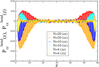
Figure 1: Contributions of the bending potential to the normal and parallel components of the pressure tensor $p_{zz}^{bend}(z),\;p_{xx}^{bend}(z)$ across a slit of width $L_{z}=60$ for chains with different length $N=4,\;10$ and $20$, monomer density $\rho=0.0625$, and bending stiffness $\epsilon_{b}/k_{B}T=100$.

II.3 Some Remarks About Our Implementation of Density Functional Theory (DFT)

In our implementation of DFT, we use a slightly different microscopic model from the one described in Section II.1. Specifically, instead of employing FENE and WCA pairwise segment-segment potentials (Eqs. (1) and (2)), we model the polymer molecule as a necklace of tangent hard spheres of diameter $\sigma$, whose degree of stiffness is governed by the bending potential given by Eq. (3).

The starting point of any DFT approach evans79 is the expression for the Helmholtz free energy as a functional of the nonuniform molecular density $\rho_{mol}(\vec{r},\omega)=\rho_{iso}(\vec{r})f(\vec{r},\omega)$, where $\rho_{iso}(\vec{r})$ is the isotropic (orientationally independent) part and $f(\vec{r},\omega)$ is the spatially- and angularly-dependent orientational distribution function. Here $\omega$ is a compact notation for the polar angles $\theta$ and $\phi$, and $f(\vec{r},\omega)$ is defined as an average over all the bonds cao06c and is normalized according to:

$$\int d\omega f(\vec{r},\omega)=\int_{0}^{2\pi}d\phi\int_{0}^{\pi}d\theta\sin\theta f(\vec{r},\theta,\phi)=1.$$ (13)

For the isotropic phase in the bulk, $f_{iso}(\omega)=1/(4\pi)$ everywhere. However, even though we will be primarily concerned with isotropic regime in the present work, due to the presence of confining flat walls, which exert an ordering effect on the polymers, $f(\vec{r},\omega)$ is expected to display a non-trivial spatial and angular variation.

In this regard, we note that there have been several earlier DFT-based studies of semiflexible polymers confined in a flat slit. forsman03 ; forsman06 ; turesson07 However, in these works only the orientationally independent molecular density $\rho_{iso}(\vec{r})$ was considered. At the same time, as will be seen below, even in the isotropic state the nontrivial orientational dependence (due to the walls) plays an important role in determining the surface tension $\gamma$. On the other hand, the existing DFT-based studies of isotropic-nematic behavior of semiflexible polymers in the bulk fynewever98 ; cao04 ; jaffer01 operate with the spatially uniform molecular density $\rho_{mol}(\vec{r},\omega)=\rho_{mol}f(\omega)$, where $\rho_{mol}$ is the molecular bulk number density.

For the present problem, where one needs to take into account both spatial and angular dependence of $\rho_{mol}(\vec{r},\omega)$, it is necessary to generalize the previously developed DFT approaches accordingly. While several DFT-based studies of hard rods vanroij00 ; cao06c and spherocylinders delasheras03 confined in a slit have been reported, no comparable method, to the best of our knowledge, has been proposed for semiflexible molecules (note, that Chen and Cui chen95b used self-consistent field theory (SCFT) to study the structure of the orientational wetting layer of semiflexible polymers in the vicinity of a hard-wall surface; however, it has been established that DFT, in general, is more accurate than SCFT in resolving fine structural details of polymers at a wall egorov10b ). Hence, the aim of the present work is to develop a method capable of treating both angular anisotropy and spatial inhomogeneity of semiflexible polymers within the DFT framework.

Quite generally, one can write the Helmholtz free energy functional as a sum of the ideal and excess terms:

$$\frac{F(\rho_{mol}(\vec{r},\omega))}{k_{B}T}=\frac{F_{id}(\rho_{mol}(\vec{r},\omega))}{k_{B}T}+\frac{F_{exc}(\rho_{mol}(\vec{r},\omega))}{k_{B}T}.$$ (14)

The ideal term is known exactly:

$$\frac{F_{id}(\rho_{mol}(\vec{r},\omega))}{k_{B}T}=\int d\vec{r}\int d\omega\rho_{mol}(\vec{r},\omega)(\ln[4\pi\rho_{mol}(\vec{r},\omega)]-1).$$ (15)

The excess term we split into “isotropic” ($F_{exc}^{iso}(\rho_{iso}(\vec{r}))$) and “orientational” ($F_{exc}^{orient}(\rho_{mol}(\vec{r},\omega))$) components. The former, which depends only on the isotropic part of the molecular density, is calculated from the Generalized Flory Dimer (GFD) theory, honnell89 as described in detail in Refs. forsman03, ; forsman06, ; turesson07, . The latter is obtained on the basis of a density expansion (around the spatially and angularly isotropic fluid) truncated at the second-order term: patra97

$$\frac{F_{exc}^{orient}(\rho_{mol}(\vec{r},\omega))}{k_{B}T} = \int d\vec{r}\int d\omega\int d\vec{r}^{\prime}\int d\omega^{\prime}a_{resc}^{PL}(\rho_{iso}(\vec{r}))(\rho_{mol}(\vec{r},\omega)-\rho_{mol}/(4\pi))$$ (16)

$$\times (V_{exc}(\vec{r},\vec{r}^{\prime},\omega,\omega^{\prime})-\langle V_{exc}^{iso}\rangle)(\rho_{mol}(\vec{r}^{\prime},\omega^{\prime})-\rho_{mol}/(4\pi)),$$

where $V_{exc}(\vec{r},\vec{r}^{\prime},\omega,\omega^{\prime})$ is the excluded volume for 2 semiflexible polymers with angular orientations $\omega$ and $\omega^{\prime}$ (from which we have subtracted its spherical average $\langle V_{exc}^{iso}\rangle$ in order to avoid the double-counting of the isotropic contribution to the excess free energy, which is already taken into account via the GFD-based term). In the above equation, $a_{resc}^{PL}(\rho_{iso}(\vec{r}))$ is the (spatially dependent delasheras03 ) Parsons-Lee parsons79 ; lee87 rescaling factor, which is given in Ref. delasheras03, . This factor is needed in order to account for the higher-order virial coefficients in this Onsager-like onsager49 expression for the excess free energy. The central quantity in Eq. (16) is the spatially- and orientationally-dependent excluded volume $V_{exc}(\vec{r},\vec{r}^{\prime},\omega,\omega^{\prime})$. While an explicit analytical expression is known for this quantity for 2 rigid rods under planar confinement, shundyak01 no comparable expression is available for 2 semiflexible molecules. Accordingly, we adopt a simple decoupling approximation and write $V_{exc}(\vec{r},\vec{r}^{\prime},\omega,\omega^{\prime})\approx\delta(\vec{r}-\vec{r}^{\prime})V_{exc}(\omega,\omega^{\prime})$, where for the angularly-dependent term $V_{exc}(\omega,\omega^{\prime})$ we use an empirical expression due to Fynewever and Yethiraj obtained by fitting the corresponding two-chain simulation data. fynewever98 The corresponding spherical average is given by $\langle V_{exc}^{iso}\rangle=\int d\omega\int d\omega^{\prime}V_{exc}(\omega,\omega^{\prime})/(16\pi^{2})$. In what follows, we will study inhomogeneous semiflexible polymer solution confined by two infinite flat hard walls located at $z=0$ and $z=L_{z}$. Accordingly, the isotropic molecular density profile is a function of $z$ only and the corresponding expression for the grand potential takes the form:

$$\Omega(\rho_{mol}(z,\omega))=F(\rho_{mol}(z,\omega))+\int_{0}^{h}dz\int d\omega\rho_{mol}(z,\omega)[V_{ext}^{mol}(z,\omega)-\mu],$$ (17)

where $\mu$ is the polymer chemical potential and $V_{ext}^{mol}(z,\omega)$ is the external potential due to the two hard walls acting on the polymer molecules.

The equilibrium distributions $\rho_{iso}(z)$ and $f(z,\omega)$ are obtained by minimizing the grand potential with respect to $\rho_{iso}(z)$ and $f(z,\omega)$, respectively lichtner12 . In practice, the minimization is performed in two steps telodagama84 . First, one minimizes $\Omega$ with respect to $\rho_{iso}(z)$ as described in detail in Refs. forsman03, ; forsman06, ; turesson07, , which yields the following result for the equilibrium isotropic distribution forsman03 ; forsman06 ; turesson07 :

$$\rho_{iso}(z) = e^{\mu/k_{B}T}\sum_{i=1}^{N}\int_{0}^{L_{z}}\delta(z-z_{i})\prod_{j=1}^{N}e^{-\lambda(z_{j})}\prod_{k=1}^{N-1}\Theta(|\Delta z_{k}|-\sigma)$$ (18)

$$\times \prod_{l=1}^{N-2}\Psi(\Delta z_{l},\Delta z_{l+1})dz_{1}\cdots dz_{N},$$

where the indices $i,j,k,l$ label individual monomers, i.e. the total density distribution is written as a sum over monomer density distributions.

In the above equation,

$$\Psi(\Delta z_{i},\Delta z_{i+1}) = \exp[\epsilon_{b}/k_{B}T(1-\Delta z_{i}\Delta z_{i+1}/\sigma^{2})]$$ (19)

$$\times I_{0}\left\{\epsilon_{b}/k_{B}T\left[1-\left(\frac{\Delta z_{i}}{\sigma}\right)^{2}\right]^{1/2}\left[1-\left(\frac{\Delta z_{i+1}}{\sigma}\right)^{2}\right]^{1/2}\right\},$$

where $I_{0}(x)=\frac{1}{2\pi}\int_{0}^{2\pi}\exp[-x\cos\phi]d\phi$ is a modified Bessel function and $\Delta z_{i}=z_{i+1}-z_{i}$. In addition, $\lambda(z)=[\delta F_{exc}^{iso}/\delta\rho_{iso}(z)+v_{ext}^{mon}(z)]/k_{B}T$, where $v_{ext}^{mon}(z)$ is the external potential due to the two hard walls acting on individual monomers, which is equal to zero for $0<z<L_{z}$ and is infinite otherwise. Finally, $\Theta(x)$ in Eq. (18) is the Heaviside step function, which is equal to unity for non-positive values of its argument and is equal to zero for $x>0$.

Given that $\rho_{iso}(z)$ in Eq. (18) is written as a sum of contributions from individual monomers, one can readily obtain the zeroth approximation to the orientational distribution function, $f_{0}(z,\omega)$, which includes the orienting effect on the polymer molecules due to the hard walls cao06c , but not due to the Onsager-like term in Eq. (16), which has not been treated yet.

As the second step in the minimization procedure, we now minimize the grand potential with respect to $f(z,\omega)$, which yields the following result for the equilibrium orientational distribution function: lichtner12 ; telodagama84

$$f(z,\omega)=C(z)\exp[-V_{eff}(z,\omega)/k_{B}T]\exp[-2a_{resc}^{PL}(\rho_{iso}(z))\int d\omega^{\prime}(\rho_{mol}(z,\omega^{\prime})-\rho_{mol}/(4\pi))(V_{exc}(\omega,\omega^{\prime})-\langle V_{exc}^{iso}\rangle)],$$ (20)

where $C(z)$ is the normalization constant ensuring that $\int d\omega f(z,\omega)=1$ for all $z$. The angular- and spatially-dependent effective external potential is given by $V_{eff}(z,\omega)=-k_{B}T\ln[f_{0}(z,\omega)]$. In practice, Eq. (20) is solved iteratively, by using $f_{0}(z,\omega)$ as the initial guess and iterating until the converged result for $f(z,\omega)$ is obtained. Note that due to the averaging over the $xy$ (hard wall) plane, the orientational distribution function $f(z,\theta)$ depends on $z$ and $\theta$ only, but not on the azimuthal angle $\phi$, which precludes the treatment of biaxiality within our spatially one-dimensional DFT approach.

Once the equilibrium orientational distribution function $\rho_{mol}(z,\theta)=\rho_{iso}(z)f(z,\theta)$ is computed, one can readily obtain the order parameter as a function of the distance from the wall:

$$S(z)=2\pi\int_{0}^{\pi}d\theta f(z,\theta)(\frac{3}{2}\cos^{2}\theta-\frac{1}{2}).$$ (21)

Recall that the orientational distribution function $f(z,\omega)$ is defined as an average over all the bonds in the molecule. cao06c From the above definition it is clear that $S(z)=0$ corresponds to random chain orientation, while $S(z)=-0.5$ corresponds to perfect alignment of the chain parallel to the wall.

In addition, various thermodynamic quantities can be calculated, including the surface tension at the wall. As follows from the above discussion, $\gamma$ contains isotropic and orientational contributions in both its ideal and excess terms. For example, for the isotropic contribution to the ideal term one gets: forsman03 ; forsman06 ; turesson07

$$\frac{\gamma_{id}^{iso}\sigma^{2}}{k_{B}T}=\int_{0}^{h}dz(\rho_{mol}-\rho_{iso}(z)),$$ (22)

and for the orientational contribution one obtains: perera88

$$\frac{\gamma_{id}^{orient}\sigma^{2}}{k_{B}T}=2\pi\int_{0}^{h}dz\int_{0}^{\pi}d\theta\rho_{mol}(z,\theta)\ln[4\pi\rho_{mol}(z,\theta)/\rho_{mol}].$$ (23)

Likewise, the expressions for the isotropic and orientational contributions to the excess part of the surface tension can be readily obtained from the corresponding parts of the excess Helmholtz free energy.

In presenting the DFT results below, we will split the total surface tension into its isotropic and orientational components: $\gamma=\gamma^{iso}+\gamma^{orient}$, where $\gamma^{iso}=\gamma^{iso}_{id}+\gamma^{iso}_{exc}$ and $\gamma^{orient}=\gamma^{orient}_{id}+\gamma^{orient}_{exc}$.

III Molecular Dynamics Results for Semiflexible Polymers at Repulsive Walls

In presenting our results in this and the following section, we make all distances dimensionless by measuring them in units of the size parameter $\sigma$ and all energies in units of the thermal energy $k_{B}T$.

In Fig. 2 we display the impact of growing chain stiffness on the distribution of monomer density across a slit with $L_{z}=40$ for a system of semiflexible polymers at concentration $\rho=0.1$ and two different chain lengths, $N=16,\;N=32$. One may detect a qualitative change in the density profiles whereby an increasingly pronounced depletion of macromolecules in the vicinity of the confining walls is observed irrespective of chain length $N$. As a consequence, the density sufficiently far away from the walls exceeds slightly yet steadily the average density in the slit with increasing rigidity, $\epsilon_{b}/k_{B}T=1,\;5,\;10,\;30$, which should be kept in mind when MD data are compared to DFT results where density corresponds to that in a grand canonical ensemble. Nonetheless, Fig. 2 manifests a very good agreement between the two methods, MD and DFT, as far as the profiles of monomer density are concerned, whereby the DFT results have been obtained for $\rho_{b}=\rho_{middle}$. When the density profile gets horizontal over an extended range of $z$ near the middle point $z_{middle}=L_{z}/2$ of the slit, the two walls are essentially independent of each other, and $\rho_{middle}$ should be equal to the bulk density of a semi-infinite system.

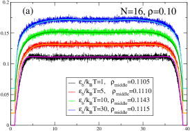
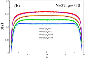
Figure 2: (a) The monomer density profiles $\rho(z)$ across the film for $L_{z}=40$ and four values of the chain stiffness parameter, $\epsilon_{b}/k_{B}T=1,5,10$ and $30$, for $N=16$ and $\rho=0.1$. Noisy lines are from MD, smooth lines from DFT (performed at the values of the bulk density $\rho_{b}$ corresponding to the MD values of $\rho_{middle}$ indicated in the legend). All profiles are shifted vertically by $0.02$ for better visibility. (b) The monomer density profiles $\rho(z)$ across the film for $L_{z}=40$ and four values of the chain stiffness parameter, $\epsilon_{b}/k_{B}T=1,\;5,\;10$ and $30$, for $N=32$ and $\rho_{b}=\rho_{middle}$. Noisy lines are from MD, smooth lines from DFT, and the profiles are shifted vertically by $0.015$.

Next we focus on the behavior of the surface tensions $\gamma_{wall}$ in the regime of densities $\rho\leq 0.1$ and not extremely stiff chains, so we stay far away from the isotropic to nematic transition (Fig. 3). At these

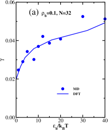
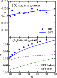
Figure 3: (a) Surface tension as a function of the chain stiffness parameter $\epsilon_{b}/k_{B}T$ for $\rho_{b}=0.1$, $N=32$, comparing MD results (dots) with DFT predictions (lines). (b) Surface tension as a function of the chain length for $\rho_{b}=0.065$ and the stiffness parameter $\epsilon_{b}/k_{B}T=16$ (upper panel) and $\epsilon_{b}/k_{B}T=100$ (lower panel), comparing MD results (dots) with DFT predictions (lines); the decomposition of the DFT result into isotropic and orientational components is shown for the stiff chain, $\epsilon_{b}/k_{B}T=100$.

low densities, accurate estimation of the osmotic pressure tensor components spatially resolved near repulsive walls is rather difficult, and hence the application of Eq. 12 suffers from rather large statistical errors. In

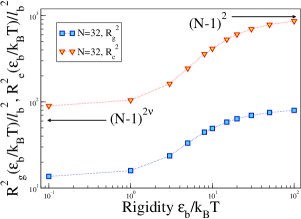
Figure 4: Mean square end-to-end distance $\langle R_{e}^{2}\rangle$ and mean square gyration $\langle R_{g}^{2}\rangle$ radius (plotted in units of the squared bond length $\ell_{b}$) vs. the rigidity parameter $\epsilon_{b}/k_{B}T$. All data were taken for a density $\rho_{b}=0.0625$ in a box of linear dimensions $40\times 40\times 40$, using periodic boundary conditions and a chain length $N=32$. Arrows denote the squared end-to-end distance $R_{e}^{2}/\ell_{b}^{2}$ in the limit of a flexible coil and a rigid rod.

Fig. 3a we present the surface tension as a function of the chain stiffness parameter $\epsilon_{b}/k_{B}T$ for $\rho_{b}=0.1$, $N=32$, comparing MD results (dots) with DFT predictions (lines). One sees that the two methods are in nearly quantitative agreement, both predicting monotonic increase of the surface tension with increasing $\epsilon_{b}/k_{B}T$. In Fig. 3b we present the surface tension as a function of the chain length for $\rho_{b}=0.065$ for two values of the stiffness parameter: $\epsilon_{b}/k_{B}T=16$ (upper panel) and $\epsilon_{b}/k_{B}T=100$ (lower panel). Once again, MD and DFT are in nearly quantitative agreement. For more flexible chain ($\epsilon_{b}/k_{B}T=16$), both methods predict that $\gamma$ increases very slowly with $N$, while for the stiffer chain ($\epsilon_{b}/k_{B}T=100$), the increase is more pronounced. For the stiffer chain, we show the decomposition of the DFT result for $\gamma$ into the isotropic and orientational terms; one sees that the orientational term becomes increasingly prominent with increasing chain length. For more flexible chain, the DFT result for $\gamma$ is dominated by the isotropic term (decomposition not shown). The smallness of the surface tension in this region of parameters is expected, of course, due to the smallness of the considered density: with increasing density the surface tension increases rather fast. Note that due to the large fluctuations of the MD data in Fig. 3 we have disregarded the distinction between the average density $\rho$ in the simulation box and the bulk density $\rho_{b}$ (which is seen only near $z\approx h/2$ and only if $L_{z}$ is chosen large enough, cf. Fig. 1).

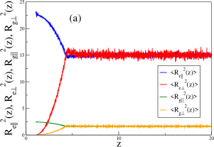
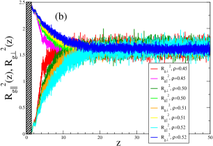
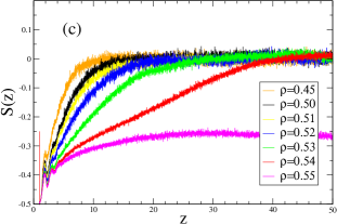
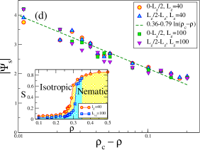
Figure 5: (a) Components of the mean square end to end distance $\langle R_{e}^{2}(z)\rangle$ and radius of gyration $\langle R^{2}_{g}(z)\rangle$, parallel $(\langle R_{e||}^{2}(z)\rangle),\langle R_{g||}^{2}(z)\rangle$ and perpendicular $(\langle R_{e\bot}^{2}(z)\rangle,\langle R_{g\bot}^{2}(z)\rangle)$ to the confining walls, plotted versus the distance $z$ of the center of mass of each polymer from the nearest wall. All data refer to $N=8$, $\epsilon_{b}/k_{B}T=100$, average density in the system being $\rho=0.1$, and $L_{z}=40$. (b) Components of the mean square gyration radius of the polymers parallel $(\langle R_{g||}^{2}(z)\rangle)$ and perpendicular $(\langle R_{g\bot}^{2}(z)\rangle)$ to the confining walls plotted as a function of distance $z$ of the center of mass of the polymer from the nearest wall. All data refer to $N=8$, $\epsilon_{b}/k_{B}T=100,L_{z}=100$, and several average densities in the simulation box are shown, as indicated in the key to the figure. (c) Mean orientation of bonds $S(z)$ [see text] plotted versus the distance $z$ of a bond from the nearest wall, for the case $N=8,\epsilon_{b}/k_{B}T=100,L_{z}=100$, and various average densities in the simulation box, as indicated in the key to the figure. (d) Surface-induced excess order parameter $|\Psi_{s}|$, where $\Psi_{s}$ is obtained as $\Psi_{s}=\int_{0}^{L_{z}/2}dzS(z)$, plotted vs the density difference $\rho_{c}-\rho$, $\rho_{c}$ being the critical density where nematic order starts to set in. Note that the results for $2$ values of $L_{z}$ are included. Estimates are extracted from the surface-induced excess order parameter at both walls and shown individually, to indicate the magnitude of statistical errors. A logarithmic abscissa scale is used to show that the data are compatible with the expected logarithmic divergence as $\rho$ approaches $\rho_{c}$. The inset displays the phase diagram (i.e., the variation of $S$ with $\rho$) for the widths $L_{z}=40,\;100$.

While the variation of $\epsilon_{b}/k_{B}T$ on the surface tension has a rather weak effect (Fig. 3), one should recall that the change in the actual conformations of the macromolecules is very pronounced (Fig. 4). Under the shown conditions one observes a crossover from self-avoiding walk-like behavior $(\langle R_{e}^{2}\rangle\propto\ell_{b}^{2}N^{2\nu})$ to rod-like behavior $(\langle R_{e}^{2}\rangle\approx\ell_{b}^{2}(N-1)^{2}$ as $\epsilon_{b}/k_{B}T$ varies from $\epsilon_{b}/k_{B}T=0$ to $\epsilon_{b}/k_{B}T=100$.

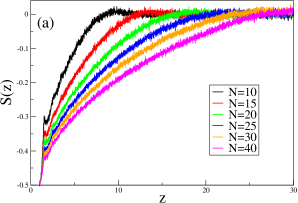
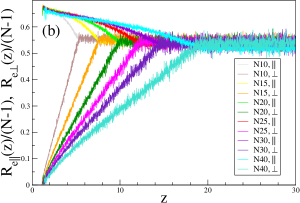
Figure 6: (a) Bond orientational order parameter $S(z)$ plotted vs. the distance $z$ from the nearest wall, as in Fig. 5c, but now for the case $\rho$=0.0625, $\epsilon_{b}/k_{B}T$=100, $L_{z}$=60, and chain lengths $N$ from $N=10$ to $N=40$, as indicated in the key to the figure. Note that $L_{x}=L_{y}=100$ and bins of thickness $\Delta z=0.01$ were chosen, to reach both good statistics and a fine enough resolution of the profile. (b) Components of the normalized end-to-end vector $(\langle R_{e\|}^{2}(z)\rangle)^{1/2}/(N-1)$, $\langle R_{e\bot}^{2}(z)\rangle^{1/2}/(N-1)$, parallel and perpendicular to the confining walls, plotted versus the distance $z$ of the center of mass of a polymer from the nearest wall. Chain lengths $N$ from $N=10$ to $N=40$ are shown, as indicated by the key. All data are for $\rho=0.0625,L_{x}=L_{y}=100$, $L_{z}=60$, and $\epsilon_{b}/k_{B}T=100$ whereby due to symmetry only the left half of the profiles is shown.

Of course, it is very interesting to study the linear dimensions of the macromolecules when they are confined by the parallel repulsive walls. Fig. 5a presents plots of the components of the mean square end-to-end distance parallel $(R_{e\|}^{2}(z))$ and perpendicular $(R_{e\bot}^{2}(z))$ to the wall, as well as the corresponding mean square gyration radii $(R_{g||}^{2}(z),R_{g\bot}^{2}(z))$, resolved as a function of distance $z$ of the center of mass of the chain, for a very short $(N=8)$ and stiff $(\epsilon_{b}/k_{B}T=100)$ polymer, at a small density $\rho=0.1$. One sees that near the walls $(z\leq 4)$ the perpendicular component is reduced and the parallel component is enhanced, indicating that the short stiff chains are rather strongly aligned parallel to the walls. The bulk value $R^{2}_{ez}=R_{\ell||}^{2}\approx 15$ is only slightly smaller than the theoretical value for a rigid rod containing $N=8$ beads connected by links of length $\ell_{b}\approx 0.96,L^{2}/3=15.05$, and the value $R_{\ell||}^{2}\approx 22.5$ is consistent with the expected value $L^{2}/2$ for rigid rods of length $L=6.72$. For these stiff short chains the bulk ratio $R_{e}^{2}/R_{g}^{2}\approx 10$ still falls below its limit (12) reached for long rods $N\rightarrow\infty$, as expected.

Closer to the transition isotropic/nematic in the bulk (Fig. 5b), the orienting effect of the wall on the short stiff chains extends much further than half their length, and reflects the formation of the wall-induced nematic layer, which can also be seen from the mean orientation of bonds (Fig. 5c), as measured by the second Legendre polynomial $S(z)=P_{2,z}(\cos\theta)=[3\langle\cos^{2}\theta\rangle-1]/2$, $\theta$ being the angle with respect to the $z$-axis, normal to the confining walls. Recall that $S(z)=-0.5$ means perfect alignment parallel to the walls. In Fig. 5c, the $z$-coordinate of a bond between monomers $i$ and $i+1$ ($i$ being an index labeling the monomers along the considered chain) is simply defined as $z=(z_{i}+z_{i+1})/2$, and the angular brackets $\langle\cdot\rangle$ denote an average over all the bonds of all the chains that fall in an interval $[z-0.01,z+0.01]$. Since in isotropic phase in the bulk the order parameter $S$ is equal to zero, one can define the surface-induced excess order parameter as follows: $\Psi_{s}=\int_{0}^{L_{z}/2}dzS(z)$; the corresponding results are presented in Fig. 5d.

When the density $\rho$ of the effective monomers increases up to the critical density $\rho_{c}$ where nematic order starts to occur in the bulk, a surface-induced nematically ordered layer forms at the repulsive wall. Fig. 5d shows that the thickness of this nematic surface layer diverges logarithmically towards infinity when $\rho$ tends towards $\rho_{c}$. A related surface-induced ordering has already been found for a lattice model ivanov13 ; ivanov14 .

Of course, it is also interesting to ask what changes when the length of the polymers is varied. Fig. 6a shows that even at a low average density $\rho$ in the simulation box (recall that $\rho$ slightly differs from $\rho_{b}$, as pointed out in the discussion of Fig. 1), the range over which the wall leads to predominantly parallel bond orientation increases substantially, as $N$ increases. Note that for $\rho=0.0625$ and $N\geq 30$ there is no longer a well-defined extended bulk region of the isotropic phase (where $P_{2}(\cos\theta)=0$) for $L_{z}=60$. This is not evident from the components of the end-to-end vector, however (Fig. 6b). There the range over which the wall strongly matters always seems to be simply $z\approx(N-1)\ell_{b}/2$. But although for $N=40$ the components parallel and perpendicular to the wall reach horizontal plateaus in the center, the fact that these plateaus differ also is a clear evidence that there is no longer any bulk region in the system. Note that despite the low density the behavior observed in Fig. 6 is very different from wall effects on a dilute solution of flexible polymers (which would behave like self-avoiding walks under good solvent conditions), but rather chains here are like slightly flexible rods, for the chosen parameters.

IV DFT Results for Semiflexible Polymers at Repulsive Walls

IV.1 The effect of varying chain stiffness

We begin by considering the effect of varying the chain stiffness parameter on the density profiles, bond orientational order parameter, and the surface

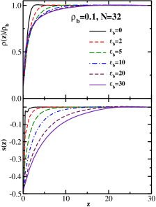
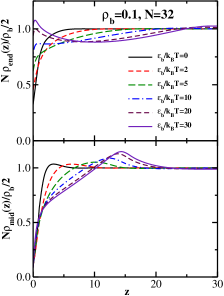
Figure 7: (a) Upper panel: the normalized monomer density profiles $\rho(z)/\rho_{b}$ for six values of the chain stiffness parameter: $\epsilon_{b}/k_{B}T=$0, 2, 5, 10, 20, and 30; $N$=32 and $\rho_{b}$=0.1. Lower panel: same for the bond orientational order parameter $S(z)$. (b) Upper panel: the normalized end-monomer density profiles for six values of the chain stiffness parameter: $\epsilon_{b}/k_{B}T$=0, 2, 5, 10, 20, and 30; $N$=32 and $\rho_{b}$=0.1. Lower panel: same for the two middle monomers (segments number 16 and 17).

tension. We set the chain length to $N$=32 and the bulk monomer density to $\rho_{b}$=0.1. The DFT results for the total monomer density profiles (normalized by the bulk monomer density) are shown in the upper panel of Fig. 7a for several values of the chain stiffness parameter $\epsilon_{b}/k_{B}T$. As one would expect, the range of the depletion zone grows with increasing $\epsilon_{b}/k_{B}T$, which leads to increasing surface tension as was already seen in Fig. 3. In the lower panel of Fig. 7a we show DFT results for the bond orientational order parameter $S(z)$ defined by Eq. (21). One sees that with increasing chain stiffness the tendency of the chains to be aligned parallel to the wall extends to larger distances from the wall. Returning to the monomer density profiles displayed in the upper panel of Fig. 7b, one observes an (almost imperceptible) maximum in these profiles beyond the depletion zone. The same phenomenon has been reported in an earlier study of fully flexible chains, where the appearance of this maximum was related to the segregation of end-monomers to the wall. shvets13

Accordingly, it is of interest to consider the effect of the chain stiffness on the end-monomer density distributions. Indeed, the enrichment of chain ends at surfaces and interfaces has been studied for a long time in polymer melts wang91c ; matsen14 , while dilute polymer solutions have received little attention in this regard. In the upper panel of Fig. 7b, we display the DFT results for the end-monomer density profiles $\rho_{end}(z)$ (normalized by their bulk values). One immediately sees that the contact value $\rho_{end}(0)$ grows dramatically with increasing $\epsilon_{b}/k_{B}T$. By contrast, the contact value of the total monomer density $\rho(0)$ (see upper panel of Fig. 7a) is essentially $\epsilon_{b}/k_{B}T$-independent. Accordingly, the ratio $\rho_{end}(0)/\rho(0)$ is expected to be a strongly increasing function of $\epsilon_{b}/k_{B}T$. This is indeed confirmed in Fig. 8a where we plot the ratio of the end-monomer to the total density profile defined by: wang91c

$$\phi_{e}(z)=\frac{N}{2}\frac{\rho_{end}(z)}{\rho(z)}$$ (24)

One sees that in the vicinity of the wall the end-monomer density is always enhanced relative to the total density (and the degree of this enrichment grows with $\epsilon_{b}/k_{B}T$), while away from the wall there is concomitant depletion (as the difference between the two normalized profiles must integrate to 0 over the entire slit). It is also worth pointing out that the absolute values of this enrichment at the wall are significantly greater compared to the case of polymer melt. wang91c Note also that the enrichment of chain ends at the walls is pronounced in a very narrow region (of width $\Delta z<\sigma$), while the corresponding adjacent depletion zone is spread out over a much broader region (of width $\Delta z\gg\sigma$), and hence is difficult to recognize visually in Figs. 8 and 9. At this point we recall that MD simulations are performed in the canonical ensemble at the average density $\rho$, while DFT calculations are performed in the grand-canonical ensemble at the bulk density $\rho_{b}$. Due to the depletion of the density near the walls in a slit of finite width, such as used in MD simulations, it is a nontrivial task (subject to both statistical and systematic errors) to convert the average density $\rho$ in MD to the corresponding bulk density $\rho_{b}$, although for the cases shown here we expect that $\rho$ and $\rho_{b}$ differ only slightly.

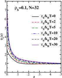
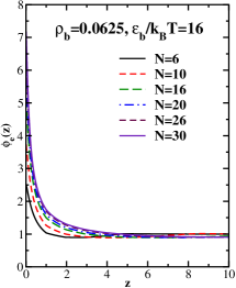
Figure 8: (a) The ratio of the end-monomer to the total density profile for six values of the chain stiffness parameter: $\epsilon_{b}/k_{B}T=$0, 2, 5, 10, 20, and 30; $N=32$, and $\rho_{b}$=0.1. (b) The ratio of the end-monomer to the total density profile for six values of the chain length: $N$=6, 10, 16, 20, 26, and 30; $\epsilon_{b}/k_{B}T$=16 and $\rho_{b}$=0.0625.

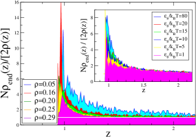
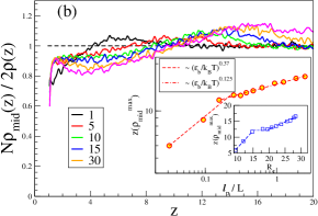
Figure 9: (a) MD results for the normalized density of end-monomers in the vicinity of a wall for $N=32,\;\epsilon_{b}/k_{B}T=32$ vs $z$ for different total monomer concentration $\rho$ and $L_{z}=100$. Inset shows $N\rho_{end}(z)/[2\rho(z)]$ against $z$ for several values of the chain stiffness $\epsilon_{b}/k_{B}T$ and $L_{z}=40$. (b) MD results for the normalized density of mid-monomers for $N=$32, $\rho_{b}$ = 0.1 vs $z$ for several values of the chain stiffness $\epsilon_{b}/k_{B}T$ as indicated in the legend. Inset shows the location of the maximum vs $\ell_{p}/L$; the inset of the inset shows the location of the maximum vs $R_{e}$.

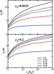
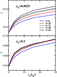
Figure 10: (a) Upper panel: The DFT results for the contact value $\phi_{e}(0)$ as a function of the chain stiffness for six values of the chain length: $N$=6, 8, 12, 16, 24, and 32; $\rho_{b}$=0.065. Lower panel: same for $\rho_{b}$=0.2. (b) Upper panel: The DFT results for the surface tension as a function of the chain stiffness for six values of the chain length: $N$=6, 8, 12, 16, 24, and 32; $\rho_{b}$=0.065. Lower panel: same for $\rho_{b}$=0.2.

Given that the end-monomers are segregated to the wall and depleted away from the wall, one would expect the opposite to hold for the middle monomers. This is confirmed in the lower panel of Fig. 7b, which shows the DFT results for the normalized middle-monomer density profiles (segments number $i$=16 and 17 for $N$=32). There is indeed a noticeable enhancement of the middle-monomer density away from the wall, which increases with the chain stiffness. This enhancement helps to explain the weak maximum observed in $\rho(z)$ in Fig. 7a away from the depletion zone. In order to confirm the above DFT predictions regarding the spatial distributions of end- and mid-monomers, we present in Fig. 9 the corresponding MD results, which all show the same trends as the DFT data. Of course, in MD work the price that one has to pay in order to have a very fine spatial resolution in $z$ are significant statistical fluctuations, which are absent in DFT.

All the DFT results reported so far were limited to one particular chain length ($N$=32) and a single value of the monomer bulk density ($\rho_{b}$=0.1). One major advantage of the DFT approach is its computational efficiency, which allows a relatively fast exploration of the parameter space (furthermore, the accuracy of the present DFT approach has been confirmed via comparisons with the corresponding MD results). In order to exploit this advantage, we present in Fig. 10a the DFT results for the contact value $\phi_{e}(0)$ as a function of the chain stiffness for six values of the chain length: $N$=6, 8, 12, 16, 24, and 32. The upper panel displays the results for the bulk monomer density $\rho_{b}=0.065$, while the lower panel gives the results for $\rho_{b}=0.2$. One sees that the segregation of the chain ends to the surface increases monotonocally with the chain stiffness for all the chain lengths considered. For a given value of $\epsilon_{b}/k_{B}T$, the segregation increases with increasing chain length and with decreasing bulk density.

In Fig. 10b, we present a similar set of the DFT results for the surface tension as a function of $\epsilon_{b}/k_{B}T$ for six values of the chain length and two values of the bulk monomer density. Similar to the behavior of $\phi_{e}(0)$, $\gamma$ increases monotonically with $\epsilon_{b}/k_{B}T$ for all the values of $N$ and $\rho_{b}$. For a given value of $\epsilon_{b}/k_{B}T$, the surface tension increases with the chain length for stiffer chains ($\epsilon_{b}/k_{B}T\geq 2$), while for more flexible chains, the opposite trend is observed.

IV.2 The effect of varying chain length

Next, we consider the effect of varying chain length at a fixed value of the stiffness parameter. The DFT results for the total monomer density profiles (normalized by the bulk monomer density) are shown in the upper panel of

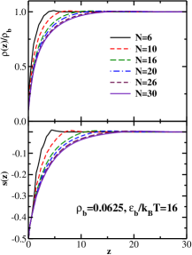
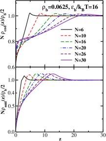
Figure 11: (a) Upper panel: the normalized monomer density profiles $\rho(z)/\rho_{b}$ for six values of the chain length: $N$=6, 10, 16, 20, 26, and 30; $\epsilon_{b}/k_{B}T$=16 and $\rho_{b}$=0.0625. Lower panel: same for the bond orientational order parameter $S(z)$. (b) Upper panel: the normalized end-monomer density profiles for six values of the chain length: $N$=6, 10, 16, 20, 26, and 30; $\epsilon_{b}/k_{B}T$=16 and $\rho_{b}$=0.0625. Lower panel: same for the two middle monomers.

Fig. 11a for several values of the chain length, for $\epsilon_{b}/k_{B}T$=16 and $\rho_{b}$=0.0625. As one would expect, the range of the depletion zone grows with increasing chain length, which leads to increasing surface tension. In the lower panel of Fig. 11a we show DFT results for the bond orientational order parameter $S(z)$. One sees that with increasing chain length the tendency of the chains to be aligned parallel to the wall extends to larger distances from the wall.

Moving next to the density profiles of individual monomers, in the upper panel of Fig. 11b we display the DFT results for the end-monomer density profiles $\rho_{end}(z)$ (normalized by their bulk values), while the lower panel shows the corresponding middle-monomer profiles. Once again, the segregation of the chain ends to the wall and the enhancement of the middle-monomer density away from the wall is quite evident. Fig. 8b plots the ratio $\phi_{e}(z)$ for several values of the chain length, and one observes that the contact value $\phi_{e}(0)$ grows strongly with increasing $N$ (note that the contact value of the total monomer density $\rho(0)$, i.e. the bulk pressure, decreases with $N$). To illustrate this behavior for other values of the stiffness parameter, Fig. 12a displays the DFT results for the contact value $\phi_{e}(0)$ as a function of the chain length for nine values of the chain stiffness: $\epsilon_{b}/k_{B}T$=0, 1, 2, 3, 5, 8, 16, 24, and 32; the upper panel is for the monomer bulk density $\rho_{b}$=0.0625, while the lower panel is for $\rho_{b}$=0.2. One sees that the segregation of the chain ends to the surface increases steadily with the chain length for all the values of $\epsilon_{b}/k_{B}T$ considered. For a given value of $N$, the segregation increases with increasing chain stiffness and with decreasing bulk density.

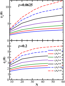
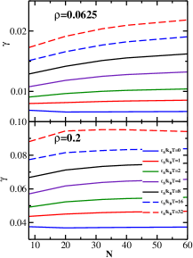
Figure 12: (a) Upper panel: The DFT results for the contact value $\phi_{e}(0)$ as a function of the chain length for nine values of the chain stiffness: $\epsilon_{b}/k_{B}T$=0, 1, 2, 3, 5, 8, 16, 24, and 32; $\rho_{b}$=0.0625. Lower panel: same for $\rho_{b}$=0.2. (b) Upper panel: The DFT results for the surface tension as a function of the chain length for nine values of the chain stiffness: $\epsilon_{b}/k_{B}T$=0, 1, 2, 3, 5, 8, 16, 24, and 32; $\rho_{b}$=0.0625. Lower panel: same for $\rho_{b}$=0.2.

In Fig. 12b, we present a similar set of the DFT results for the surface tension as a function of $N$ for nine values of the chain stiffness and two values of the bulk monomer density. For the two smallest values of $\epsilon_{b}/k_{B}T$ ($\epsilon_{b}/k_{B}T$=0 and 1), the surface tension is seen to decrease with the chain length, while for stiffer chains, the opposite behavior is observed.

V Conclusions

In this paper, a comprehensive investigation of semiflexible polymers in a solution under good solvent conditions interacting with a repulsive flat wall have been presented, combining results from extensive MD simulations with a newly extended formulation of DFT. This new formulation was required in order to take into account that both the spatial density distribution is inhomogeneous ($\rho(z)$ depends on the distance $z$ from the wall), and the angular distribution $f(z,\omega)$ of the orientation of the bonds is both spatially-dependent and anisotropic, unlike the bulk isotropic solution, where $\rho(z)=\rho_{b}$ is the given bulk density, and $f(z,\omega)=1/(4\pi)$ is also a constant everywhere.

While these wall-induced inhomogeneities of $\rho(z)$ and $f(\Omega)$ mentioned above already occur in a solution of rigid rods (at densities $\rho$ less than the density $\rho_{i}$ where in the bulk the two-phase coexistence region between isotropic (I) and nematic (N) phases begins), and it is of interest to study the range over which these wall-induced inhomogeneities extend and to clarify their interplay mao97 , in a solution of semiflexible polymers additional phenomena occur: the end-to-end vector of a chain is oriented parallel to the wall when the center of mass of the chain is close to the wall. Related to this, nontrivial profiles $R_{g||}^{2}(z),\;R_{g\bot}^{2}(z)$ of the parallel and perpendicular parts of the mean-square gyration radius of the chains occur (here $z$ means the distance of the chain center of mass from the wall). Also, chain ends get enriched (and the density of middle monomers depleted) at the wall, if the chain has its center of mass close to the wall. All these phenomena are carefully quantified in our study. Also, the surface tension of the polymer solution due to the repulsive wall is computed.

The MD simulations have utilized the standard Kremer-Grest bead-spring model, augmented by a bond bending potential (Eq. 3). The bond bending potential parameter $\epsilon_{b}/k_{B}T$ (which is basically the ratio of the persistence length $\ell_{p}$ and the bond length $\ell_{b}$) was varied from $\epsilon_{b}/k_{B}T=0$ (flexible chains, where $\ell_{p}\approx\ell_{b}$) to $\epsilon_{b}/k_{B}T=\ell_{p}/\ell_{b}=100$. If the chains are sufficiently stiff ($\epsilon_{b}/k_{B}T\geq 8$), nematic order sets in at sufficiently high monomer concentrations (since no explicit solvent was included, $\rho$ is nothing but the monomer density in the simulated system). We have checked where this onset of the nematic order occurs (see e.g. Fig. 2). While for short chains ($N\leq 16$) this happens only for rather concentrated solutions even if $\epsilon_{b}/k_{B}T$ is very large, for long chains (e.g. $N=64$) the nematic order sets in at rather small values of $\rho$ already in the bulk. In the present paper, we have deliberately avoided such densities in our simulation geometry (which is a slit with two equivalent repulsive wall a distance $L_{z}$ apart, see Fig. 1), – a study of capillary nematization for variable slit widths $L_{z}$ is planned for a subsequent study.

For dilute solutions, the surface tension due to the walls is very small (Figs. 3, 10b, and 12b), but increases both with $\epsilon_{b}/k_{B}T$ and with chain length $N$ (in the latter case, except for very flexible chains). We established a reasonably good agreement between MD and DFT (note that the statistical accuracy of MD is a problem when the surface tension is very small), while the agreement for the density profiles is nearly perfect (Fig. 2). In addition, MD confirms the DFT prediction regarding the enrichment of the end-monomers at the repulsive wall and its increase with increasing chain stiffness. All these observations give us confidence in the accuracy of the DFT approach.

The one-dimensional version of the DFT employed here cannot yield any information on the chain conformations as a whole, but this information is readily extracted from MD. Already in the bulk a gradual crossover from coils to (flexible) rods is encountered with increasing $\epsilon_{b}/k_{B}T$ (Fig. 5). At the wall, one not only observes chain orientation parallel to the wall, as mentioned above (Fig. 6a,b), but also the individual bonds of stiff chains get progressively oriented parallel to the wall, when the density increases (Fig. 6c). This surface-induced nematic ordering leads to a logarithmic growth of the thickness of the surface-induced liquid crystalline layer at the surface as $\rho$ tends toward $\rho_{i}$ where in the bulk the ordering would set in. With increasing chain length, for stiff chains the thickness of the region that is affected by the wall gets influenced over a rather wide regime (Fig. 7) even if the density is very small. This is reminiscent of the behavior of rigid rods near a wall (which are affected in their orientation over a distance equivalent to the rod length mao97 ).

The DFT calculations corroborate these findings, showing that both the density and bond orientation are affected over a distance of the order of the persistence length, even if the density is small (Fig. 7a). Interesting nonmonotonic density profiles for both end-monomers and middle-monomers are predicted when the persistence length is rather large and comparable to the contour length (Fig. 7b). While MD and DFT approaches yield qualitatively similar behavior for all the observables considered in this work, we note that an explicit quantitative between MD and DFT results for structural properties of the chains makes little sense since the chain models differ slightly (bead-spring model in MD vs tangent hard-sphere model in DFT) and also the wall potentials differ. Even for the same chain length $N$ and the same choice of $\epsilon_{b}/k_{B}T$, properties like $S(z)$, distributions of end-monomers or middle monomers must be slightly but systematically different. In view of the above, we present MD and DFT results side-by-side in order to demonstrate that the generic behavior is the same, irrespective of the precise choice of the model.

Finally, it is interesting to note that the (suitably scaled) contact value $\phi_{e}(0)$ of the end-monomer volume fraction at the wall and the surface tension have rather similar trends as functions of $\epsilon_{b}/k_{B}T$ and $N$ in the dilute regime (Figs. 10 and 12). The extended range over which stiff polymers “feel” the effect of a surface even in a dilute solution can be expected to have interesting consequences for the interaction of biopolymers (which are often rather stiff, e.g. DNA, actin etc) with biological membranes. Even more interesting phenomena might be expected if the entropic repulsion of the stiff polymers due to the wall competes with a short-range attraction, and a possible adsorption transition of the semiflexible polymers occurs forsman06 ; turesson07 ; birshtein79 ; hsu13 . We hope to address such issues in our future work.

VI Acknowledgements

S.A.E. acknowledges financial support from the Alexander von Humboldt Foundation. A.M. thanks for partial support under the grant No $BI314/24$. Parts of this research were conducted using the supercomputer Mogon and/or advisory services offered by Johannes Gutenberg University Mainz (www.hpc.uni-mainz.de), which is a member of the AHRP and the Gauss Alliance e.V. The authors gratefully acknowledge the computing time granted on the supercomputer Mogon at Johannes Gutenberg University Mainz (www.hpc.uni-mainz.de).

References

- (1) P. J. Flory, Statistical mechanics of chain molecules (Wiley: New York 1969).
- (2) P. G. de Gennes, Scaling Concepts in Polymer Physics (Cornell University Press: Ithaca 1979).
- (3) A. Y. Grosberg and A. R. Khokhlov, Statistical Physics of Macromolecules (AIP Press: Woodbury 1994).
- (4) H.-P. Hsu, W. Paul, and K. Binder, Macromolecules 43, 3094 (2010).
- (5) C. Bustamante, J. F. Marko, E. D. Siggia, and S. Smith, Science 265, 1599 (1994).
- (6) D. A. D. Parry and E. N. Baker, Rep. Prog. Phys. 47, 1133 (1984).
- (7) L. Onsager, Ann. N. Y. Acad. Sci. 51, 627 (1949).
- (8) P. G. de Gennes and J. Prost, The Physics of Liquid Crystals, 2nd ed. (Clarendon: Oxford 1992).
- (9) A. R. Khokhlov and A. N. Semenov, Physica A 108, 546 (1981).
- (10) A. R. Khokhlov and A. N. Semenov, Physica A 112, 605 (1982).
- (11) A. N. Semenov and A. R. Khokhlov, Sov. Phys. Usp. 31, 988 (1988).
- (12) M. R. Wilson and M. P. Allen, Mol. Phys. 80, 277 (1993).
- (13) A. Ciferri (ed.), Liquid Crystallinity in Polymers: Principles and Fundamental Properties (VCH Publishers: New York 1983).
- (14) M. Grell, D. D. C. Bradley, M. Inbosekarian, and E. P. Woo, Adv. Mater. 9, 798 (1997).
- (15) X. Wang, J. Engel, and C. Liu, J. Micromech. Microeng. 13, 628 (2009).
- (16) A. M. Donald, A. H. Windle, and S. Hanna, Liquid Crystalline Polymers (Cambridge University Press: Cambridge 2006).
- (17) S. J. Woltman, G. D. Jay, and G. P. Crawford, Nat. Mater. 6, 929 (2007).
- (18) A. Yethiraj, J. Chem. Phys. 101, 2489 (1994).
- (19) Z. Y. Chen and S.-M. Cui, Phys. Rev. E 52, 3876 (1995).
- (20) F. A. Escobedo and J. J. dePablo, J. Chem. Phys. 106, 9858 (1997).
- (21) D. Micheletti, L. Muccioli, R. Berardi, M. Ricci, and C. Zannoni, J. Chem. Phys. 123, 224705 (2005).
- (22) J. Z. Y. Chen, D. E. Sullivan, and X. Yuan, Europhys. Lett. 72, 89 (2005).
- (23) J. Z. Y. Chen, D. E. Sullivan, and X. Yuan, Macromolecules 40, 1187 (2007).
- (24) M. Turesson, J. Forsman, and T. Akesson, Phys. Rev. E 76, 021801 (2007).
- (25) V. A. Ivanov, A. S. Rodionova, J. A. Martemyanova, M. R. Stukan, M. Müller, W. Paul, and K. Binder, J. Chem. Phys. 138, 234903 (2013).
- (26) V. A. Ivanov, A. S. Rodionova, J. A. Martemyanova, M. R. Stukan, M. Müller, W. Paul, and K. Binder, Macromolecules 47, 1206 (2014).
- (27) W. Zhang, E. D. Gomez, and S. T. Milner, Macromolecules 48, 1454 (2015).
- (28) M. P. Allen and D. J. Tildesley, Computer Simulation of Liquids (Clarendon: Oxford 1989).
- (29) D. C. Rapaport, The Art of Molecular Dynamics Simulation, 2nd ed. (Cambridge Univ. Press: Cambridge 2004).
- (30) S. A. Egorov, A. Milchev, P. Virnau, and K. Binder, xx xx, to be submitted (2016).
- (31) G. S. Grest and K. Kremer, Phys. Rev. A 33, 3628 (1986).
- (32) K. Kremer and G. S. Grest, J. Chem. Phys. 92, 5057 (1990).
- (33) J. D. Weeks, D. Chandler, and H. C. Andersen, J. Chem. Phys. 54, 5237 (1971).
- (34) L. Schäfer, A. Ostendorf, and J. Hager, J. Phys. A. Math. Gen. 32, 7875 (1999).
- (35) J. C. Le Guillou and J. Zinn-Justin, Phys. Rev. B 21, 3976 (1980).
- (36) H.-P. Hsu and K. Binder, J. Chem. Phys. 136, 024901 (2012).
- (37) D. Shirvanyants, S. Panyukov, Q. Liao, and M. Rubinstein, Macromolecules 41, 1475 (2008).
- (38) J. P. Wittmer, H. Meyer, J. Baschnagel, A. Johner, S. Obukhov, L. Mattioni, M. Müller, and A. N Semenov, Phys. Rev. Lett. 93, 147801 (2004).
- (39) O. Kratky and G. Porod, Recl. Trav. Chim. 68, 1106 (1949).
- (40) S. A. Egorov, H.-P. Hsu, A. Milchev, and K. Binder, Soft Matter 11, 2604 (2015).
- (41) A. Milchev, J. Chem. Phys. 143, 064701 (2015).
- (42) J. Anderson, C. Lorenz, and A. Travesset, J. Comput. Phys. 227, 5342 (2008).
- (43) J. Glaser, T. D. Nguyen, J. A. Anderson, P. Liu, F. Spiga, J. A. Millan, D. C. Morse, and S. C. Glotzer, Comp. Phys. Comm. 192, 97 (2015).
- (44) J. H. Irving and J. G. Kirkwood, J. Chem. Phys. 18, 817 (1950).
- (45) J. S. Rowlinson and B. Widom, Molecular Theory of Capillarity (Clarendon: Oxford 1982).
- (46) B. D. Todd, D. J. Evans, and P. J. Daivis, Phys. Rev. E 52, 1627 (1995).
- (47) R. Evans, Adv. Phys. 28, 143 (1979).
- (48) D. P. Cao, M. H. Zhu, and W. C. Wang, J. Phys. Chem. B 110, 21882 (2006).
- (49) J. Forsman, C. E. Woodward, and B. C. Freasier, J. Chem. Phys. 118, 7672 (2003).
- (50) J. Forsman and C. E. Woodward, Macromolecules 39, 1269 (2006).
- (51) H. Fynewever and A. Yethiraj, J. Chem. Phys. 108, 1636 (1998).
- (52) D. Cao and J. Wu, J. Chem. Phys. 121, 4210 (2004).
- (53) K. M. Jaffer, S. B. Opps, D. E. Sullivan, B. G. Nickel, and L. Mederos, J. Chem. Phys. 114, 3314 (2001).
- (54) R. van Roij, M. Dijkstra, and R. Evans, J. Chem. Phys. 113, 7689 (2000).
- (55) D. de las Heras, L. Mederos, and E. Velasco, Phys. Rev. E 68, 031709 (2003).
- (56) A. Milchev, S. A. Egorov, and K. Binder, J. Chem. Phys. 132, 184905 (2010).
- (57) K. G. Honnell and C. K. Hall, J. Chem. Phys. 90, 1841 (1989).
- (58) C. N. Patra and S. K. Ghosh, J. Chem. Phys. 106, 2752 (1997).
- (59) J. D. Parsons, Phys. Rev. A 19, 1225 (1979).
- (60) S. D. Lee, J. Chem. Phys. 87, 4972 (1987).
- (61) K. Shundyak and R. van Roij, J. Phys. Cond. Matt. 13, 4789 (2001).
- (62) K. Lichtner, A. J. Archer, and S. H. L. Klapp, J. Chem. Phys. 136, 024502 (2012).
- (63) M. M. Telo da Gama, Mol. Phys. 52, 585 (1984).
- (64) A. Perera, G. N. Patey, and J. J. Weis, J. Chem. Phys. 89, 6941 (1988).
- (65) A. A. Shvets and A. N. Semenov, J. Chem. Phys. 139, 054905 (2013).
- (66) J.-S. Wang and K. Binder, J. Phys. I 1, 1583 (1991).
- (67) M. W. Matsen and P. Mahmoudi, Eur. Phys. J. E 37, 78 (2014).
- (68) Y. Mao, P. Bladdon, H. N. W. Lekkerkerker, and M. E. Cates, Mol. Phys. 92, 151 (1997).
- (69) T. M. Birshtein, E. B. Zhulina, and A. M. Skvortsov, Biopolymers 18, 1171 (1979).
- (70) H.-P. Hsu and K. Binder, Macromolecules 46, 2496 (2013).