Dynamics of energy transport and entropy production in ac-driven quantum electron systems
María Florencia Ludovico
Departamento de Física, FCEyN, Universidad de Buenos Aires and IFIBA, Pabellón I, Ciudad Universitaria, 1428 CABA Argentina
International Center for Advanced Studies, UNSAM, Campus Miguelete, 25 de Mayo y Francia, 1650 Buenos Aires, Argentina
Michael Moskalets
Department of Metal and Semiconductor Physics,
NTU ”Kharkiv Polytechnic Institute”, 61002 Kharkiv, Ukraine
David Sánchez
Instituto de Física Interdisciplinar y Sistemas Complejos
IFISC (UIB-CSIC), E-07122 Palma de Mallorca, Spain
Liliana Arrachea
Departamento de Física, FCEyN, Universidad de Buenos Aires and IFIBA, Pabellón I, Ciudad Universitaria, 1428 CABA Argentina
International Center for Advanced Studies, UNSAM, Campus Miguelete, 25 de Mayo y Francia, 1650 Buenos Aires, Argentina
Abstract
We analyze the time-resolved energy transport and the entropy production in ac-driven quantum coherent electron systems coupled to multiple reservoirs at finite temperature.
At slow driving we formulate the first and second laws of thermodynamics valid at each instant of time.
We identify heat fluxes flowing through the different pieces of the device and emphasize the importance of the energy stored in the contact and central regions for the second law of thermodynamics to be instantaneously satisfied.
In addition, we discuss conservative and dissipative contributions to the heat flux and to the entropy production as a function of time. We illustrate these ideas with a simple model corresponding to a driven level coupled to two reservoirs with different chemical potentials.
pacs:
73.23.-b, 72.10.Bg, 73.63.Kv, 44.10.+i
I Introduction
The understanding of the energy transfer in non-equilibrium open quantum systems is a fundamental problem in physics. The separation of energy in heat and useful work and dissipation is the key for a thermodynamical description. In quantum systems under ac driving, the identification of these different components of energy is a non-trivial task which is paramount to cold atoms cold ,
nanomechanical nanomec1 ; nanomec2 ,
nanoscale optoelectronical Michelini:2016ju ,
and mesoscopic electron physics elec1 ; elec2 ; wu09 ; elec3 ; elec4 ; Carrega:2015dh ; Chen:2015hu ; camp:2015 ; thermolud ; Proesmans:2016tq ; Dare:2016jk ; Bruch:2015ux .
Typically, the central piece of these systems contains a small number of particles and are driven out of equilibrium, which renders a usual thermodynamical description unreliable. However they are in contact to one or more macroscopic reservoirs with well defined thermodynamical intensive parameters.
In the recent years, the name ”quantum thermodynamics” has been coined to identify the area of Physics devoted to the study of this type of systems, which is an intersection of solid state and statistical physics. The foundations of this area were in part developed after the proposal of the Jarzynski’s equality jar
and
Crook’s theorem crook and a subsequent number of fluctuations relations fluc1 ; fluc2 ; sai08 ; for08 ; san09 ; fluc3 ; fluc4 ; nak10 ; fluc5 ; lop12 ; wan13 ; uts14 . Recently, linear response proposals in close relation to thermodynamics have been formulated for open quantum systems and quasi-classical systems under periodic driving thermolud ; thermo1 ; thermo2 ; thermo3 . The proper definition of the heat exchange between a quantum driven system and its
macroscopic environment
has been recently addressed
in the context of few-level or spin systems in contact to phononic baths heat1 ; heat2 ; heat3 and in systems of coupled quantum harmonic oscillators heat4 ; heat5 ; heat6 .
The first law of thermodynamics, being basically the conservation of the energy, is equally valid for non-equilibrium and equilibrium phenomena.
We have recently considered a model containing the minimal ingredients to address the problem of time-resolved heat transport us . It consists of a localized level under ac driving coupled to a single electron reservoir.
We have focused on slow driving and zero temperature.
By slow we mean a regime where the typical dwell time for the electrons inside the driven structure is much smaller than the driving period.
Even in such a simple setup a nontrivial effect manifests itself when the heat flow is analyzed as a function of time. Namely, the coupling region between the different parts of the system behaves like an energy reactance.
In this way, the coupling not only provides a necessary mechanism for particle and energy exchange but also contributes to the energy balance.
This contribution is of ac nature. It allows for a temporary energy storage which vanishes when averaged over time.
Our goal now is to analyze the time-resolved energy redistribution and entropy production in ac-driven quantum coherent electron systems coupled to multiple reservoirs and finite
temperature.
We show that the definition of the heat current flowing into the reservoirs presented in Ref. us is also suitable for multi-terminal devices. More interestingly, we study the behavior of the different components of the heat.
We identify conservative and dissipative contributions to a heat flux and to the entropy production as a function of time.
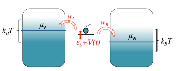
We illustrate these ideas with a simple system that consists of a slowly driven resonant level coupled to two electron reservoirs at a finite temperature and with an applied bias voltage, see Fig. 1.
Figure 1: A single electronic level is coupled to two reservoirs (fermionic baths) kept at the same temperature . The chemical potentials of the left and right reservoirs are and , respectively. The electronic level slowly evolves in time with a periodic parameter , and hence after a completed period the central part of the systems returns to its initial state.
The paper is organized as follows. We present the model in Sec. II. A thermodynamic approach to the case of slight departures from equilibrium is presented in Sec. III. Section IV contains the definition of the time-dependent energy fluxes, conservation laws and the different contributions to the entropy production. In Sec. V we focus our analysis on the slow driving regime. These ideas are then illustrated in Sec. VI, where the example of a single driven level coupled to reservoirs is analyzed in detail. Section VII is devoted to the summary and conclusions.
II Model
We consider a finite quantum system, as for example a single quantum dot or an array of quantum dots, which is driven out of equilibrium by time-periodic adiabatic power sources and in contact to several fermionic baths.
Then,
the Hamiltonian of the full system can be separated into three contributions,
(1)
The Hamiltonian representing the reservoirs (fermionic baths) is with
,
where is the energy dispersion relation and ()
creates (destroys) an electron with continuous index (wavenumber) .
Each of these reservoirs is at local equilibrium
with a well defined temperature and chemical potential .
The Hamiltonian describes the central piece of the setup, where electrons are confined and the driving is applied. For generality, the form of remains unspecified.
The time dependence is introduced via a set of parameters
which characterize the sources of the ac driving, with being the driving period. Finally, the term
with
(2)
describes the tunneling hybridization between the electrons at the reservoirs and the central system. This tunneling takes place in a contact region that separates the reservoirs and the central piece. In Eq. (2) the fermionic operators and are associated to the degrees of freedom of the central system.
In what follows, we present a general reasoning, which is valid for any , even when the central piece contains many-body interactions.
III Thermodynamic approach
The aim of this section is to present a treatment similar to the one presented in Ref. balian, in order to identify heat and work and express the first and the second laws of thermodynamics
in a process involving small deviations from equilibrium due to slow variations of the time-dependent parameters entering .
III.1 Entropy and the first law
III.1.1 Reservoirs with equal chemical potentials
Let us begin discussing the case and .
For an equilibrium system a description based on the grand canonical ensemble such that ,
with the partition function, the particle number and with being the Boltzmann’s constant, has an associated von Neumann entropy
(3)
We now consider entropy variations that arise from small but explicit changes
in the Hamiltonian due to the variation in time of the parameters . Such variations take place within a short time interval and assume that the net change is small
compared to the typical energies (e.g., typical level spacing) of the system. The consequent change in the probability distribution is quantified by while the change in the entropy is
(4)
where we have defined the force
(5)
and also used that , which is a consequence of the normalization of the probability distribution.
Here, the trace is evaluated with respect to the eigenvalues of at the time with eigenenergies . As in Ref. balian,
we have introduced the ‘adiabatic” approximation, in which
and .
with the variation of the internal energy stored in the full system, including the variation in the central system , plus the reservoirs and the contact regions .
The different contributions to the variation of the internal energy are
(7)
Similarly, the variations of the number of particles stored in the different parts of the setup are
(8)
and the total change reads
(9)
Crucially, the contact regions described by Eq. (2) have an associated energy term that
will contribute to the energy flux. In contrast, the reservoir and the system have both energy and particle
terms. Hence, the study of energy dynamics is fundamentally distinct from its particle counterpart
because one must consider the intermediate regions that partition the central system from the reservoirs.
The second term of Eq. (4) is the work done by the ac forces
(10)
Hence
(11)
leads us to identify the total heat as
(12)
Equation (11) is a statement of the first law of thermodynamics. Now, in our full system the total internal energy remains constant in a process where the central system changes due to a change of the parameters . In such a process, there is an
exchange of internal energy between the different pieces of the system but the total internal energy is conserved. The same remark applies to the total number of particles. Hence,
(13a)
(13b)
Therefore, we have
(14)
indicating that all the work developed by the external ac sources is transformed into heat that is absorbed by the full system containing reservoirs, central part and contacts. Notice, however, that the assumption of a constant temperature for the reservoirs implicitly assumes that they are indeed in contact to an extra bath, where the heat is finally released.
III.1.2 Reservoirs with different chemical potentials
We turn to consider the situation where the temperature is kept constant
but there is now a small bias in the chemical potentials of the reservoirs so that .
In this
more general situation we can proceed as in the previous section to derive the contribution to the total heat generation due to the ac forces
Eq. (12). However, in the present case we must also consider an additional change in the entropy due to the electrical work
(15)
which is done by external batteries to maintain the bias in the electrochemical potential at the reservoirs. As before, we assume that this change is small enough to imply a slight departure from equilibrium.
In the absence of ac forces, we have
. Therefore when we consider the effect of the
ac voltage along with the effect of a small change in the electrochemical potentials at the reservoirs, we have to add the term to Eq. (12).
This leads to the definition of the total heat as
(16)
Assuming that the bias generates a redistribution of the particles within the setup preserving the total number of particles of the full system, Eqs. (13a) hold. Then,
we have
(17)
III.2 Reversible and irreversible processes. The second law
Quite generally, all the forces developing some work can be classified as conservative and dissipative. This applies to those generating the ac driving, identified with
,
as well as those corresponding to the electromotive forces by dc batteries, identified with
. Hence, the heat contains a reversible component associated to the work developed by the conservative forces, as well as a dissipative component associated to the non-conservative forces,
(18)
In a purely reversible process, which consists of a sequence of equilibrium states defined with a density given by ,
and , we have
(19)
Under a cycle, which begins and ends at the same equilibrium state, , while for a general change, the quantity can take any sign. There is, however, no contradiction with the second law,
since any of such processes is akin to the isothermal expansion or compression of a gas in contact to reservoirs. In fact, in the present case, we are assuming that the reservoirs remain at the same temperature under the change. As in the case of the gas, there is still some external agent other than the reservoirs defined in the system which invests an extra work in order to maintain the temperature of the reservoirs. When taking this
action also into account, the total entropy always increases or remains constant.
Similarly the change of the entropy associated to the dissipative component is
(20)
This component accounts for irreversible processes and has a non-vanishing mean value when averaged over a cycle.
IV Kinetic approach
Our aim now is to define fluxes that determine the rate of change of the energy and of the number of particles for different parts of the system.
We then identify the component of the energy flux corresponding to heat and the one corresponding to work.
In addition, we will discuss the possibility of identifying fluxes of heat and work corresponding to the dynamics of the energy flow through different parts of the device.
All the equations presented in this section are exact and valid for any amplitude and frequencies of the driving potentials, degree of coupling between the system and the reservoirs, and
model Hamiltonian. In the case of reservoirs at zero temperature, the symbol denotes the exact expectation value with respect to the exact quantum mechanical state of the full system at time
. For reservoirs at finite temperature, they correspond to the exact statistical averages with suitable exact mixed states at time . A usual procedure to
evaluate those averages is to start with the system uncoupled from the reservoirs at and to adiabatically connect the reservoirs and the central piece of the setup.
The exact evolution of the mean values of the observables
of interest can be done, for instance, by recourse to Keldysh non-equilibrium Green’s functions ramer . We will focus on the state for which the evolution does not depend on the details of
the switching-on protocol for the contacts. Notice that, due to the time-dependent periodic driving, this state is also periodic in time.
In this section, we will not address the particular procedure followed to carry out the evaluation of the different mean values but rather focus on the derivation of
exact equations relating the different rates and fluxes.
IV.1 Conservation Laws
For any driven system described by the Hamiltonian given by Eq. (1) we can write down two fundamental laws: (i) instantaneous conservation of charge and (ii) instantaneous conservation of energy.
(i) The total charge of the system is related to the number of particles within the whole system and the corresponding change can be expressed in terms of the variations of charge in the reservoirs and the system , with ,
(21)
are effectively charge currents that flow into or out of the reservoirs while
can be interpreted as a displacement current which is finite only in time-dependent situations, like the stationary time-periodic regime we are addressing.
Charge conservation implies that and then we obtain an instantaneous balance for the electric currents
(22)
(ii) To analyze the equation for the dynamics of the energy exchange between the different parts of the system
we
define the following energy fluxes
(23)
with , which are understood as energy variations corresponding to the reservoir, the contact and the central piece, respectively. We also define the generalized force
We note that Eq. (28) is the counterpart of the first conservation equation Eq. (13a) while Eq. (22) corresponds to the second conservation equation, Eq. (13b).
To evaluate the change in time for the total energy associated to the full Hamiltonian we must add the contributions of Eqs. (25), (26) and (27). This leads to
(29)
Notice that, in contrast to the charge, the energy due to a change in is not conserved. This is because such a change corresponds to a change in internal energy of the electrons as well as the work done by the ac forces. Hence, the corresponding rate of change is equal to the power developed by the ac sources. In fact, substituting Eq. (28) into Eq. (29) we find
(30)
Interestingly, when we consider time-averaged quantities defined as
, we obtain .
Mathematically this follows from the fact that the quantities , , and are bounded while .
Physically this follows from the fact that charge and energy can be stored or sunk at a net rate only at the reservoirs.
Then, the conservation laws for the averaged quantities read
(31)
since
(32)
which means that there are components of the fluxes that contribute purely dynamically but do not lead to any dc contribution
in the stationary state, thereby the term reactance.
IV.2 Defining total heat and work fluxes
In the case of bias voltages applied to the reservoirs through , the power developed by the electromotive forces in the presence of a charge flux is
(33)
We now turn to explore the proper definition of heat. To this end, we consider the case where the reservoirs are at the same temperature , but they have different chemical potentials.
We can perform the following operation: calculate Eq. (29)Eq. (22), use Eq. (30) and collect terms conveniently to write
(34)
where
(35)
is the total power developed by the electromotive forces represented by . By comparing with Eq. (16) we observe that we can define
the total heat variation as
(36)
Then, using Eq. (IV.2) as well as the conservation laws Eq. (22) and Eq. (28), we find
(37)
This equation is the counterpart of Eq. (17), which has been derived within the thermodynamical approach for small changes in the equilibrium system. In the present case, it states that
at every time, the power developed by the external sources, including the ac forces as well as the dc batteries that impose the chemical potential bias, is dissipated in the form of heat.
On the other hand, it is interesting to notice that for any Hamiltonian entering Eq. (1)
we can write the variation in time of the energy stored in the central part as
(38)
which does not have a net contribution since .
Then, Eq. (IV.2) can also be expressed as
(39)
At this point it is important to stress that we have not made any assumption on the nature of the central system and on the characteristics of the driving. All the equations derived in this section rely on conservation laws only.
IV.3 Instantaneous heat fluxes through the different parts of the setup
In Sec. IV.2 we have presented the definitions of the total heat and work fluxes consistent
with the thermodynamical approach of Sec. III.
As stressed before, these equations are exact and general. They do not rely on any particular method to evaluate the different fluxes or on the model
describing the full setup. Equation (IV.2) expresses the total heat produced at time in the full setup composed by the central structure, the reservoirs, and the contacts. The
behavior of the time-average of the different fluxes in Eq. (31) implies that
(40)
with
(41)
which is the usual definition of the dc-heat flux in the reservoir defq . Equation (40) reflects the fact that the net heat production takes place at the reservoirs.
In this section, we would like to discuss the role of the other terms entering Eq. (IV.2), which do not contribute to the time-average but to the instantaneous
total heat production. A possible interpretation of these terms is to identify them as components of the instantaneous
heat fluxes flowing through the different pieces of the device.
Because of the coupling between the central system and the reservoirs this interpretation is quite nontrivial, see e.g. Refs. Dare:2016jk ; Bruch:2015ux ; Ankerhold:2014ky ; Esposito:2015bg .
Here we follow the approach introduced in Ref. us , where we considered the simple problem of a single driven level coupled to one reservoir and we argued that the appropriate definition of the time-dependent heat current flowing into the reservoir is
(42)
Notice that, in addition to the terms contributing to the time-average given by Eq. (41), we are adding half of the instantaneous rate of change of the energy stored at the contact [cf. the second term in the right-hand side of Eq. (42)].
The arguments supporting this definition were presented in Ref. us and are the following: (i) it is consistent with the first law of thermodynamics, (ii) it matches the definition obtained in continuum models solved by scattering matrix formalism, and (iii) for the problem of an adiabatically driven level coupled to a single reservoir at zero temperature it leads to an instantaneous Joule-heating law, implying consistency with the second law of thermodynamics. The latter argument is worth of being highlighted. In fact, for a single driven system within the adiabatic regime in contact to a reservoir at we can just expect the
heat flux to enter the reservoir at every time. The exact calculation presented in Ref. us shows that this is indeed the case when the definition given by Eq. (42) is considered, whereas if the second term is not included in the definition of the instantaneous heat flux, we get the nonphysical result of a heat flux exiting a reservoir at zero temperature for some instants. Without the consideration of this term, no
agreement can be obtained between the expressions of the scattering matrix formalism for continuum models and the ones derived with Green’s function formalisms with discrete tunneling contact regions.
Finally, Ref. guillem shows that Eq. (42) leads to frequency-dependent heat current expressions that exhibit a proper parity property when the ac frequency is reversed.
In the case of a multiple-terminal setup, this definition of instantaneous heat flux through the reservoir [Eq. (42)] is also in agreement with the scattering matrix one, as we show in detail in Appendix A. Furthermore, Eq. (IV.2) suggests the following definition for the heat flux in the central piece of the system
(43)
We stress that is the chemical potential of the grounded reservoir.
In this way,
(44)
In Sec. VI we analyze in more detail this splitting of the total rate of heat production for a concrete example. We will see that the interpretation of as the heat flux
flowing into the reservoir and as the one through the central system is, in fact, meaningful within the adiabatic regime for the driving and within linear response for the bias voltage.
IV.4 Instantaneous entropy production
As discussed in Sec. III.2, the power developed by the dissipative
forces
is related to the heat and entropy production, while the power developed by the conservative forces leads to reversible heat with strictly zero average.
We define the conservative component of the force as
(45)
where is the frozen density operator, i.e., the equilibrium density operator considering the Hamiltonian frozen at time .
Hence, the instantaneous rate of entropy production reads
(46)
with .
Here we stress that the power developed by the batteries is only dissipative, while the power developed by the ac forces has dissipative and conservative components.
From the definition of the heat flux through the central system, Eq. (43), and the definition of the energy stored in this piece of the setup, Eq. (38), we can write the dissipative component of
this flux simply by subtracting the conservative component of the power. The result is
(47)
On the other hand, it is natural to conjecture that the heat production at the reservoirs is purely dissipative.
Then, we express the irreversible entropy production as
(48)
As stressed in Sec. III.2 the reversible component of the heat flux, related to the conservative forces contribute only dynamically. In fact, when averaging
over one cycle, the net contribution vanishes
(49)
Instead, the dissipative entropy production has a non-vanishing average. This does not mean that all the terms of Eq. (48) have a nonvanishing
average. In fact, from the conservation laws Eqs. (31) and (32) we can see that
(50)
and also the terms entering have a zero average, as discussed in Ref. us .
In the next section, we will further analyze the role of these terms. We anticipate that they are crucial to guarantee the second law instantaneously, in the sense that
at each time
(51)
V Time-dependent adiabatic approach
In this section we focus on slow driving. Our analysis will be based on the approach presented in Ref. thermolud, , which consists of a linear response picture
akin to Kubo theory in combined to an adiabatic expansion in . For the sake of clarity, we consider a two-terminal setup with left and right reservoirs,
, and and . In this approach, the forces and the currents, as well as the mean value of any observable, is regarded as an expansion
in powers of . In what follows, we focus on the forces and the charge current entering the right reservoir, and keep up to linear order in these parameters:
(52)
where was defined in Eq. (45) and the linear response coefficients are related to susceptibilities evaluated with the frozen density operator
. Their dependence on time is calculated from the frozen Hamiltonian evaluated at thermolud . Hence, the power developed by the ac forces and by the dc batteries read, respectively,
(53)
with
(54)
In Eq. (V) the negative sign of follows the definition given by Eq. (33).
As shown in Ref. thermolud for systems with time-reversal symmetry, the coefficients obey microreversibility and satisfy Onsager relations
(55)
Therefore the instantaneous dissipated power defining the rate of entropy production is
(56)
This term must be positive in order to satisfy the instantaneous second law, Eq. (51).
VI Example. A single driven level coupled to two reservoirs
In order to analyze the theoretical concepts introduced above, we consider a simple central system of the form (see sketch of Fig. 1)
(57)
which consists of a driven single resonant energy level
(e.g., a quantum dot) coupled to two fermionic baths (left and right), with and , respectively. Both of them are kept at the same temperature, .
In Ref. us we considered the single reservoir case with , and now we extend the configuration to multiple reservoirs and to finite temperature.
VI.1 Green’s function approach
The different currents and energy fluxes, as well as the power developed by the ac forces, can be computed in terms of the retarded Green function and the lesser Green function of the central structure, which can be obtained by solving a Dyson equation lili1 ; lili2 ; lilimoskalets .
To compute the time-dependent heat current entering the reservoir given by Eq. (42), we need to have an expression for the charge current , the energy currents and . Generalizing Ref. us, to the case of many reservoirs, we start by performing the Fourier transform of the Green function
(58)
(59)
where . We have introduced the hybridization with the reservoir , and is the Fermi-Dirac distribution of the reservoir labeled with . In the case of reservoirs with a wide band,
in which is a constant function,
the charge current flowing into lead reads
(60)
where , and the energy current entering reservoir is
(61)
with .
On the other hand, the variation of the energy stored in the contact region between the central system and the reservoir can be written as
(62)
and the power performed by the ac potentials is
(63)
Now, taking into account that the ac external potential is periodic in time, it is convenient to introduce the Floquet-Fourier representation for the Green function lili1 ; lili2
(64)
where is the oscillation frequency of the ac parameter . Using this representation, the charge current entering reservoir reads
(65)
with and . On the other hand, the energy current flowing into is
and the variation of the energy corresponding to the contact region can be written as
(67)
Then, the time-dependent heat flux of Eq. (42) reads
In Ref. us, we have demonstrated the equivalence between this expression and the one derived within scattering matrix formalism for the case of a singe reservoir.
In Appendix A we show that the definition given by Eq. (42), expressed in terms of Green’s functions in Eq. (VI.1) for the more general case of multiple reservoirs, is also in agreement with the expression for the heat current calculated derived within scattering matrix theory.
Similarly, the power performed by the ac potentials is
where are the Fourier components of .
VI.2 Heat flow in the adiabatic regime
In the adiabatic regime, we rely on the expansion in powers of and presented in Sec. V. In order to evaluate the coefficients for this specific problem,
we start from the expressions of the power and the currents given in Section VI.1 and perform an expansion up to second and linear order, respectively in and
(notice that in the present problem). From these expansions (see Appendix B ), we can directly identify the coefficients
. The explicit expressions are shown in Appendix C. These coefficients depend on the frozen density of states (or spectral function) , with the time treated as a parameter.
In particular, starting from Eq. (VI.1) to compute up to second order in we find
with
(70)
(71)
On the other hand, if we take into account the relation for the entropy production of Eq. (48), and the expressions within the low frequency approximation, Eqs. (70), (56) and (C), we can also compute up to second order in
as , where the first and second order are
(72)
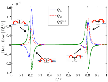
The behavior of the heat flux at the two reservoirs, along with within a period, is shown in Fig. 2 for reservoirs at finite temperature and a small applied bias voltage .
Figure 2: Heat fluxes at the left (solid lines) and right (dashed lines) reservoirs as well as the flux (circles) for a driven level connected to reservoirs at finite temperature and with a small applied bias . The energy of the level evolves in time as with . Parameters: , , and the hybridization are and . Energies are expressed in units of .
Sketches illustrating the physical processes as function of time are also provided. In each case, the horizontal central line indicates the position of the level at a given time referred to the position of the chemical potentials of the reservoirs, while the red arrows indicate the direction of the heat flux associated to the reservoirs.
For the energy of the level is above the highest chemical potential . As evolves, the energy of level approaches from above and when a heat flux leaves the left reservoir, traveling through the central level towards the right reservoir. When the energy of the level becomes approximately aligned with the mean chemical potential of the reservoirs, the heat flow
goes from the central piece into the two reservoirs. Later, the level lies well below the lowest chemical potential and the heat flux becomes vanishingly small. When the level oscillation completes half a period (), the motion reverses and approaches from below. For , a heat flux is established from the reservoirs to the central piece until the level aligns with the mean chemical potential. Then, the heat flows from the central system into the reservoirs.
It is interesting to analyze the total entropy production of the above processes as a function of time. Let us start by
noticing that and . Then, from Eqs. (56) and (C) for the dissipated power in the adiabatic regime, it follows that and therefore
(73)
As discussed in Sec. IV.4, the instantaneous rate of entropy production contains terms associated to the heat production in the reservoirs as well as terms
associated to the heat production at the central piece, as explicitly defined in Eq. (48).
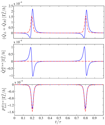
While in Fig. 2 each of these contributions is separately analyzed, in Fig. 3 we show the combined effect.
Figure 3: The different components of the total heat production as a function of time for a single level coupled to two reservoirs within the adiabatic regime. Dashed lines corresponds to reservoirs at , while solid lines are for . Other parameters are the same as in Fig. 2. Energies are expressed in units of . The upper panel shows that the heat flux at the reservoirs is positive and equal to at and may attain negative values at finite temperature. The dissipative heat flux at the driven dot , in the second panel, vanishes when . The bottom panel shows the total dissipative power .
Interestingly, for , which can be exactly verified by noticing that the coefficients entering (VI.2) contain integrands with
at . The physical explanation to this property is the fact that for all the dissipation takes
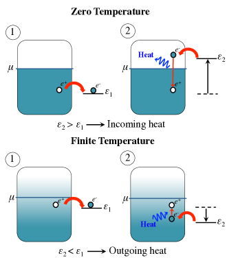
place at the reservoirs. In fact, for reservoirs at zero temperature, heat can only be injected from the central system into the reservoirs, which means that
. However, at finite temperature, the reservoirs can be temporarily cooled down as shown in Fig. 4 and we could have
. In that case, the only possibility to have is to have a positive non-vanishing
. This is illustrated in Fig. 3, where the behavior of the total dissipated power is also shown.
Figure 4: Sketches illustrating the heat exchange between the reservoirs and the central piece. The upper panel corresponds to , in which case the heat generated by the driving can only be injected into the reservoir. The lower panel corresponds to finite temperature and indicates that depending on the position of the level relative to the chemical potential of the reservoir, heat flow can be inwards or outwards.
VI.3 Instantaneous Joule law in the adiabatic regime
In Ref. us we showed that the heat production by a single driven dot connected to a single reservoir at obeys an instantaneous Joule Law in the adiabatic regime.
The corresponding resistance is universal and equal to the charge relaxation resistance introduced in Ref. Buttiker:1993bw, and observed in Ref. Gabelli:2006eg, .
We are interested now in analyzing a possible relation in the case of a dot connected to two reservoirs that may have a finite temperature and a bias voltage. We rely again on linear response.
The term describes the heat dissipated due to the variation in time of the ac potential, and captures the effect of the applied static bias .
The first term, which is proportional to , can be expressed in a different way by evaluating the charge current entering the system up to first order in the velocity as
(74)
For this, we used the relation given by Eq. (22) and the expression for the currents entering the reservoirs, Eq. (65), and follow the steps presented in Appendix B for the slow driving case. Now, combining Eq. (74) with the first term of Eq. (56) we get
(75)
where we have defined the resistance
(76)
which is a manifestly positive quantity at all times.
Therefore, we find that the heat dissipated due to pumping is given by a Joule law with an instantaneous resistance .
This quantity becomes nonuniversal at finite temperatures, which agrees with the finite-temperature result of Ref. Buttiker:1993bw .
If the temperatures of the reservoirs are small compared to their Fermi energy, it is possible to apply the Sommerfeld expansion up to order . Accordingly, we investigate the behavior of at finite temperature
(77)
Remarkably, the resistance becomes universal at , recovering the quantum of charge relaxation resistance . For low but finite
temperatures, the resistance increases as shown in Eq. (77) and becomes . This is illustrated in Fig. 5. The departures from the ideal quantum limit of the resistance are
and are sizable for those times when the energy of the level differs from the mean chemical potential of the reservoirs in an amount .
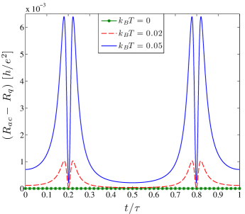
Figure 5: Difference between the ac resistance and the relaxation resistance quantum as a function of time within the adiabatic regime, and for different temperatures . Other parameters are the same as in Fig. 2. Our results show that the instantaneous ac resistance becomes universal only at , attaining the value . For finite temperatures, we have , hence the difference between the two is always a positive quantity.
On the other hand, for the quadratic term in the bias drop of Eq. (56), we also have an instantaneous Joule law of the form
(78)
with an electrical conductance .
VII Conclusions
We have analyzed the dynamics of the energy transport and entropy production in an electron system coupled to multiple reservoirs and slightly driven out of equilibrium by means of ac local and dc bias voltages.
We have formulated an exact quantum dynamical approach, which allows to identify time-resolved quantities, such as the total heat dissipated by the system, the work done on a system, and the entropy production, in a way which is fully consistent with the first and the second laws of thermodynamics.
In addition, we identified conservative and dissipative contributions to the total heat flux and the corresponding contributions to the entropy production.
The time-resolved heat fluxes flowing through the different pieces of the device were investigated in detail.
We have shown that the definition of the time-resolved heat current flowing into the reservoirs recently introduced in Ref. us for a single-terminal system is also suitable for multiterminal devices.
This definition takes into account the energy temporarily stored in the contact region connecting the driven central system and the reservoirs.
Using this definition, we showed that in the limit of a slow driving the first and the second laws of thermodynamics can be formulated consistently at each instant of time.
We illustrated our approach by considering a simple example—a slowly driven resonant level coupled to two electron reservoirs at a finite temperature and with an applied bias voltage.
We showed that at finite temperatures, when one of the reservoirs can be temporarily cooled, the total heat production at each time is positive, hence the entropy production is positive, only if the energy stored in the contact and central regions are taken into account. Since all the equations of Sec. III, IV and V have been derived under very general assumptions regarding the nature of the specific model, we
expect that the qualitative features in the behavior of the entropy production and instantaneous heat flow presented in Sec. VI will remain valid even for different types of periodic driving and also
the case of a quantum dot with many-body interactions.
The latter type of interactions may, however, affect other more quantitative features such as the behavior of the instantaneous Joule law analyzed in Section VI.C, since an electron-electron interaction is shown to affect the charge relaxation resistance at finite temperatures Nigg:2006kl , for large cavities Mora:2010hw and at finite magnetic fields Filippone:2011fy .
Our results thus represent a significant advance toward a full understanding of dissipation and dynamics in quantum electron systems and might have important implications for nanoelectronics and quantum thermodynamics.
VIII Acknowledgements
This work was supported by MINECO under Grant No. FIS2014-52564, UBACyT, CONICET and MINCyT, Argentina.
Here, the term in Eq. (A) which is accompanied by does not contribute due to the difference between the Fermi functions.
Then, after some algebra and by comparing with Eq. (VI.1) we find
(83)
where is given in Eq. (42) and includes in the definition the contributions due to the contacts.
Appendix B Slow driving and small bias voltage
To calculate up to and the currents (65), (VI.1), and the power (VI.1), we need to perform an expansion of the Fermi function entering the integrands as
(84)
and
(85)
where is the Fermi-Dirac distribution if we take the chemical potential and the base temperature as a reference.
In the slow driving regime, for which the typical frequency of the ac potential , it is possible to do an exact analysis by expanding the Green function
(86)
or equivalently the scattering matrix, in powers of us ; mb ; florlili .
By keeping terms up to first order in we get
(87)
In the case of the driven single level, the above expression reduces to
(88)
where is the frozen Green function.
Equation (88) is in fact quite general if the driving does not break the symmetry of scattering with respect to a spatial direction reversal mbook .
Appendix C Coefficients of the adiabatic expansion
By using the low frequency expansion detailed in Appendix B in the expressions of the charge current and the power developed by the ac forces we can calculate
(90)
where , since we take the left reservoir as a reference. We have used the notation
and , as well as the property with . The local frozen density of states can be expressed as
(91)
with being the frozen Green function describing the regime in which the electrons instantaneously adjust its potential to the ac field, and is the total hybridization with the reservoirs.
Following a similar procedure in Eq. (VI.1), we can compute up to second order in . The result is collected in the coefficients , which can be expressed as
(92)
for the first order, and
(93)
for the second order.
Similarly, the coefficients entering the expansion of read
(94)
References
(1)J-P Brantut, C. Grenier, J. Meineke, D. Stadler, S. Krinner, C. Kollath, T. Esslinger, and A. Georges, Science 342, 713 (2013)
(2)G.A. Steele, A.K. Hüttel, B. Witkamp, M. Poot, H.B. Meerwaldt, L.P. Kouwenhoven, and H.S.J. van der Zant, Science 325, 1103 (2009).
(3) C. Lotze, M. Corso, K. J. Franke, F. von Oppen, J. I. Pascual, Science 338, 779 (2012)
(4)
F. Michelini, K. Beltako, A. Crépieux, SPIE Newsroom (2016), \doi10.1117/2.1201601.006320.
(5)D. Segal and A. Nitzan, Phys. Rev. E 73, 026109 (2006).
(6)L. Arrachea, M. Moskalets, and L. Martin-Moreno, Phys. Rev. B 75, 245420 (2007).
(7)
L.-A. Wu and D. Segal, J. Phys. A: Math. Theor. 42, 025302 (2009).
(8) R. Bustos-Marun, G. Refael and F. von Oppen, Phys. Rev. Lett. 111 060802 (2013)
(9)R. Biele, R. D’Agosta and A. Rubio, Phys. Rev. Lett. 115, 056801 (2015)
(10)
M. Carrega, P. Solinas, A. Braggio, M. Sassetti, and U. Weiss, New Journal of Physics 17, 045030 (2015).
(11)
J. Chen, M. ShangGuan, and J. Wang, New Journal of Physics 17, 053034 (2015).
(12)
M. Campisi, J. Pekola, and R. Fazio, New Journal of Physics 17, 035012 (2015).
(13) M.F. Ludovico, F. Battista, F. von Oppen and L. Arrachea, Phys Rev B 93, 075136 (2016).
(14)
K. Proesmans, B. Cleuren, and C. Van den Broeck, J. Stat. Mech. 2016, 023202 (2016).
(15)
A. M. Daré and P. Lombardo, Phys. Rev. B 93, 035303 (2016).
(16)
A. Bruch, M. Thomas, S. Viola Kusminskiy, F. von Oppen, and A. Nitzan,
Phys. Rev. B 93, 115318 (2016).
(17) C. Jarzynski, Phys. Rev. Lett.
78, 2690 (1997).
(18)G. E. Crooks, Phys. Rev. E
60, 2721 (1999).
(19) J. Kurchan, J. Stat. Mech. P07005 (2007).
(20)K. Saito and A. Dhar, Phys. Rev. Lett. 99, 180601 (2007).
(21)
K. Saito and Y. Utsumi, Phys. Rev. B 78, 115429 (2008).
(22)
H. Förster and M. Büttiker, Phys. Rev. Lett. 101, 136805 (2008).
(23)
D. Sánchez, Phys. Rev. B 79, 045305 (2009).
(24)M. Esposito, U. Harbola, and S. Mukamel, Rev. Mod. Phys.
81, 1665 (2009).
(25)M. Esposito, R. Kawai, K. Lindenberg and C. Van den Broeck, Phys. Rev. Lett. 105, 150603 (2010).
(26)
S. Nakamura, Y. Yamauchi, M. Hashisaka, K. Chida, K. Kobayashi, T. Ono, R. Leturcq, K. Ensslin, K. Saito, Y. Utsumi, and A. C. Gossard, Phys. Rev. Lett. 104, 080602 (2010).
(27)M. Campisi, P. Hänggi, and P. Talkner, Rev. Mod. Phys.
83, 771 (2011).
(28)
R. López, J. S. Lim, and D. Sánchez,
Phys. Rev. Lett. 108, 246603 (2012).
(29)
C. Wang and D. E. Feldman,
Phys. Rev. Lett. 110, 030602 (2013)
(30)
Y. Utsumi, O. Entin-Wohlman, A. Aharony, T. Kubo, and Y. Tokura,
Phys. Rev. B 89, 205314 (2014).
(31)R. Uzdin, A. Levy, and R. Kosloff, Phys. Rev. X
5, 031044 (2015).
(32)K. Brandner and U. Seifert, ArXiv:1604.03411 (2016).
(33) U. Seifert, Phys. Rev. Lett. 116, 020601 (2016).
(34)D. Segal, Phys. Rev E 90, 012148 (2014).
(35)M. Carrega, P. Solinas, M. Sassetti, and U. Weiss, Phys. Rev. Lett. 116, 240403 (2016).
(36)R. Schmidt, M. F. Carusela, J. P. Pekola, S. Suomela, and
J. Ankerhold, Phys. Rev. B
91, 224303 (2015).
(37)L. Arrachea, E. R. Mucciolo, C. Chamon, and R. B. Capaz, Phys. Rev. B
86, 125424 (2012).
(38)R. Tuovinen, N. Säkkinen, D. Karlsson, G. Stefanucci and R. van Leeuwen, Phys. Rev. B 93, 214301 (2016).
(39)N. Beraha, A. Soba and M. F. Carusela, arXiv:1604.07714 (2016).
(40) M. F. Ludovico, J. S. Lim, M. Moskalets, L. Arrachea, and D. Sánchez,
Phys. Rev. B 89, 161306(R) (2014).
(41)
R. Balian, From Microphysics to Macrophysics (Springer-Verlag, Berlin, 1982), vol. I, ch. 5.
(42)J. Rammer, Quantum Field Theory of Non-equilibrium States
(Cambridge University Press, New York, 2007).
(43)
G. D. Mahan, Many-Particle Physics (Kluwer/Plenum, New York, 2000), ch. 3.
(44)
J. Ankerhold and J. P. Pekola, Phys. Rev. B 90, 075421 (2014).
(45)
M. Esposito, M. A. Ochoa, and M. Galperin, Phys. Rev. Lett. 114, 080602 (2015).
(46)
G. Rosselló, R. López, and J. S. Lim,
Phys. Rev. B 92, 115402 (2015).
(47) L. Arrachea, Phys. Rev. B 72, 125349 (2005)
(48) L. Arrachea,
Phys. Rev. B, vol. 75, 035319 (2007)
(49) L. Arrachea and M. Moskalets, Phys. Rev. B 74, 245322 (2006).
(50)
M. Büttiker, H. Thomas, A. Prêtre, Mesoscopic capacitors, Phys. Lett. A 180, 364–369 (1993).
(51)
J. Gabelli, G. Fève, J.-M. Berroir, B. Plaçais, A. Cavanna, E. al, Y. Jin, and D. C. Glattli, Science 313, 499–502 (2006).
(52)
S. E. Nigg, R. López, and M. Büttiker, Phys. Rev. Lett. 97, 206804 (2006).
(53)
C. Mora and K. Le Hur, Nature Phys. 6, 697 (2010).
(54)
M. Filippone, K. Le Hur, and C. Mora, Phys. Rev. Lett. 107, 176601 (2011).
(55)
M. Büttiker, Phys. Rev. B 46, 12485 (1992).
(56) M. Moskalets, Scattering matrix Approach to Non-Stationary Quantum Transport, World Scientific, London, 2012.
(57)
F. Battista, M. Moskalets, M. Albert, and P. Samuelsson, Phys. Rev. Lett. 110, 126602 (2013).
(58)
J. S. Lim, R. López, and D. Sánchez, Phys. Rev. B 88, 201304 (2013).
(59)
F. Battista, F. Haupt, and J. Splettstoesser, Phys. Rev. B 90, 085418 (2014).
(60) D.S. Fisher and P.A. Lee, Phys. Rev. B 23, 6851 (1981).
(61) M. Moskalets and M. Büttiker, Phys. Rev. B
69, 205316 (2004).
(62)M. F. Ludovico and L. Arrachea, Phys. Rev. B 87, 115408
(2013).