Kernel-based Sensor Fusion with Application to Audio-Visual Voice Activity Detection

Abstract

In this paper, we address the problem of multiple view data fusion in the presence of noise and interferences. Recent studies have approached this problem using kernel methods, by relying particularly on a product of kernels constructed separately for each view. From a graph theory point of view, we analyze this fusion approach in a discrete setting. More specifically, based on a statistical model for the connectivity between data points, we propose an algorithm for the selection of the kernel bandwidth, a parameter, which, as we show, has important implications on the robustness of this fusion approach to interferences. Then, we consider the fusion of audio-visual speech signals measured by a single microphone and by a video camera pointed to the face of the speaker. Specifically, we address the task of voice activity detection, i.e., the detection of speech and non-speech segments, in the presence of structured interferences such as keyboard taps and office noise. We propose an algorithm for voice activity detection based on the audio-visual signal. Simulation results show that the proposed algorithm outperforms competing fusion and voice activity detection approaches. In addition, we demonstrate that a proper selection of the kernel bandwidth indeed leads to improved performance.

I Introduction

Multiple view data fusion is the process of obtaining a unified representation of data captured in multiple measurement systems of different types. Data fusion has recently attracted a growing interest in the signal processing and data analysis communities due to an extensive use of multiple sensors in everyday devices such as computers and smartphones. Often, data measured in multiple views is contaminated with noises and interferences which are view specific, and fusing the views may allow for obtaining representations of the data, which are robust to the interferences. A challenging example which we consider in the current work is the fusion of audio and visual recordings of a speaker. While each view (audio or video) possibly consists of view-specific interferences (e.g., acoustic noises or face movements), their fusion may give rise to a robust representation of the speech.

In this paper, we use a kernel based geometric approach to address the problem of multiple view data fusion. Classical methods, e.g., those presented in [1, 2, 3, 4, 5], represent a class of non-linear dimensionality reduction methods designed for data measured in a single view. By learning geometric structures of high dimensional data, these methods provide low dimensional representations of the data via eigenvalue decomposition of an affinity kernel. The low dimensional representations preserve the geometry of the data, i.e., local affinities between data points, and they are successfully used in a wide range of applications such as anomaly and target detection and speech enhancement [6, 7, 8, 9]. However, when the data is corrupted by structured interferences, the kernel methods learn the structure of the interferences along with the structure of the data. Therefore, the obtained low dimensional representation retains the relations between the data and the interferences, and, as a result, the kernel methods have a limited robustness to the interferences.

The potential of improving the robustness of the obtained representations to interferences by fusing data captured in multiple views, has recently motivated researchers extending kernel-based geometric methods to the multiple views case [10, 11, 12, 13, 14, 15, 16, 17, 18, 19, 20, 21]. Among these studies, we mention the studies presented in [12, 16, 20, 21] sharing similar ideas of constructing separate affinity kernels for each view, and fusing the data by the product between the affinity kernels. A method of particular interest in this work was presented in [21], where special emphasis is given to the robustness of the fusion process to interferences. The authors presented a data fusion method termed alternating diffusion maps, which is based on fusing the views by multiplying between affinity kernels interpreted as employing separate diffusion processes on each view in an alternating manner. By analyzing the method in the continuous setting, it is shown that the interruptions of a certain view are attenuated by the diffusion steps of the other views.

The ability of kernel methods to properly learn the geometric structure of the data is highly dependent on the selection of the kernel bandwidth, which also has important implications on the robustness of the methods to interferences. The kernel bandwidth, also called the scale parameter, defines a local neighborhood such that all data points within the neighborhood are considered similar, i.e., close to each other. It has an intuitive interpretation by viewing the kernel methods from the graph theory point of view, which we adopt throughout this paper. The affinity kernel defines a graph whose nodes are the data points and the edges are given by the affinities between the data points. Accordingly, all data points located within a local neighborhood defined by the kernel bandwidth are considered connected on the graph. In the single view case, the kernel bandwidth is chosen according to a trade-off. On the one hand, it has to be large enough keeping the graph connected, which is a necessary condition for learning the geometry of the data [22, 5, 23, 24]. On the other hand, the kernel bandwidth has to be as small as possible so that data and interferences will not share the same local neighborhoods [25]. In the multiple view case, the selection of the kernel bandwidth is not addressed in the literature, and the kernel bandwidths are naively chosen in previous studies as if the data is measured in a single view.

In this study, we address the fusion problem of data obtained in multiple views. We revisit the alternating diffusion maps method and analyze it from a different point of view than in [21] using a discrete setting. By adopting ideas from [12, 26], we study how connected data points on graphs of each view affect the connectivity of the graph obtained by fusing the views via the product of the affinity kernels. By assuming a statistical model on the connectivity between data points in each view, we use a simple argument to show that the kernel bandwidth of each view may be chosen such that the graph defined on each single view is not connected. This allows us to use significantly smaller kernel bandwidths improving the robustness of the fusion process to interferences. Based on the introduced statistical model, we propose an algorithm for the selection of the kernel bandwidth. We note that throughout this paper we consider the selection of the kernel bandwidth for the alternating diffusion maps method presented in [21]. However, the provided analysis and the proposed algorithm may be extended with mild modifications to the methods presented in [12, 16, 20], which are also based on the product between the affinity kernels of the views.

Using the alternating diffusion mas with the new algorithm for determining the kernel bandwidth, we address the problem of audio-visual voice activity detection, where the goal is to detect segments of the measured signal containing active speech. We consider a challenging setup in which a speech signal is measured by a single microphone and a video camera in the presence of high levels of acoustic noises and transients, which are short term interruptions, e.g., keyboard taps and office noise [27, 28]. In the video signal, there exist natural mouth movements during non-speech periods which wrongly appear similar to speech. The alternating diffusion maps method is particularly suitable for the fusion of the audio-visual data in this setup since it integrates out the interferences, which are view specific, i.e., transients measured in the microphone and non-speech mouth movements measured by the camera. Based on the alternating diffusion maps method, we propose a data-driven algorithm for voice activity detection. The algorithm comprises a simple preprocessing stage of feature extraction and does not require post-processing, and, in contrast to the method we presented in [29], it requires no training data. Our simulation results demonstrate improved performance of the proposed algorithm compared both to a similar algorithm based on a traditional selection of the kernel bandwidth and compared to competing fusion schemes.

The remainder of the paper is organized as follows. In Section II, we briefly review the alternating diffusion maps method. In Section III, we analyze the method in a discrete setting using tools from graph theory, and propose an algorithm for kernel bandwidth selection. In section IV we address the problem of audio-visual voice activity detection and propose an algorithm based on the alternating diffusion maps method. The improved performance of the proposed algorithm is demonstrated in Section V.

II Review of The Alternating Diffusion Maps Method

Consider a dataset of $N$ samples captured in two different views given by:

$$\left(\mathbf{v}_{1},\mathbf{w}_{1}\right),\left(\mathbf{v}_{2},\mathbf{w}_{2}\right),...,\left(\mathbf{v}_{N},\mathbf{w}_{N}\right),$$ (1)

where $\mathbf{v}_{n}\in\mathbb{R}^{L_{v}}$ and $\mathbf{w}_{n}\in\mathbb{R}^{L_{w}}$ are the $n$th data points of the first and the second views, respectively. An example we will address under this setup is an audio-visual recording of a speaker, where $\mathbf{v}_{n}$ is the $n$th time frame of the signal captured in a microphone and $\mathbf{w}_{n}$ is the corresponding video frame of the mouth region of the speaker. The alternating diffusion maps method presented in [21] is a kernel based geometric method for data fusion. It is designed to reveal the geometric structure of the data, which is mutual to the two views ignoring the interferences, which are captured only in one of the views. In the following, we shortly describe the construction of alternating diffusion maps. Let $\mathbf{K}_{v}\in\mathbb{R}^{N\times N}$ be an affinity kernel representing affinities between data points in the first view, such that the $\left(n,m\right)$th entry of the matrix, denoted by $K_{v}(n,m)$ is given by:

$$K_{v}(n,m)=\exp\left(-\frac{||\mathbf{v}_{n}-\mathbf{v}_{m}||^{2}}{\epsilon_{v}}\right),$$ (2)

where $\epsilon_{v}$ is the kernel bandwidth whose selection is discussed in details in Section III. The affinity kernel $\mathbf{K}_{v}$ in (2) defines a graph on the dataset in the first view such that each data point is a vertex and $K_{v}(n,m)$ is the weight of the edge between vertex $n$ and vertex $m$. Let $\mathbf{M}_{v}\in\mathbb{R}^{N\times N}$ be a row stochastic Markov matrix given by normalizing the rows of $\mathbf{K}_{v}$:

$$\mathbf{M}_{v}=\mathbf{D}_{v}^{-1}\mathbf{K}_{v},$$ (3)

where $\mathbf{D}_{v}\in\mathbb{R}^{N\times N}$ is a diagonal matrix, whose $m$th element on the diagonal is denoted by $D_{v}(m,m)$ and is given by $D_{v}(m,m)={\displaystyle\sum_{n=1}^{N}K_{v}(n,m)}$. In this study, we use a row normalization rather than a column normalization used in [21] allowing us to facilitate the discussion and results in Section III, and our experimental results showed a negligible effect on the type of the normalization. The matrix $\mathbf{M}_{v}$ defines a Markov chain on the graph such that $\mathbf{M}_{v}(n,m)$ is the probability of moving from data point $n$ to data point $m$ in a single step. Similarly to $\mathbf{K}_{v}$, let $\mathbf{K}_{w}\in\mathbb{R}^{N\times N}$ be a matrix representing affinities between data points in the second view, and let $\mathbf{M}_{w}\in\mathbb{R}^{N\times N}$ be the corresponding row stochastic matrix. The views are fused by constructing a unified matrix, which is denoted by $\mathbf{M}$ and is given by the product of the row stochastic matrices [21]:

$$\mathbf{M}=\mathbf{M}_{v}\cdot\mathbf{M}_{w}.$$ (4)

The matrix $\mathbf{M}$ is also row stochastic and it integrates the relations between the data points over the two views; therefore, we term it the multiple view Markov matrix. The continuous counterparts of the matrices $\mathbf{M}_{v}$ and $\mathbf{M}_{w}$ in (4) are typically considered in the literature as diffusion operators [5]. Likewise, the authors in [21] considered $\mathbf{M}$ as an alternating diffusion operator consisting of two diffusion steps on the two views, and showed that this alternating diffusion attenuates the view-specific interferences. In Section IV, we describe the construction of a unified low dimensional representation of the data through the eigenvalue decomposition of the matrix $\mathbf{M}$ similarly to obtaining a low dimensional representation of the data in a single view using principal component analysis.

III Graph Theory Interpretation For Kernel Bandwidth Selection

Recall that the affinity kernel $\mathbf{K}_{v}$ in (2) defines a graph on $\left\{\mathbf{v}_{n}\right\}_{n=1}^{N}$ such that each data point $\mathbf{v}_{n}$ is a vertex and $K_{v}(m,n)=\exp\left(-\frac{||\mathbf{v}_{n}-\mathbf{v}_{m}||^{2}}{\epsilon_{v}}\right)$ is the weight of the edge between vertex $n$ and vertex $m$. The kernel bandwidth $\epsilon_{v}$ controls the connectivity of the graph. When $||\mathbf{v}_{n}-\mathbf{v}_{m}||^{2}<\epsilon_{v}$, high similarities are obtained between data points $n$ and $m$, and they are considered connected; when $||\mathbf{v}_{n}-\mathbf{v}_{m}||^{2}\gg\epsilon_{v}$ the similarity between the points is negligible and we assume no edge between the points. In order to capture the geometric structure of the data, common practice is to set the kernel bandwidth such that each data point is connected to at least one other point, i.e.:

$$\epsilon_{v}>\max_{m}\left[\min_{n}\left(||\mathbf{v}_{n}-\mathbf{v}_{m}||^{2}\right)\right].$$ (5)

This choice is a necessary condition for the graph defined on the dataset to be connected such that there exists a path between every pair of points. In turn, a connected graph is a necessary condition for the eigenvectors of the affinity kernel to form a discrete orthogonal basis. This property is typically used for the construction of low dimensional representations [5, 24]. Yet, the kernel bandwidth should be sufficiently small to prevent the association of data points with different content. In [25], the authors proposed choosing the value of the kernel bandwidth by:

$$\epsilon_{v}=C\cdot\max_{m}\left[\min_{n}\left(||\mathbf{v}_{n}-\mathbf{v}_{m}||^{2}\right)\right],$$ (6)

where $C$ is a parameter which is set in the range of $2\div 3$ to guarantee that the graph is connected in the single view case such that typically each point is connected to several other points. In this study, we focus on the selection of the kernel bandwidth according to (6), yet other existing methods for the kernel bandwidth selection, e.g., those presented in [22, 24, 30], also rely on similar graph connectivity.

In the multiple view case, the kernel bandwidth in each view is typically set in the literature as if the data is captured only in a single view and also require graph connectivity for each view, e.g, in [12, 16, 20, 21]. In contrast, we show that when the data is measured in multiple views, the graph of each single view does not necessarily have to be connected.

To demonstrate this idea, we consider a multiple view graph, which is defined by the Markov matrix $\mathbf{M}$ in (4). The vertices of the graph are pairs of data points $\left\{\left(\mathbf{v}_{n},\mathbf{w}_{n}\right)\right\}_{n=1}^{N}$, and the matrix $\mathbf{M}$ defines a Markov chain on this graph such that the $(n,m)$th entry of $\mathbf{M}$ is the probability of a transition from vertex $n$ to vertex $m$. For simplicity, we relate to (say) vertex $n$ as to point $n$ even though it is related to the pair of points $\left(\mathbf{v}_{n},\mathbf{w}_{n}\right)$. The matrix $\mathbf{M}$ aggregates the relations between the data points based on the two views; there exists an edge between point $n$ and point $m$ in the multiple view graph if the transition probability between them, given by $\mathbf{M}(n,m)$, is non-zero. To capture the geometric structure of the data, the necessary condition that each point is connected to at least one other point applies to the multiple view graph and not to the graphs of the single views. Namely, the single view graphs can be disconnected while each point in the multiple view graph is connected as demonstrated by Proposition 1.

Proposition 1.

$\forall n,\,\exists m\neq n$ such that $M(n,m)\neq 0$ iff $\forall n,\,\exists m\neq n$ such that $M_{v}(n,m)\neq 0$ or $M_{w}(n,m)\neq 0$.

Proposition 1 implies that each point in the multiple view graph is connected if it is connected at least in one of the views.

Proof:

If point $n$ is disconnected in the first view, the $n$th row of the affinity kernel of the first view $\mathbf{K}_{v}$ is given by:

$$\begin{array}[]{c}\left(K_{v}(n,1),K_{v}(n,2),...,K_{v}(n,n),...,K_{v}(n,N)\right)=\\ \,\,\,\,\,\,\,\,\,\,\,\,\,\,\,\,\,\,\,\,\,\,\,\,\,\,\,\,\,\,\,\,\,\,\,\,\,\,\,\,\,\,\,\,\,\,\,\,\,\,\,\,\,\,\,\,\,\,\,\,\,\,\,\,\,\,\,\,\,\,\,\,\,\,\,\,\,\,\,\,\,\,\,\,\,\,\,\,\,\,\,\,\,\left(0,0,...,1,...0\right).\end{array}$$

Consequently, the $n$th row of the corresponding row stochastic Markov matrix $\mathbf{M}_{v}$ is given by:

$$\begin{array}[]{c}\left(M_{v}(n,1),M_{v}(n,2),...,M_{v}(n,n),...,M_{v}(n,N)\right)=\\ \,\,\,\,\,\,\,\,\,\,\,\,\,\,\,\,\,\,\,\,\,\,\,\,\,\,\,\,\,\,\,\,\,\,\,\,\,\,\,\,\,\,\,\,\,\,\,\,\,\,\,\,\,\,\,\,\,\,\,\,\,\,\,\,\,\,\,\,\,\,\,\,\,\,\,\,\,\,\,\,\,\,\,\,\,\,\,\,\,\,\,\,\,\left(0,0,...,1,...0\right).\end{array}$$

According to (4) and by the rule of matrix product, the $n$th row of $\mathbf{M}$ is given by:

$$\begin{array}[]{c}\left(0,0,...,1,...0\right)\cdot\mathbf{M}_{w}=\\ \left(M_{w}(n,1),M_{w}(n,2),...,M_{w}(n,n),...,M_{w}(n,N)\right).\end{array}$$

Therefore, $M(n,m)\neq 0$ iff $M_{w}(n,m)\neq 0$. If point $n$ is connected to (say) point $m$ in the first view, i.e., $M_{v}(n,m)\neq 0$, by the matrix product rule, the $n$th row in $\mathbf{M}$ is given by a linear combination of row $n$ and row $m$ in $\mathbf{M}_{w}$; since $M_{w}(m,m)\neq 0$ (each point is connected to itself), we have that $M(n,m)\neq 0$. ∎

Namely, the necessary condition to learn the geometry of the data from two views is that each point is connected at least in one of the views. Therefore, the kernel bandwidths of each view may be set to small values without satisfying the requirement that the graphs of the single views are connected. We will show in Section V that assigning small values to the kernel bandwidth increases the robustness of the representation obtained using the multiple view affinity kernel to interferences.

The remainder of this section revolves around the selection of the kernel bandwidth. By using a simplifying statistical model for the graph connectivity, we associate the selection of the kernel bandwidth in the single view case with the average number of connections, which we denote by $\delta$. Then we show that in the multiple view case a proper kernel bandwidth is obtained by reducing the number of connections up to a root factor, i.e., $\sqrt{\delta}$. Based on this result, we present an algorithm for the selection of the kernel bandwidths.

Let $\mathds{1}_{v}\left(n,m\right)$ be an indicator which equals one if point $n$ and point $m$ are connected in the first view and zero otherwise. For simplicity, we assume that each pair of data points is connected with probability $p_{v}$ independently from all other data-points in the view. Namely, $\left\{\mathds{1}_{v}\left(n,m\right)\right\}_{n,m}$ are independent and identically distributed (iid) random variables such that:

$$\mathds{1}_{v}\left(n,m\right)=\left\{\begin{array}[]{cc}1,&\text{w.p.}\,p_{v}\\ 0,&\text{otherwise}\end{array}\right\}.$$ (7)

In addition, we assume that the connectivity between data points in a certain view is independent from the connectivity in the other views. We note that these two assumptions do not usually hold in practice. For example, two points being connected to a third point implies that the two points are close to each other, and as a result, they are connected with high probability. In addition, since the data from the different views are measurements of the same phenomenon, high correlation is expected across the views. Yet, we justify these assumptions by considering data contaminated with interferences, and assuming that the interferences reduce these correlations.

Based on this statistical model, the number of connections of a certain point to the other $N-1$ points in the graph of the first view is given by a binomial distribution, denoted by $B_{v}$:

$$B_{v}\left(N-1,p_{v}\right).$$

The parameter $p_{v}$ is directly related to the kernel bandwidth $\sigma_{v}$ in (2); the larger the kernel bandwidth, the higher the probability that two points are connected. We assume that the kernel bandwidth, and therefore $p_{v}$, are chosen such that each point is connected on average to $S_{v}$ points, i.e., $p_{v}\approx\frac{S_{v}}{N-1}$, where $p_{v}\cdot(N-1)$ is the mean value of the binomial distribution. Based on this model, the probability that a certain point is disconnected is denoted by $q_{v}$ and is given by:

$$q_{v}=\left(1-p_{v}\right)^{N-1}.$$

For large values of $N$, we approximate $q_{v}$ by:

$$q_{v}\thickapprox\left(1-\frac{S_{v}}{N-1}\right)^{N-1}\thickapprox e^{-S_{v}}.$$ (8)

We note that we assumed in (8) that the average number of connections $S_{v}$ does not depend on the number of data points $N$. In fact, some studies, e.g., the one presented in [22], suggest setting a constant number of connections to each point regardless to the size of the dataset.

In the single view case, the kernel bandwidth $\epsilon_{v}$ is chosen such that the graph is connected. Under this statistical model, it is equivalent to setting $S_{v}$ such that the probability $q_{v}$ in (8) approaches zero. Namely, setting the kernel bandwidth is equivalent to setting the average number of connections $S_{v}$ to a certain value $\delta$ such that $e^{-\delta}$ approaches zero.

We proceed by considering the multiple view case, in which a similar statistical model is considered for the second view as well. Let $p_{w,}\,S_{w}$ and $q_{w}$ be the equivalents of $p_{v,}\,S_{v}$ and $q_{v}$ in the second view, respectively. We recall that a pair of points, point $n$ and point $m$, is connected in the multiple view graph if the $\left(n,m\right)$th entry of $\mathbf{M}$ in (4) is non-zero. The $(n,m)$th entry is explicitly written as:

$$M\left(n,m\right)={\displaystyle\sum_{l}M_{v}\left(n,l\right)M_{w}\left(l,m\right).}$$

which implies that point $n$ and point $m$ are connected in the multiple view graph if there exists a third point $l$ such that points $n$ and $l$ are connected in the first view and points $l$ and $m$ are connected in the second view. Since the probability that the pair is connected via a third point $l$ is $p_{v}p_{w}$, there will be on average $\left(N-2\right)p_{v}p_{w}$ such points, where for simplicity we assumed that $l\neq n\neq m$. The term $\left(N-2\right)p_{v}p_{w}$ may be rewritten as:

$$\left(N-2\right)p_{v}p_{w}=\left(N-2\right)\frac{S_{v}}{N-1}\frac{S_{W}}{N-1}\approx\frac{S_{v}S_{W}}{N-1},$$

where we neglect the term $\frac{N-2}{N-1}$, which approximately equals one for large values of $N$. Typically, the average number of points connected to a certain point, $S_{v}$ in the first view or $S_{w}$ in the second view, is significantly smaller than $N$. Therefore, we assume that $\frac{S_{v}S_{W}}{N-1}<1$, and we view this term as the probability that point $n$ and point $m$ are connected in the multiple view graph. The number of connections of each point in the multiple view graph is therefore given by the following binomial distribution:

$$B\left(N-1,\frac{S_{v}S_{w}}{N-1}_{v}\right),$$ (9)

and, specifically, each point in the multiple view graph is connected on average to $S_{v}S_{w}$ other points. Based on the binomial distribution and similarly to (8), the probability that a point is disconnected in the multiple view graph, which we denote by $q$, is approximated by:

$$q\thickapprox\left(1-\frac{S_{v}S_{w}}{N-1}\right)^{N-1}\thickapprox e^{-S_{v}S_{W}}.$$

We interpret this result similarly to the result obtained for the single view case; to meet the condition that each point in the graph is connected, the probability $q$ has to approach zero, i.e., $q=e^{-\delta}$ as in the single view case, such that $S_{v}S_{w}=\delta$. Assuming for simplicity that $S_{v}=S_{w}$, the average number of connections in each view should be set to $S_{v}=S_{w}=\sqrt{\delta}$. In summary, in the multiple view case, we may reduce the average number of connections of each point by a root factor, and thus, significantly reduce the size of the kernel bandwidth, while meeting the requirement on the connectivity of the multiple view graph. We will show in Section V that this choice of the kernel bandwidth improves the representation obtained by the multiple view kernel method.

Next, we describe an algorithm for the selection of the kernel bandwidths. For simplicity, we consider the selection of the kernel bandwidth of the first view; the selection of the kernel bandwidth of the second view is equivalent. We start by estimating $\delta$, i.e., the average number of connections, $S_{v}=\left(N-1\right)p_{v}$, when the kernel bandwidth is selected according to (6) as if the data is captured only in a single view. Recalling that $p_{v}$ is the probability that two arbitrary points are connected, we estimate it by:

$$\hat{p}_{v}=\frac{1}{N(N-1)}{\displaystyle\sum_{m}\sum_{n\neq m}K_{v}\left(n,m\right),}$$ (10)

where $\hat{p}_{v}$ is the estimate of $p_{v}$, and $K_{v}(n,m)$ is the $\left(n,m\right)$th entry of the affinity kernel $\mathbf{K}$ in (2). According to (2), $K_{v}\left(n,m\right)$ is in the range of $0\div 1$ and a high value of $K_{v}\left(n,m\right)$ indicates that points $n$ and $m$ are connected. By selecting the kernel bandwidth according to (6) as if the data captured in a single view, the estimate of $\delta$, denoted by $\hat{\delta}$, is given by:

$$\hat{\delta}=\left(N-1\right)\hat{p}_{v}=\frac{1}{N}{\displaystyle\sum_{m}\sum_{n\neq m}K_{v}\left(n,m\right).}$$ (11)

We denote the new bandwidth of the affinity kernel by $\epsilon_{v}^{\text{AD}}$, where AD is alternating diffusion, and we select it such that the estimated average number of connections, which we denote by $\delta^{\text{AD}}$, is reduced to $\sqrt{\hat{\delta}}$. We propose selecting $\epsilon_{v}^{\text{AD}}$ similarly to (6) by:

$$\epsilon_{v}^{\text{AD}}=C^{\text{AD}}\cdot\max_{m}\left[\min_{n}\left(||\mathbf{v}_{n}-\mathbf{v}_{m}||^{2}\right)\right],$$ (12)

where $C^{\text{AD}}$ is a parameter in the range of $0\div C$. The selection of a proper kernel bandwidth is reduced to the selection of the parameter $C^{\text{AD}}$ decreasing the average number of connections by a root factor. We recall that to estimate $\hat{\delta}$ in (11), the parameter $C$ in (6) is chosen in the range of $2\div 3$ (as if the data is captured in a single view), and propose searching the parameter $C^{\text{AD}}$ within a discrete set whose elements lie on a linear grid. Let $\mathcal{C}=\left\{C_{k}\right\}_{k=1}^{\left|\mathcal{C}\right|}$ be a discrete set of size $\left|\mathcal{C}\right|$, where $C_{k},\,k=1,2,...,\left|\mathcal{C}\right|$ are given by $C_{k}=\frac{k}{\left|\mathcal{C}\right|}C$. We propose applying a binary search within the set such that the proposed kernel bandwidth, $C^{\text{AD}}$, is given by the element $C_{k}$ for which the average number of connections $\delta^{\text{AD}}$ is the closest to $\sqrt{\hat{\delta}}$. We summarize the proposed algorithm in Algorithm 1, and note that the kernel bandwidth in the second view is selected similarly.

Algorithm 1 Kernel bandwidth selection

1:Calculate $\epsilon_{v}$ in (6) by setting $C=2\div 3$ as if the data is captured in a single view

2:Calculate $\mathbf{K}_{v}$ in (2)

3:Estimate $\hat{\delta}$ in (11)

4:Define: $\mathcal{C}=\left\{C_{k}\right\}_{k=1}^{\left|\mathcal{C}\right|}$, where $C_{k}=\frac{k}{\left|\mathcal{C}\right|}C$

5:while $|\mathcal{C}|\neq{1}$ do

6:     $C^{\text{AD}}=C_{|\mathcal{C}|/2}$

7:     Estimate $\delta^{\text{AD}}$ similarly to (11) by recalculating $\mathbf{K}_{v}$ with the parameter $C^{\text{AD}}$

8:     if $\delta^{\text{AD}}>\sqrt{\hat{\delta}}$ then

9:         $\mathcal{C}=\left\{C_{k}\right\}_{k=1}^{\left|\mathcal{C}\right|/2}$

10:     else

11:         $\mathcal{C}=\left\{C_{k}\right\}_{k={\left|\mathcal{C}\right|/2+1}}^{\left|\mathcal{C}\right|}$

12:     end if

13:end while

14:Using the obtained $C^{\text{AD}}$, calculate the new kernel bandwidth $\epsilon_{v}^{\text{AD}}$ in (12)

IV Audio Visual Fusion With Application To Voice Activity Detection

We consider speech measured by a single microphone and by a video camera pointed to the face of the speaker. The audio-visual signal is processed in frames, and we consider a sequence of $N$ frames, which are aligned in the two views (audio and video). While speech is measured in the two views, the interruptions are view specific. The audio signal consists of, in addition to speech, background noise and transients, which are short-term interferences, e.g. keyboard taps and office noise; the video signal contains mouth movements during non-speech intervals, which are considered as interferences since they appear similar to speech. Our goal is obtaining a representation of speech, which is robust to noise and interferences. In order to accomplish this goal, we apply alternating diffusion maps, where the kernel bandwidth is determined according to Algorithm 1.

The alternating diffusion maps method is applied in a domain of features, which are designed to reduce the effect of the interferences [29]. The audio signal is regarded as the first view, and it is represented by features based on Mel-Frequency Cepstral Coefficients (MFCC), which are commonly used for speech representation [31]. Specifically, the $n$th data point in the first view, $\mathbf{v}_{n}\in\mathbb{R}^{L_{v}}$ in (1), is the feature vector of the $n$th frame, and is given by the concatenation of the MFCCs of frames $n-1,n,$ and $n+1$. Namely, $L_{v}$ is the total number of the coefficients in three consecutive frames. The use of consecutive frames reduces the effect of transients since speech is assumed more consistent over time compared to transients, which are rapidly varying. The data obtained in the second view, i.e., the video signal, is represented by motion vectors [32] such that the production of speech is assumed associated to high levels of mouth movement. The features representation of the $n$th frame of the video signal, $\mathbf{w}_{n}\in\mathbb{R}^{L_{w}}$, is given by concatenating the absolute values of the motion vectors in frames $n-1,n$ and $n+1$. Similarly to the audio signal, the use of consecutive frames for representation reduces the effect of short-term mouth movements during non-speech intervals. For more details on the construction of the features, we refer the reader to [29].

The representation using the specifically designed features is only partly robust to the interferences. For example, video features of a non-speech frame may be wrongly similar to the features of a speech frame if the former contains large movements of the mouth. To further improve the robustness of the representation to noise, the two views are fused using the alternating diffusion maps method with the improved affinity kernel. Specifically, we construct the affinity kernels of the two views, $\mathbf{M}_{v}$ and $\mathbf{M}_{w}$, according to (2) and (3) using the features $\left\{\mathbf{v}_{n}\right\}_{n=1}^{N}$and $\left\{\mathbf{w}_{n}\right\}_{n=1}^{N}$, respectively, and fuse the views by $\mathbf{M}=\mathbf{M}_{v}\cdot\mathbf{M}_{w}$. Then, we construct an eigenvalue decomposition of $\mathbf{M}$ such that the eigenvectors aggregate the connections between the data points within each view and between the views into a global representation of the data. Since the matrix $\mathbf{M}$ is row stochastic, the eigenvalue with the largest absolute value is $1$ and it corresponds to an all ones eigenvector [5]. This eigenvector is neglected since it does not contain information. We note that the eigenvectors of $\mathbf{M}$ are not guaranteed to be real valued as it is guaranteed for the single view matrices $\mathbf{M}_{v}$ and $\mathbf{M}_{w}$ since the latter are similar to symmetric matrices. Therefore, one solution is constructing an eigenvalue decomposition of the symmetric matrix $\mathbf{M}\mathbf{M}^{T}$. A different approach is obtaining a representation by the singular value decomposition of $\mathbf{M}$ as described in [33]. Yet, our experiments have shown that the eigenvectors corresponding to the several largest eigenvalues of $\mathbf{M}$ are indeed real and that the three approaches perform similarly.

We demonstrate the use of the representation obtained by alternating diffusion maps for the problem of voice activity detection. Let $\mathbb{\mathcal{H}}_{0},\mathbb{\mathcal{H}}_{1}$ be hypotheses of speech absence and speech presence, respectively, and let $\mathds{1}_{n}$ denote a speech indicator at the $n$th frame, given by:

$$\mathds{1}_{n}=\left\{\begin{array}[]{ccc}1&;&\mathcal{H}_{1}\\ 0&;&\mathcal{H}_{0}\end{array}\right\}.$$

Given a sequence of $N$ frames, the goal is to estimate the speech indicator, i.e., to separate the sequence of frames to speech and non-speech clusters. We found in our experiments that the obtained representation of the audio-visual signal, and specifically, its first coordinate, i.e., the leading (non-trivial) eigenvector of the matrix $\mathbf{M}$ in (4), which we denote by $\boldsymbol{\nu}_{1}\in\mathbb{R}^{N}$, successfully separates between speech and non-speech frames. Therefore, we take a similar approach to [34] and estimate the speech indicator by comparing the leading eigenvector to a threshold $\tau$:

$$\hat{\mathds{1}}{}_{n}=\left\{\begin{array}[]{ccc}1&;&\nu_{1}(n)>\tau\\ 0&;&\text{otherwise}\end{array}\right\},$$ (13)

where $\nu_{1}(n)$ in the $n$th entry of the eigenvector $\boldsymbol{\nu}_{1}$, and the threshold may be chosen according to a specific application. We note that the leading eigenvector $\boldsymbol{\nu}_{1}$ is widely used in the literature for clustering and it was shown in [35] that it solves the well-known normalized cut problem. In contrast to previous works, in this study the leading eigenvector is obtained from the multiple view Markov matrix such that it clusters the data according to the two views. Similarly to [34], the leading eigenvector is used as a continuous measure of voice activity rather than for binary clustering. The proposed voice activity detection algorithm is summarized in Algorithm 2. Before proceeding to the experimental results, we note that the proposed representation and hence the speech indicator are obtained in a batch manner assuming that $N$ consecutive frames are available in advance. Yet, as described in [29], a training set may be used to construct the representation, and then it can be extended to new incoming frames, e.g., using the Nyström method, in an online manner [36].

Algorithm 2 Voice activity detection

1:Calculate the features of the audio-visual signal $\left(\mathbf{v}_{1},\mathbf{w}_{1}\right),\left(\mathbf{v}_{2},\mathbf{w}_{2}\right),...,\left(\mathbf{v}_{N},\mathbf{w}_{N}\right)$

2:Calculate $\mathbf{K}_{v}$ and $\mathbf{K}_{w}$ according to (2) and Algorithm 1

3:Calculate $\mathbf{M}_{v}$ and $\mathbf{M}_{w}$ according to (3)

4:Fuse the views by calculating $\mathbf{M}$ in (4)

5:Obtain the leading eigenvector $\boldsymbol{\nu}_{1}$

6:for $n=1:N$ do

7:     if $\nu_{1}(n)>\tau$ then

8:         $\hat{\mathds{1}}{}_{n}=1$

9:     else

10:         $\hat{\mathds{1}}{}_{n}=0$

11:     end if

12:end for

V Simulation Results

We use a dataset that we recently presented in [29]. The signals are recorded using a microphone and a frontal video camera of a smartphone pointed to the face of the speaker. The video signal is processed in $25$ fps and it comprises the region of the mouth of the speaker automatically cropped out from the recorded video as described in [29] and illustrated in Fig. 1. The audio signal is processed in $8$ kHz using time frames of $634$ samples with $50\%$ overlap, such that this setup aligns between the audio and the video signals. The dataset comprises $11$ sequences of different speakers, each of which is $60$ s long containing speech and non-speech intervals.

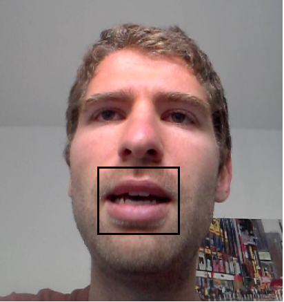
Figure 1: An example of a video frame and the cropped mouth region.

The signals are recorded in a quiet room and we synthetically add different types of background noise and transients to the audio signal. The transients are taken from an online free corpus [37] and they are normalized such that they have the same maximal amplitude as the clean audio signal. Based on the clean audio, we mark the ground truth in each frame, such that frames with energy level higher than $1\%$ of the highest energy level in the sequence are marked as speech frames. This setup of voice detection has a fine resolution of few tens of milliseconds, and it is useful for application such as speech recognition where single phonemes should be isolated [38, 39].

In the first experiment, we evaluate the proposed voice activity detection algorithm, termed “Alternating” in the plots, by comparing it to other versions of the algorithm based only on a single view (audio or video). We term the versions of the algorithm based on the first and the second view “Audio” and “Video”, respectively, and the corresponding speech indicators are estimated by comparing the leading eigenvectors of the matrices $\mathbf{M}_{v}$ in (3) and $\mathbf{M}_{w}$ to a threshold, respectively. In addition, we examine another two approaches for the fusion of the views using the corresponding row stochastic matrices. In the first approach, the fused matrix is given by the Hadamard product between the matrices: $\mathbf{M}_{v}\circ\mathbf{M}_{w}$, where $\circ$ denotes point-wise multiplication, and in the second approach the views are fused by a simple sum: $\mathbf{M}_{v}+\mathbf{M}_{W}$. These approaches are termed in the plots “Hadamard” and “Sum”, respectively. We note that both in the proposed algorithm and in the competing methods, the speech indicator is estimated by the leading eigenvector obtained by the eigenvalue decomposition with an arbitrary sign. To set the sign of the eigenvector, one may for example consider the variability of the video signal over time such that the lack of mouth movement over several consecutive frames indicates absence of speech. In this study, the sign of the eigenvector is assumed to be known for all the methods.

In addition to the different merging schemes, we compare the proposed algorithm to the method presented in [40] termed “Tamura” in the plots. The performances of the algorithms are presented in Fig. 2 for different types of transients in the form of ROC curves, i.e., plots of probability of detection versus probability of false alarms. The larger the Area Under the Curve (AUC) is, the better the performance of the algorithms are, and the AUC of each algorithm is presented in the legend box. It can be seen in the plots that the algorithm based on the video signal provides relatively poor performance compared to the other algorithms. This is mainly since the ground truth is set to a fine resolution, and the video signal is not sensitive enough. For example, video frames of a closed mouth may be measured during both speech and non-speech intervals. We note that in most of the previous studies, the video signal is used for the detection of long speech intervals of several words, and it cannot detect speech in fine resolutions. In addition, we note that we also compared the proposed algorithm to the algorithm we recently presented in [29]. In [29], we proposed a separate representation of each view and estimated voice activity separately based on each representation; then, we fused the views by merging the estimators. However, due to the challenging problem setting considered in this study, for which the speech is detected at a fine resolution, we found that incorporating the visual information as proposed in [29] does not improve the detection scores. Hence the simulation of [29] is not presented in the plots.

The audio signal in Fig. 2 also performs poorly due to the presence of transients, which are not properly separated from speech. The other fusion approaches, “Hadamard” and “Sum” slightly benefit from the fusion of the sensors and provide performances comparable to the performance obtained by audio signal. The proposed fusion of the audio-visual signal provides improved performance and outperforms all the other algorithms.

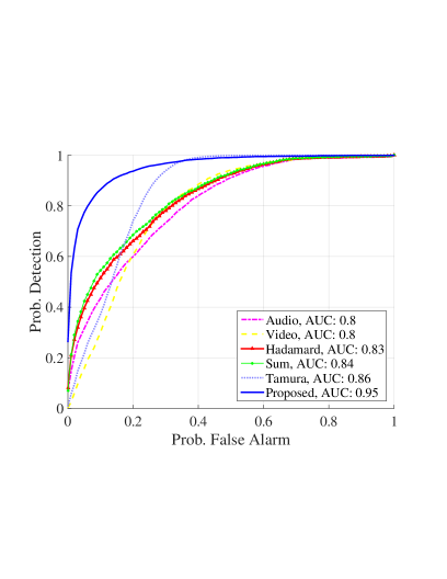
(a)

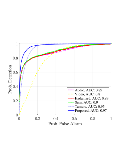
(b)

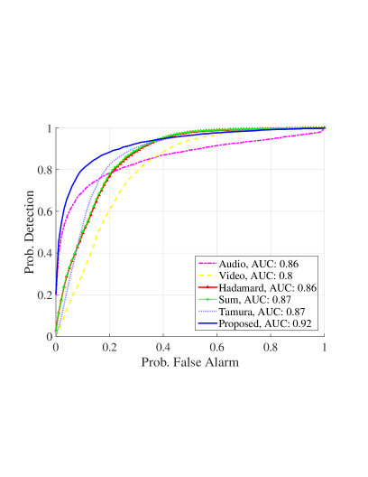
(c)

Figure 2: Probability of the detection vs probability of false alarm. Transient type: (a) hammering, (b) door-knocks, (c) microwave.

To further gain insight on the performance of the proposed algorithm for voice activity detection, we present in Fig. 3 an example of speech detection in a sequence contaminated by hammering. In this experiment, we set the threshold value in (13) to provide $90$ percent correct detection rate and compare the false alarms resulting from the proposed algorithm to the false alarms resulting from the algorithm presented in [40]. As demonstrated in Fig. 3 (top), significantly less false alarms are received by the proposed algorithm compared to the competing detector such that the latter wrongly detects most of the transients as speech.

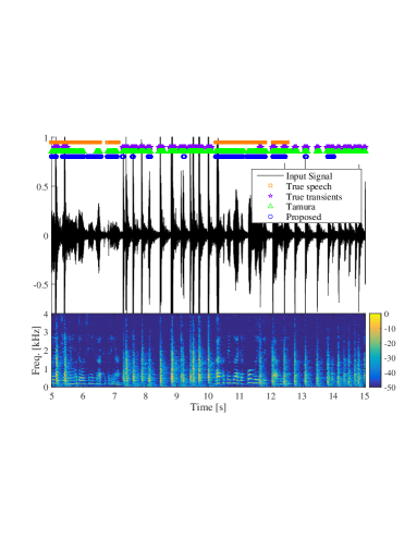
Figure 3: Qualitative assessment of the proposed algorithm for voice activity detection, with a hammering transient. (Top) Time domain, input signal- black solid line, true speech- orange squares, true transients- purple stars, “Tamura” with a threshold set for 90 percents correct detection rate- green triangles, proposed algorithm with a threshold set for 90 percents correct detection rate- blue circles. (Bottom) Spectrogram of the input signal.

In Figs. 2-3, we set $C=2$ in (6) as if the data is obtained in a single view, and we proceed to evaluate the performance of the proposed algorithm for different values of the kernel bandwidth in the next experiment. In Fig. 4 we present plots of the AUC of the proposed voice activity detector versus the parameter $C$ in (6) for different types of noise and interferences. We recall that the parameter $C$ represents the kernel bandwidth such that in the single view case, connected graphs typically correspond to $C$ values in the range $2\div 3$, and disconnected graphs correspond to $C$ values less than $1$. The red solid line in Fig. 4 is obtained by changing only the parameter $C$ related to the audio signal while keeping the parameter related to the video signal fixed (with a constant value $C=2$). The blue dot in the plots is $C^{\text{AD}}$, i.e., the proposed kernel bandwidth obtained by algorithm 1. We empirically found sufficient searching $C^{\text{AD}}$ over a grid with a step of $\frac{C}{\left|\mathcal{C}\right|}=0.05$ such that sweeping the parameter $C^{\text{AD}}$ over values below this scale has negligible effect on the estimated average number of connections in the graph. It can be seen in the plots that by reducing the value of the parameter $C$ the AUC is improved up to a peak obtained when $C\approx 0.5$. The peak value in the plots is the sweet spot in the trade-off in the kernel bandwidth selection. On the one hand, small values of the kernel bandwidth remove wrong connections in the graph between speech and non-speech frames, resulting in a representation in which these frames are better separated. On the other hand, too small kernel bandwidth causes the multiple view graph to be disconnected. Indeed, the significant degradation of the AUC for parameter values below the peak may indicate that the multiple view graph is disconnected such that the obtained audio-visual representation no longer captures the geometric structure of speech. The fact that the peak is obtained for parameter value below $1$ indicates that a better representation of the audio-visual signal is obtained by setting the kernel bandwidth such that the graph of the audio signal is disconnected. These plots demonstrate the idea that the kernel bandwidth should be chosen as the smallest possible keeping the graph of the multiple views connected. In addition, Fig. 4 demonstrate the performance of Algorithm 1 for the selection of the kernel bandwidth. The parameter $C$ obtained by the algorithm, i.e., $C^{\text{AD}}$, successfully provides AUC close to the peak value. The slight deviation of $C^{\text{AD}}$ from the peak may be explained by the assumptions on the statistical model in Section III, which may not hold in practice.

We note that Algorithm 1 is applied to the audio view since we expect to benefit from the algorithm only when there are high levels of noise and interferences. The video signal is considered relatively clean even though there exist some non-speech mouth movements, which may be wrongly detected as speech. In the case of clean signals, audio or video, there are significantly less wrong connections in the graphs of the single views, and hence, reducing the kernel bandwidths does not improve the obtained representation as in the case where the signal is measured in the presence of noises and interferences.

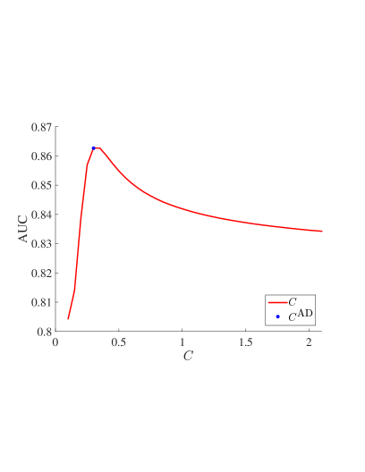
(a)

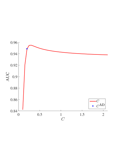
(b)

Figure 4: AUC vs the parameter $C$ of the audio view. (a) background noise: babble noise with $-5$ dB SNR, (b) transient type: keyboard-taps, background noise: colored Gaussian noise with $-5$ dB SNR.

VI Conclusions

We have addressed the problem of multiple view data fusion. We revisited the alternating diffusion maps method and proposed a new interpretation from a graph theory point of view, in which the affinity kernels of the single and multiple views define graphs on the data. By introducing a statistical model of the connectivity between data points on the graphs, we showed that fusing the data by a product of the affinity kernels increases the average number of connections in the multiple view case. Accordingly, the kernel bandwidth, controlling the connectivity between the data points, may be set significantly smaller than in the single view case. Specifically, we showed that the proper kernel bandwidth is the one reducing the average number of connections by a root factor, and presented an algorithm for its selection. Using the alternating diffusion maps method with the improved affinity kernel, we have addressed the problem of audio-visual fusion. In particular, we have considered the task of voice activity detection in the presence of transients; we have shown that the representation obtained by alternating diffusion maps allows for accurate speech detection using the first coordinate, i.e., the leading eigenvector. Our simulation results have demonstrated that the incorporation of visual data significantly improves the detection scores both compared to detecting speech based on only the audio data and compared to alternative merging schemes. In addition, our simulation results have demonstrated that reducing the kernel bandwidth below the values typically used in the single view case improves the robustness of the fusion to transient interferences and consequently the voice activity detection scores. Finally, we have demonstrated that the proposed algorithm for the kernel bandwidth selection allows for selecting near optimal values of the kernel bandwidth.

References

- [1] S. T. Roweis and L. K. Saul, “Nonlinear dimensionality reduction by locally linear embedding,” Science, vol. 290, no. 5500, pp. 2323–2326, 2000.
- [2] M. Balasubramanian, E. L. Schwartz, Tenenbaum J. B., de Silva V., and J. C. Langford, “The isomap algorithm and topological stability,” Science, vol. 295, no. 5552, pp. 7–7, 2002.
- [3] M.l Belkin and P. Niyogi, “Laplacian eigenmaps for dimensionality reduction and data representation,” Neural Computation, vol. 15, no. 6, pp. 1373–1396, 2003.
- [4] D. L. Donoho and C. Grimes, “Hessian eigenmaps: Locally linear embedding techniques for high-dimensional data,” Proc. the National Academy of Sciences, vol. 100, no. 10, pp. 5591–5596, 2003.
- [5] R.R. Coifman and S. Lafon, “Diffusion maps,” Applied and Computational Harmonic Analysis, vol. 21, no. 1, pp. 5–30, 2006.
- [6] G. Mishne and I. Cohen, “Multiscale anomaly detection using diffusion maps,” IEEE Journal of Selected Topics in Signal Processing, vol. 7, no. 1, pp. 111–123, 2013.
- [7] G. Mishne, R. Talmon, and I. Cohen, “Graph-based supervised automatic target detection,” IEEE Transactions on Geoscience and Remote Sensing, vol. 53, no. 5, pp. 2738–2754, 2015.
- [8] R. Talmon, I. Cohen, S. Gannot, and R. R. Coifman, “Supervised graph-based processing for sequential transient interference suppression,” IEEE Transactions on Audio, Speech, and Language Processing, vol. 20, no. 9, pp. 2528–2538, 2012.
- [9] R. Talmon, I. Cohen, and S. Gannot, “Single-channel transient interference suppression with diffusion maps,” IEEE Transactions on Audio, Speech, and Language Processing, vol. 21, no. 1, pp. 132–144, 2013.
- [10] D. Zhou and C. J. C. Burges, “Spectral clustering and transductive learning with multiple views,” in Proceedings of the 24th international conference on Machine learning. ACM, 2007, pp. 1159–1166.
- [11] M. B. Blaschko and C. H. Lampert, “Correlational spectral clustering,” in IEEE Conference on Computer Vision and Pattern Recognition (CVPR), 2008. IEEE, 2008, pp. 1–8.
- [12] V. R. De Sa, P. W. Gallagher, J. M. Lewis, and V. L. Malave, “Multi-view kernel construction,” Machine learning, vol. 79, no. 1-2, pp. 47–71, 2010.
- [13] A. Kumar, P. Rai, and H. Daume, “Co-regularized multi-view spectral clustering,” in Advances in Neural Information Processing Systems, 2011, pp. 1413–1421.
- [14] A. Kumar and H. Daumé, “A co-training approach for multi-view spectral clustering,” in Proceedings of the 28th International Conference on Machine Learning (ICML-11), 2011, pp. 393–400.
- [15] Y. Y. Lin, T. L. Liu, and C. S0 Fuh, “Multiple kernel learning for dimensionality reduction,” IEEE Transactions on Pattern Analysis and Machine Intelligence, vol. 33, no. 6, pp. 1147–1160, 2011.
- [16] B. Wang, J. Jiang, W. Wang, Z. H. Zhou, and Z. Tu, “Unsupervised metric fusion by cross diffusion,” in IEEE Conference on Computer Vision and Pattern Recognition (CVPR), 2012. IEEE, 2012, pp. 2997–3004.
- [17] H. C. Huang, Y. Y. Chuang, and C. S. Chen, “Affinity aggregation for spectral clustering,” in IEEE Conference on Computer Vision and Pattern Recognition (CVPR), 2012. IEEE, 2012, pp. 773–780.
- [18] B. Boots and G. Gordon, “Two-manifold problems with applications to nonlinear system identification,” arXiv preprint arXiv:1206.4648, 2012.
- [19] M. M. Bronstein, K. Glashoff, and T. A. Loring, “Making laplacians commute,” arXiv preprint arXiv:1307.6549, 2013.
- [20] Ofir Lindenbaum, Arie Yeredor, Moshe Salhov, and Amir Averbuch, “Multiview diffusion maps,” arXiv preprint arXiv:1508.05550, 2015.
- [21] R. R. Lederman and R. Talmon, “Learning the geometry of common latent variables using alternating-diffusion,” Applied and Computational Harmonic Analysis, 2015.
- [22] L. Zelnik-Manor and P. Perona, “Self-tuning spectral clustering.,” in NIPS, 2004, vol. 17, p. 16.
- [23] S. Lafon, Y. Keller, and R.R. Coifman, “Data fusion and multicue data matching by diffusion maps,” IEEE Transactions on Pattern Analysis and Machine Intelligence, vol. 28, no. 11, pp. 1784–1797, 2006.
- [24] Ulrike Von Luxburg, “A tutorial on spectral clustering,” Statistics and computing, vol. 17, no. 4, pp. 395–416, 2007.
- [25] Y. Keller, R. R. Coifman, S. Lafon, and S. W. Zucker, “Audio-visual group recognition using diffusion maps,” IEEE Transactions on Signal Processing, vol. 58, no. 1, pp. 403–413, 2010.
- [26] Stefan Steinerberger, “A filtering technique for markov chains with applications to spectral embedding,” arXiv preprint arXiv:1411.1638, 2014.
- [27] A. Hirszhorn, D. Dov, R. Talmon, and I. Cohen, “Transient interference suppression in speech signals based on the OM-LSA algorithm,” in Proc. International Workshop on Acoustic Signal Enhancement (IWAENC), 2012, pp. 1–4.
- [28] D. Dov and I. Cohen, “Voice activity detection in presence of transients using the scattering transform,” in Proc. IEEE 28th Convention of Electrical & Electronics Engineers in Israel (IEEEI), 2014, pp. 1–5.
- [29] D. Dov, R. Talmon, and I. Cohen, “Audio-visual voice activity detection using diffusion maps,” IEEE/ACM Transactions on Audio, Speech, and Language Processing, vol. 23, no. 4, pp. 732–745, 2015.
- [30] R. R. Coifman, Y. Shkolnisky, F. J. Sigworth, and A. Singer, “Graph laplacian tomography from unknown random projections,” IEEE Transactions on Image Processing, vol. 17, no. 10, pp. 1891–1899, 2008.
- [31] B. Logan, “Mel frequency cepstral coefficients for music modeling,” in Proc. 1st International Conference on Music Information Retrieval (ISMIR), 2000.
- [32] A. Bruhn, J. Weickert, and C. Schnörr, “Lucas/Kanade meets Horn/Schunck: Combining local and global optic flow methods,” International Journal of Computer Vision, vol. 61, no. 3, pp. 211–231, 2005.
- [33] T. Michaeli, W. Wang, and T. Livescu, “Nonparametric canonical correlation analysis,” Submitted to International Conference on Learning Representations (ICLR 2016).
- [34] D. Dov, R. Talmon, and I. Cohen, “Anisotropic kernel method for voice activity detection in the presence of transients,” Submitted.
- [35] J. Shi and J. Malik, “Normalized cuts and image segmentation,” IEEE Transactions on Pattern Analysis and Machine Intelligence, vol. 22, no. 8, pp. 888–905, 2000.
- [36] C. Fowlkes, S. Belongie, F. Chung, and J. Malik, “Spectral grouping using the Nyström method,” IEEE Transactions on Pattern Analysis and Machine Intelligence, vol. 26, no. 2, pp. 214–225, 2004.
- [37] [Online]. Available: http://www.freesound.org.
- [38] L. Rabiner and B.H. Juang, “Fundamentals of speech recognition,” 1993.
- [39] J. Ramirez, J. M. Górriz, and J. C. Segura, “Voice activity detection. fundamentals and speech secognition system robustness,” 2007.
- [40] S. Tamura, M. Ishikawa, T. Hashiba, Shin’ichi T., and S. Hayamizu, “A robust audio-visual speech recognition using audio-visual voice activity detection,” in Proc. the Annual Conference of International Speech Communication Association (INTERSPEECH), 2010, pp. 2694–2697.