The Stacked Lyman-Alpha Emission Profile from the Circum-Galactic Medium of $z\sim 2$ Quasars.

Abstract

In the context of the FLASHLIGHT survey, we obtained deep narrow band images of 15 $z\sim 2$ quasars with GMOS on Gemini-South in an effort to measure Ly$\alpha$ emission from circum- and inter-galactic gas on scales of hundreds of kpc from the central quasar. We do not detect bright giant Ly$\alpha$ nebulae (SB $\sim 10^{-17}$ erg s^-1 cm^-2 arcsec^-2 at distances $>50$ kpc) around any of our sources, although we routinely ($\simeq 47$%) detect smaller scale $<50$ kpc Ly$\alpha$ emission at this surface brightness level emerging from either the extended narrow emission line regions powered by the quasars or by star-formation in their host galaxies. We stack our 15 deep images to study the average extended Ly$\alpha$ surface brightness profile around $z\sim 2$ quasars, carefully PSF-subtracting the unresolved emission component and paying close attention to sources of systematic error. Our analysis, which achieves an unprecedented depth, reveals a surface brightness of SB${}_{{\rm Ly}\alpha}\sim 10^{-19}$ erg s^-1 cm^-2 arcsec^-2 at $\sim 200$ kpc, with a $2.3\sigma$ detection of Ly$\alpha$ emission at SB${{}_{\rm Ly\alpha}=(5.5\pm 3.1)\times 10^{-20}}$ erg s^-1 cm^-2 arcsec^-2 within an annulus spanning $50$ kpc $<R<500$ kpc from the quasars. Assuming this Ly$\alpha$ emission is powered by fluorescence from highly ionized gas illuminated by the bright central quasar, we deduce an average volume density of $n_{\rm H}=0.6\times 10^{-2}$ cm^-3 on these large scales. Our results are in broad agreement with the densities suggested by cosmological hydrodynamical simulations of massive ($M\simeq 10^{12.5}$) quasar hosts, however they indicate that the typical quasars at these redshifts are surrounded by gas that is a factor of $\sim 100$ times less dense than the ($\sim 1~{}{\rm cm^{-3}}$) gas responsible for the giant bright Ly$\alpha$ nebulae around quasars recently discovered by our group.

1. Introduction

Over the past decade galaxy formation studies have increasingly emphasized the need to understand the gaseous phases that surround the galaxies themselves (e.g., Kereš et al. 2005; Ocvirk et al. 2008; Fumagalli et al. 2011; Stinson et al. 2012; Fumagalli et al. 2014; Faucher-Giguère et al. 2015), which represent both the fuel for and product of star-formation. Specifically, the circum-galactic medium (CGM), which represents gas extending from $\simeq 20-300$ kpc from galaxies, encodes information about the complex interplay between outflows from galaxies and accretion onto them from the intergalactic medium (IGM) (e.g., Fraternali et al. 2015; Nelson et al. 2015). The CGM has been typically studied by analyzing absorption features along background sightlines at small impact parameter from galaxies (Croft et al., 2002; Bergeron et al., 2004; Rudie et al., 2012; Crighton et al., 2015; Nielsen et al., 2015; Crighton et al., 2013) and quasars (Bowen et al., 2006; Hennawi et al., 2006; Hennawi & Prochaska, 2007; Prochaska & Hennawi, 2009; Hennawi & Prochaska, 2013; Farina et al., 2013, 2014; Prochaska et al., 2013a, b; Johnson et al., 2015).

Specifically, using this technique with projected quasar pairs, it has been shown that massive galaxies hosting quasars at $z\sim 2$ are surrounded by a massive ($M_{\rm CGM}>10^{10}$ M_⊙), enriched ($Z\gtrsim 0.1$ Z_⊙), cool ($T\approx 10^{4}$ K) CGM with high covering factor ($\approx 60$ % within the virial radius of 160 kpc; Prochaska et al., 2013a, b, 2014). Notwithstanding great effort, state-of-the-art simulations of galaxy formation still struggle in reproducing these observations (Rahmati et al. 2013; Fumagalli et al. 2014; Faucher-Giguère et al. 2015; Meiksin et al. 2015, but see also Rahmati et al. 2015; Faucher-Giguere et al. 2016). Nevertheless, these absorption studies are limited by the paucity of bright background sources and the inherently one-dimensional nature of the technique, and hence do not paint a complete picture of the CGM. Direct observations of the CGM in emission would be highly complementary, and this new observable would enable a more constrained comparison to the results of simulations.

In particular, it has been suggested that the Ly$\alpha$ transition should be the easiest line to detect from the quasar CGM, and from the IGM on larger scales. Indeed, gas in the CGM and IGM could reprocess impinging UV radiation resulting in fluorescent Ly$\alpha$ emission. Although the fluorescence signal powered by the ambient UV background (Hogan & Weymann 1987; Binette et al. 1993; Gould & Weinberg 1996; Cantalupo et al. 2005), with an expected surface brightness (SB) SB${}_{{\rm Ly}\alpha}\sim 10^{-20}$ erg s^-1 cm^-2 arcsec^-2 (e.g., Rauch et al. 2008), is still too faint to be detectable, this emission can be boosted up to observable levels by the additional ionizing flux of a nearby quasar (Rees 1988; Haiman & Rees 2001; Alam & Miralda-Escudé 2002; Cantalupo et al. 2005).

Given the extreme challenge of detecting this faint quasar powered fluorescent emission, previous searches have been difficult to interpret (e.g., Fynbo et al. 1999; Francis & Bland-Hawthorn 2004; Cantalupo et al. 2007; Rauch et al. 2008). The most compelling candidates for quasar powered Ly$\alpha$ fluorescence are the compact sources, a.k.a. “dark galaxies”, at Mpc distances from quasars discovered by Cantalupo et al. (2012). Indeed, they reported an excess of Ly$\alpha$ emitters (LAEs) with rest-frame Ly$\alpha$ equivalent width exceeding the maximum expected from star-forming regions, i.e. ${\rm EW}_{0}^{{\rm Ly}\alpha}>240$Å (e.g., Charlot & Fall 1993).

At smaller distances from the quasar $r\lesssim 500\,{\rm kpc}$, in the CGM and at the CGM-IGM interface, one also expects gas to be illuminated. Motivated by this, many have searched for Ly$\alpha$ emission close to the quasar (e.g., Hu & Cowie 1987; Heckman et al. 1991a, b; Christensen et al. 2006; Hennawi et al. 2009; North et al. 2012; Hennawi & Prochaska 2013; Roche et al. 2014). While the consensus emerging from this work is a relatively high $50-70\%$ rate of detection of extended Ly$\alpha$ emission on small-scales (radius of $10-50$ kpc), convincing evidence for larger scale emission remains elusive.

Recently more systematic searches with higher sensitivity have uncovered several very extended Ly$\alpha$ nebulae around $z\sim 2$ QSOs (Cantalupo et al. 2014; Hennawi et al. 2015; Trainor & Steidel 2013; Martin et al. 2014, 2015). In particular, our group discovered the two most striking examples of giant Ly$\alpha$ nebulae around the radio-quiet quasars: UM 287 (Cantalupo et al. 2014), and SDSSJ0841+3921 (Hennawi et al. 2015). With respective sizes of 460 kpc and 310 kpc, these constitute the largest nebulae ever observed around a QSO, signifying large reservoirs of cool ($T\sim 10^{4}$ K) gas. Their bright Ly$\alpha$ emission has been explained as fluorescent recombination emission from the CGM/IGM powered by the intense ionizing radiation emitted by the central quasar. Under this interpretation, independent arguments based on cosmological zoom-in simulations post-processed with radiative transfer (Cantalupo et al. 2014), as well as the non-detection of He II and C IV emission from the nebula (Arrigoni Battaia et al. 2015a), indicate the Ly$\alpha$ emission from the UM 287 nebulae comes from a large population of compact ($\lesssim 20$ pc), dense ($n_{\rm H}\gtrsim 3$ cm^-3), cool gas clumps (Arrigoni Battaia et al. 2015a). Hennawi et al. (2015) came to similar conclusions about the gas responsible for the Ly$\alpha$ emission around SDSSJ0841+3921 based on joint modeling of the nebula in absorption and emission.

Interestingly, an increasing number of independent observations point in the same direction, suggesting high densities (comparable to the interstellar medium) and small cloud sizes in the quasar CGM (Prochaska & Hennawi 2009; Lau et al. 2015). However, note that only a fraction of objects studied through absorption line techniques require high ISM-like densities (e.g., Prochaska & Hennawi 2009; Lau et al. 2015), although several assumptions are required in order to constrain this parameter (e.g. photoionization models). The densities found in giant Ly$\alpha$ nebulae are orders of magnitude higher than predictions from simulations on CGM scales ($n_{\rm H}\sim 10^{-2}-10^{-3}$ cm^-3; e.g., Rosdahl & Blaizot 2012), probably reflecting the inability of current simulations of galaxy formation to resolve small scale structure in the cool CGM (Crighton et al. 2015; Arrigoni Battaia et al. 2015a; Hennawi et al. 2015).

High density clumps have also been invoked to explain the extended emission line regions (EELR; e.g., Stockton et al. 2006) around active galactic nuclei (AGN; Stockton et al. 2002; Fu & Stockton 2007). The narrow lines ($\lesssim 1000$ km s^-1) around AGN can extend out to tens of kpc, and are thought to be mainly powered by the AGNs (e.g., Husemann et al. 2014). Given their high surface brightness $\sim 10^{-16}$ erg s^-1 cm^-2 arcsec^-2, the searches for Ly$\alpha$ emission around quasars clearly detect the Ly$\alpha$ signal from these regions (e.g., Christensen et al. 2006).

Although the discovery of bright high surface brightness Ly$\alpha$ nebulae on large scales around quasars provides an important new diagnostic of the CGM, revealing problems with our understanding of cool gas in massive halos, they represent a relatively rare phenomenon and it is unclear whether the extreme properties implied by these nebulae are representative of the quasar CGM as a whole. Indeed, as summarized in Hennawi et al. (2015), three independent surveys (Arrigoni Battaia et al. 2013; Hennawi & Prochaska 2013; Trainor & Steidel 2013) suggest that only $\approx$10 % of quasars exhibit giant Ly$\alpha$ nebulae, i.e. with high SB emission (${\rm SB}_{\rm Ly\alpha}\sim 10^{-17}$ erg s^-1 cm^-2 arcsec^-2 at distances $>50$ kpc from the quasar). It is still unclear whether this frequency of detection results from different physical properties of the surrounding gas (e.g. higher densities in the giant Ly$\alpha$ nebulae), and/or variations in the solid angle into which quasars emit their ionizing radiation (Cantalupo et al. 2014; Hennawi et al. 2015), and/or peculiar environment of these sources (Hennawi et al. 2015).

In this paper we conduct a stacking analysis of narrow-band (NB) images targeting the Ly$\alpha$ line for 15 $z\sim 2$ QSOs that do not show giant Ly$\alpha$ nebulae. Our goal is to measure the average surface brightness of the quasar CGM, an important quantity for planning future integral field unit (IFU) observations with new instruments such as the Multi Unit Spectroscopic Explorer (MUSE; Bacon et al. 2010) and the Keck Cosmic Web Imager (KCWI; Morrissey et al. 2012). These data have been collected in the framework of the larger Fluorescent Lyman-Alpha Survey of cosmic Hydrogen iLlumInated by hIGH-redshifT quasars (FLASHLIGHT, see also Arrigoni Battaia et al. 2013), which aims to better constrain the fluorescence signal on both CGM and IGM scales around $z\sim 2-3$ QSOs. This survey has been conducted using custom-built narrow-band filters with a program using the Gemini Multi-Object Spectrograph (GMOS, Hook et al. 2004) on Gemini-South, and a second one using the Low-Resolution Imaging Spectrometer (LRIS, Oke et al. 1995) on Keck. While the on-going program on Keck resulted so far in the discovery and study of the aforementioned giant Ly$\alpha$ nebulae around UM 287 (Cantalupo et al. 2014) and SDSSJ0841+3921 (Hennawi et al. 2015), in this work we focus on the data collected at Gemini-South.

To our knowledge, similar Ly$\alpha$ stacking analysis has never been conducted around QSOs, but have been explored in the case of LAEs and Lyman break galaxies (LBGs), which exhibit extended Ly$\alpha$ halos on scales of tens of kpc. In particular, Rauch et al. (2008) showed that the average and median SB_Lyα profiles for 27 line emitters at $2.66<z<3.75$ extend out to $\sim 50$ kpc at a level of SB${}_{{\rm Ly}\alpha}\sim 10^{-19}$ erg s^-1 cm^-2 arcsec^-2. After this initial study of individual objects based on a 92 hour ultra-deep longslit observation, subsequent workers chose to instead stack the data of several objects observed with much shorter exposure times. Specifically, Steidel et al. (2011) reported evidence for extended Ly$\alpha$ emission out to $\sim 80$ kpc at a similar SB level around $z=\langle 2.65\rangle$ LBGs by stacking 92 objects. Matsuda et al. (2012) performed a stacking analysis for $\sim 2000$ LAEs and 24 LBGs, confirming the result of Steidel et al. (2011) in the case of LBGs, and showing a probable environmental dependence of the size and luminosities of their average LAE Ly$\alpha$ profiles, with larger and brighter Ly$\alpha$ halos in the richest environment, though always fainter than LBGs. Momose et al. (2014) expanded the work by Matsuda et al. (2012) up to $z\sim 6$ also detecting extended Ly$\alpha$ halos. Recently Wisotzki et al. (2016), exploiting the higher sensitivity of the MUSE instrument (Bacon et al. 2010), showed that the Ly$\alpha$ SB profiles of individual high-$z$ galaxies can be studied down to SB${}_{{\rm Ly}\alpha}\sim 10^{-19}$ erg s^-1 cm^-2 arcsec^-2 (on scales of tens of kpc) if very long 27 hour exposure times are employed.

Note that several mechanisms can in principle power extended Ly$\alpha$ halos, making it difficult to provide a unique interpretation, especially when only Ly$\alpha$ images are available. The main mechanisms invoked in the literature, which may even act together include: (i) resonant scattering of Ly$\alpha$ line photons (Dijkstra & Loeb 2008; Steidel et al. 2011; Hayes et al. 2011), (ii) photoionization by stars or by a central AGN (Geach et al. 2009; Overzier et al. 2013), (iii) cooling radiation from cold-mode accretion (e.g., Fardal et al. 2001; Yang et al. 2006; Faucher-Giguère et al. 2010; Rosdahl & Blaizot 2012), and (iv) shock-heated gas by galactic superwinds (Taniguchi et al. 2001). An exemplar case for the ambiguity that can arise in interpreting Ly$\alpha$ emission on $\sim 100~{}{\rm kpc}$ scales is the ongoing debate about the nature of the Ly$\alpha$ blobs (LABs), i.e. large ($50-100$ kpc) luminous ($L_{\rm Ly\alpha}\sim 10^{43-44}$ erg s^-1) Ly$\alpha$ nebulae at $z\sim 2-6$ (e.g., Steidel et al. 2000; Matsuda et al. 2004; Dey et al. 2005; Prescott et al. 2009; Yang et al. 2011; Arrigoni Battaia et al. 2015b) – although there is increasing evidence that LABs are frequently associated with obscured AGN (Geach et al. 2009; Overzier et al. 2013; Prescott et al. 2015). While the brightest giant Ly$\alpha$ nebulae discovered around luminous quasars appear to be unambiguously powered by photoionization from the central source (Cantalupo et al., 2014; Hennawi et al., 2015), at the much lower SB${}_{\rm Ly\alpha}\sim 10^{-19}-10^{-20}$ erg s^-1 cm^-2 arcsec^-2 levels that we probe in this study, other emission mechanisms are also plausible. In this work we focus mainly on the photoionization scenario, however additional data and a detailed comparison with cosmological simulations of very massive systems are needed to assess the contribution from the different powering mechanisms.

This paper is organized as follows. We summarize our observations in §2. In §3, we describe the data reduction procedures, the global surface brightness limits of our data, the masking technique used before the SB profile estimate, and the characterization of the point-spread-function (PSF). In §4 we present the stacking analysis around the 15 QSOs in our sample and the resulting extended Ly$\alpha$ SB profile. In §4.1 we test the significance of our results, while in §5 we interpret our results in the context of the simple model for emission from the CGM presented in Hennawi & Prochaska (2013), and compare to other measurements in the literature. Finally, we summarize and conclude in §6.

Throughout this paper, we adopt the cosmological parameters $H_{0}=70$ km s^-1 Mpc^-1, $\Omega_{M}=0.3$ and $\Omega_{\Lambda}=0.7$. In this cosmology, 1″ corresponds to 8.2 physical kpc at $z=2.253$. All magnitudes are in the AB system (Oke 1974), and all distances are proper.

2. Observations

In March 2013 we successfully installed a custom narrow-band filter for the Gemini Multi Object Spectrograph (GMOS, Hook et al. 2004) on the Gemini South telescope, targeting Ly$\alpha$ emission around quasars at ${z=2.253}$ (${\lambda_{\rm center}=3955}$ Å, ${{\rm FWHM}=32.7}$ Å, peak transmission T${}_{\rm peak}=53.88$%). In one year we observed a total of 17 quasars. Three of these have longer integrations, typically of 5 hours in a series of dithered 1800s exposures, achieving a depth of SB${}_{{\rm Ly}\alpha}\sim 2\times 10^{-18}$ erg s^-1 cm^-2 arcsec^-2 ($1\sigma$ in 1 square arcsec). The other 14 quasars were observed in a fast survey mode, to try to uncover new giant Ly$\alpha$ nebulae similar to UM 287 (Cantalupo et al. 2014) and SDSSJ0841+3921 (Hennawi et al. 2015). The ‘fast survey’ observations were carried out using typical exposure times of $\sim 2$ hours in a series of dithered 1200s exposures, achieving an average depth of SB${}_{{\rm Ly}\alpha}\sim 4.5\times 10^{-18}$ erg s^-1 cm^-2 arcsec^-2 ($1\sigma$ in 1 square arcsec).

To study a representative sample of quasars we selected our targets from the SDSS/BOSS catalogue (Pâris et al. 2014). In particular, we focus on the brightest quasars within our custom narrow-band filter which do not have bright stars in their vicinity, or significant Galactic extinction in their direction. As NIR spectra are not available for most of the SDSS QSOs, accurate redshifts are determined using the Mg II line, which has a small and known offset from the systemic redshift of the quasar (Richards et al. 2002; Shen et al. 2016). Indeed, the typical uncertainty on these redshift estimates is $\sigma_{z}\sim 0.003$ (or equivalently $\sim 270$ km s^-1), which is much smaller than the width of the narrow-band filter used, i.e. $\Delta z=0.027$ (or equivalently $\Delta v=2479$ km s^-1). Thus, to be sure that the Ly$\alpha$ emission of our targets falls within the narrow band filter, we selected only QSOs whose redshift gives a maximum shift of $\pm 5$ Å from the filter’s center (or equivalently $\delta v=370$ km s^-1). In the Appendix we quantify the flux losses due to the uncertainty on the systemic redshift of our sample to be of the order of 3%, and thus negligible.

In addition to the NB data, we have observed the same fields in $g$-band. For the long integrations the typical exposure time was 3 hours in a series of dithered 240s exposures, whereas in the fast survey we observed for 40 minutes in a series of dithered 300s exposures. The ‘fast-survey’ data were collected in March 2014 in a 4 night run (program ID: GS-2014A-C-2), while the longer exposures were obtained in service mode during 2013-2014 (program ID: GS-2013A-Q-36).The seeing was $\sim$0.7″ for the service mode program, while it ranged between 0.5″ and 1.9″ during the visitor run, with a median seeing of $\sim$ 1.2″. A 4 night run (program ID: GS-2013B-C-4) was completely lost in September 2013, due to bad weather conditions. The observations taken with GMOS/Gemini-South and used in this work are summarized in Table 1.

Table 1Summary of the GMOS/Gemini-South Observations used in this work.

Target	$z$	$i$-mag	Exp. Time NBa	Exp. Time $g^{\rm b}$	Depthc
		(AB)	(hours)	(hours)	(cgs/arcsec2)
SDSSJ081846.64+043935.2	2.255	19.38	2	0.5	$3.8\times 10^{-18}$
SDSSJ082109.79+022128.4	2.254	18.91	2	0.5	$3.8\times 10^{-18}$
SDSSJ084117.87+093245.3	2.254	18.02	5	3.0	$2.5\times 10^{-18}$
SDSSJ085233.00+082236.2	2.253	18.31	2	0.7	$4.4\times 10^{-18}$
SDSSJ093849.67+090509.7	2.255	17.33	5	3.0	$2.1\times 10^{-18}$
SDSSJ100412.88+001257.6	2.253	18.62	2	0.5	$5.0\times 10^{-18}$
SDSSJ104330.46-023012.6	2.252	18.37	2	0.5	$4.8\times 10^{-18}$
SDSSJ110650.53+061049.9	2.253	18.74	1.7	0.4	$6.1\times 10^{-18}$
SDSSJ113240.86-014818.9	2.251	19.19	2	0.7	$5.2\times 10^{-18}$
SDSSJ121503.13+003450.6	2.255	19.36	2	0.7	$4.9\times 10^{-18}$
SDSSJ131433.84+032322.0	2.251	18.52	1.7	0.4	$5.8\times 10^{-18}$
SDSSJ141027.12+024555.8	2.252	19.31	2	0.5	$4.9\times 10^{-18}$
SDSSJ141936.61+045430.8	2.254	19.51	1.7	0.4	$4.6\times 10^{-18}$
SDSSJ151521.88+070509.8	2.254	19.96	2	0.3	$4.2\times 10^{-18}$
SDSSJ160121.02+064530.3	2.257	19.45	1.7	0.5	$4.5\times 10^{-18}$

3. Data Reduction

As our goal is to detect extremely low surface brightness emission for which control of systematics is crucial, we opted to write our own custom data-reduction pipeline in the Interactive Data Language (IDL), and used only the gmosaic routine in the publicly available Gemini/IRAF GMOS package , to correctly mosaic the three different chips of the CCD. After mosaicing, we used our custom pipeline to bias-subtract the images, and flat-field them using twilight flats. To improve the flat-fielding, essential for detecting faint extended emission across the fields, we further corrected for the illumination patterns using night-sky flats. The night-sky flats were produced by combining the unregistered science frames with an average sigma-clipping algorithm after masking out all the objects. Satellite trails, CCD edges, bad pixels, and saturated pixels were masked. In particular, we created a bad-pixel mask using an average dark frame obtained from dark images with the same exposure time and binning as our science frames. We found that creating a custom bad-pixel mask was necessary because of the increased number of bad pixels arising from our non-standard binning of $4\times 4$ pixels (resulting in a pixel scale of 0.29″ pixel^-1). Given the low count levels through our NB filter, this binning was necessary to minimize read-noise, resulting in nearly background limited observations for our choice of NB exposure time ($\geq 1200$ s, see §2). Each individual frame was cleaned from cosmic rays using the L.A.Cosmic algorithm (van Dokkum 2001).

The final stacked images in each filter (NB and $g$-band) were obtained by averaging the science frames with ${\rm S/N}$ weights and masking pixels rejected via a sigma clipping algorithm. Sky-subtraction was performed on the individual frames before the final combine. To ensure that we do not mistakenly subtract any extended emission, or introduce systematics during the sky subtraction, we simply estimated an average sky value for each individual image, after masking out all sources, and subtracted this constant value from each image. Given the very small field distortions of GMOS, we calibrated the astrometry after the stacking. The astrometry was calibrated with the SDSS-DR9 catalogue using SExtractor (Bertin & Arnouts 1996) and SCAMP (Bertin 2006). The RMS uncertainties in our astrometric calibration are $\sim$0.2″.

For the flux calibration of the NB imaging, we use the standard stars (H600, G60-54, G138-31) that were repeatedly observed during the observations, typically at the beginning and at the end of the night. To avoid systematics in the flux calibration, these spectrophotometric stars are selected to be free of any feature at the wavelength of interest, and to have a good sampling of their tabulated spectrum (at least 1 Å). All data show consistent zero points during different nights, and are stable during each single night (ZP${}_{\rm NB}=22.11$). Regarding the $g$-band images, the flux calibration is performed using several photometric stars in different PG-fields (PG0918+029, PG1047, PG1633+099) observed at the beginning and at the end of each night. Also in this case, all data show consistent zero points, with good agreement between different nights, and stability during each single night (ZP${}_{g}=28.45$). Note that our $g$-band zero point value is consistent with the GMOS tabulated values. The uncertainty in the derived zero-points is $\approx 0.03$ mag.

During the data reduction steps (e.g. bad pixel masking, satellite trails masking, etc.), our pipeline consistently propagates the errors, and produces a variance image $\sigma^{2}$ for each stacked image, which contains contributions from the sky and background photon counting as well as read noise. An accurate final noise model is of fundamental importance for the measurement of very low surface brightness signals (Hennawi & Prochaska 2013; Arrigoni Battaia et al. 2015b, a). We compute a global surface brightness limit for detecting the Ly$\alpha$ line using a global root-mean-square (rms) of the images. To calculate the global rms per pixel, we first mask out all the sources in the images, paying particular attention to the scattered light and halos of bright foreground stars, and then compute the standard deviation of sky regions using a sigma-clipping algorithm. We convert these rms values into the surface brightness limits per 1 sq. arcsec aperture listed in Table 1.

3.1. Image Preparation for the Profile Extraction

Figure 1 shows an example of our final stacked images for the NB (left) and $g$-band (right) filters for SDSSJ121503.13+003450.6. These images show the full field of view (FOV) of our single field observation, i.e. 5.5′ $\times$ 5.5′. From Figure 1, it is clear that our images are nearly flat in both NB and $g$-band and lack significant large-scale residuals, indicating that our flat-fielding and background subtraction are good, even though we simply subtracted a constant background from each individual frame (see § 3). The lower corners of the images show the supports of the CCDs, and are thus noisier in the final stack. These parts of the images are not used in our analysis, but we show them here for completeness. Note that the noise at the position of the two vertical CCD gaps ($\sim 2.8$ arcsec each) is slightly higher. This is more evident in the NB stack compared to the $g$-band image. Indeed, given the typical number of only 6 dithered NB images of 1200s, the gap has been filled, but results in slightly shallower data for a small fraction of the image.

Interestingly, in the NB data presented in Figure 1 a LAB has been identified at 69″ from the quasar with an average ${\rm SB}_{\rm Ly\alpha}\sim 10^{-17}$ erg s^-1 cm^-2 arcsec^-2, with a size of 7.8″ ($\sim 64$ kpc). This source confirms that we are able to detect extended emission at the level planned for our observations, at the characteristic SB of the giant Ly$\alpha$ nebulae around UM 287 and SDSSJ0841+3921.

Figure 1.— NB (left) and $g$-band (right) images for the quasar SDSSJ121503.13+003450.6. The images show the complete field of view of the GMOS-S/Gemini instrument, i.e. 5.5′ $\times$ 5.5′. The position of the QSO and of the LAB discovered in this field are indicated. Note the flatness of the images, indicating good flat-fielding/illumination correction and sky subtraction. The lower corners of the images show the presence of the CCD supports. These parts are not used in our analysis, but are shown here for the sake of completeness.

As we are interested in the Ly$\alpha$ line emission of the gas distribution around the QSO, one might naively think to compute a continuum subtracted image, e.g. as performed in Cantalupo et al. (2014). However, continuum subtraction would inevitably increase the statistical and systematic error budget (e.g. PSF matching, diffuse light, large galaxies in the $g$-band, unknown spectral slope of the stars/galaxies, and the use of two images instead of only one), significantly decreasing our ability to detect the expected weak diffuse Ly$\alpha$ emission signal. Furthermore, in the halo of a QSO we do not expect to detect extended diffuse continuum emission at a level comparable to the diffuse Ly$\alpha$ emission.

For these reasons, we decided to avoid the continuum-subtraction step, and instead mask all the continuum sources detected in the $g$-band. To build these masks we run SExtractor on the $g$-band images to identify all the sources down to a very low detection threshold (DETECT_THRESH$=$1.0), and allowing the detection of very compact objects (DETECT_MINAREA$=$5 pixels). We then use the ‘segmentation’ image produced by SExtractor to create the final object mask for each NB stack. Given that SExtractor unambiguously assigns an identification number to each source in the field, we can ‘switch off’ the mask for the sources we are interested in, i.e. the QSO or the stars used for the PSF comparison in our analysis.

Furthermore, to ensure that we do not mistakenly detect Ly$\alpha$ signal from compact objects in proximity of the QSOs, i.e. the LAEs which do not have a continuum detection, we produce an analogous mask using the NB image. However, this mask targets only compact sources but does not mask diffuse emission, i.e. DETECT_MINAREA=5 pixels and DETECT_MAXAREA=15 pixels. Note that this NB masking step removes only a small fraction of pixels from our analysis, i.e. $\sim 1.7$% from the whole image, or $\sim 1.6$% within the 1′$\times$1′ FOV centered on the quasar, with little variation from field to field. To generate the masks, we do not convolve the images with a spatial filter in either of the SExtractor runs.

We then generate a final mask by combining the two individual masks, so that both pixels from the $g$-band and NB masks are neglected in our analysis. After this masking procedure has been adopted, the fraction of the FOV usable around each quasar on average is about $84$%, while within a region of 1′$\times$1′centered on the quasar it is about $87$%, with obvious variations from field to field.

Figure 2.— NB image after masking all the sources as explained in the text. The masked sources are set to zero (gray color, see Figure 3 for a better visualization of all the masks). This image shows the field around the quasar SDSSJ121503.13+003450.6, as in Fig. 1, for comparison. Note in particular that the diffuse emission of the LAB is only masked where compact continuum sources are identified, i.e. the LAB is still visible. For reference, we overplot in red the annuli within which we calculate radial profiles in our analysis.

Figure 2 shows the NB image of SDSSJ121503.13+003450.6 this time after masking all the sources except the QSO, using the final mask. It is clear that our method does not mask extended emission in the NB images. Indeed, although there are compact continuum sources within the LAB detected in the NB image, the extended emission is still clearly visible after applying the final mask (compare Fig. 1 with Fig. 2). For reference, in this figure we overplot in red the annuli within which we calculate the radial SB profiles in the next sections.

3.2. Individual NB Images vs Giant Ly$\alpha$ Nebulae and EELR

In Figure 3 we show images in the NB filter and $g$-band for all the 15 quasars observed with GMOS-S in the FLASHLIGHT survey. We also show $\chi$-images in the NB filter with the final mask for each field (black) superposed. The $\chi$ images are computed as $\chi=I/\sigma$, where $I$ is the final stack and $\sigma$ is the square root of the variance image. Indeed, as previously described, our custom pipeline results in a final stack for each filter (NB and $g$-band), and a final variance image ($\sigma^{2}$), which contains all the information on the error budget. In the $\chi$ images, emission will be manifest as residual flux, inconsistent with being Gaussian distributed noise (if the noise has been correctly propagated, and thus the $\sigma^{2}$ image is an accurate description of the noise in the data). From these images it is clear that we have not detected any giant Ly$\alpha$ nebulae similar to UM 287 (Cantalupo et al. 2014) or SDSSJ0841+3921 (Hennawi et al. 2015), i.e. SB${}_{\rm Ly\alpha}\sim 10^{-17}$ erg s^-1 cm^-2 arcsec^-2 on scales $>50$ kpc, even though we should have been able to easily detect such giant Ly$\alpha$ nebulae given the SB limits quoted in Table 1.

Figure 3.— Postage-stamp images of 1′$\times$1′ (corresponding to about $492$ kpc $\times 492$ kpc at $z=2.253$) centered on each quasar of our sample. For each quasar we show from left to right: the NB image (log-scale), the $g$-band image (log-scale), and the $\chi$-image (linear-scale) with superimposed the final mask (black). Note the absence of extended Ly$\alpha$ emission on scales of $\sim 100$ kpc ($\sim 12$″) as opposed to the observations of UM 287 (Cantalupo et al. 2014) or SDSSJ0841+3921 (Hennawi et al. 2015), even though we should have been able to detect such emission. North is up, East is left.

Furthermore, we have also searched our data for emission on smaller scales, i.e. the emission typical of EELR (e.g., Husemann et al. 2013, 2014) or so called “Ly$\alpha$ fuzz” (e.g., Heckman et al. 1991b; Christensen et al. 2006; Hennawi & Prochaska 2013; Herenz et al. 2015), by subtracting a crude estimate of the unresolved emission of each quasar. We proceed as follows. First, as we are interested in the Ly$\alpha$ line emission, we used the $g$-band images to evaluate the continuum emission of the quasar and subtract it from the NB images, following Yang et al. (2009) and Arrigoni Battaia et al. (2015b), as the Ly$\alpha$ line is within the $g$-band filter (but close to the edge, at low transmission, i.e. $35$%):

$$f_{\lambda,\,{\rm cont}}^{g}=\frac{F_{g}-F_{\rm N\!B}}{\Delta\lambda_{g}-\Delta\lambda_{\rm N\!B}}$$ (1)

$$F_{\rm Ly\alpha}=F_{\rm N\!B}-af_{\lambda,\,{\rm cont}}^{g}\Delta\lambda_{\rm N\!B},$$ (2)

where $F_{g}$ is the flux in the $g$-band, $F_{\rm N\!B}$ is the flux in the NB filter, $\Delta\lambda_{g}$ and $\Delta\lambda_{\rm N\!B}$ represent the FWHM of the $g$-band and NB filter, respectively, $f_{\lambda,\,{\rm cont}}^{g}$ is the flux density of the continuum within the $g$-band, and $F_{\rm Ly\alpha}$ is the Ly$\alpha$ line flux. The parameter $a$ allows a better match to the continuum, and ranges between 0.6 and 1.0 in our sample, reflecting our ignorance on the slope of the continuum for individual sources, as probed by the $g$ and NB filters. Note that this range of value is in agreement with the expected continuum slope of quasars in this wavelength range (Vanden Berk et al. 2001).

After the continuum subtraction, the images contain information only on the Ly$\alpha$ emission, but still contaminated from the unresolved line emission of the quasar. To removed the unresolved Ly$\alpha$ emission, we have assumed that the $g$-band image of the quasar represents a good estimate of the point-spread-function (PSF) of our observations. We have then rescaled the peak of this PSF model to the peak of the quasar Ly$\alpha$ image, and subtracted it. In this way, we are left with a map of the Ly$\alpha$ line which is cleaned from the unresolved line emission emerging from the broad-line regions (BLR; e.g, Stern et al. 2015) of the quasar, and the unresolved continuum emission, e.g. from the accretion disk or host galaxy.

In Figure 4 we show the results of this attempt. For each quasar we present a 20″$\times$20″ Ly$\alpha$ maps in surface brightness units, and the correspective $\chi$-images, with both images masked using the final mask computed using the aforementioned method. The PSF subtraction reveals Ly$\alpha$ emission above SB${}_{{\rm Ly}\alpha}=10^{-17}$ erg s^-1 cm^-2 arcsec^-2 extending on scales of radius $\sim 3-4$ arcsec ($\sim 25-32$ kpc) around 7 out of 15 quasars, i.e. $47$ % of the sample, while the other objects show more compact residuals, or residuals affected by systematics in the PSF subtraction. Indeed, the other 8 sources (indicated with a red square in the top-left corner) show asymmetrical residuals, with positive and negative fluctuations clearly visible in the $\chi$ images presented in Figure 4. These residuals could be due both to systematics introduced by the use of the $g$-band of the quasar as PSF, and/or to intrinsic asymmetries in the emission on these small scales. A careful PSF subtraction to study the emission on $\lesssim$50 kpc scale is beyond the scope of this work, but we stress that would be more accurate in the case of integral field spectroscopy (e.g., Husemann et al. 2014). Note that, probably because of these systematics in the PSF subtraction, our detection rate for these ‘Ly$\alpha$ fuzz’ is at the low end of the frequency range of $\sim 50-70$% deduced in the literature (Christensen et al. 2006; Courbin et al. 2008; Hennawi et al. 2009; North et al. 2012), but higher, as expected, than long-slit spectroscopic searches, i.e. $34$% (Hennawi & Prochaska 2013).

In summary, the analysis of the individual objects do not present any giant Ly$\alpha$ nebula similar to UM 287 (Cantalupo et al. 2014) or SDSSJ0841+3921 (Hennawi et al. 2015), but only Ly$\alpha$ emission on scales $<50$ kpc. We ascribe this emission to the EELR or the so called “Ly$\alpha$ fuzz”, or in other words, to gas photoionized by the central AGN or by star-formation in the host galaxy of the quasar (Heckman et al. 1991b; Husemann et al. 2014). Other mechanisms could also contribute, e.g. shock-heated gas, scattered Ly$\alpha$ emission. In the subsequent sections we perform the stacking analysis to search for the signal from the quasar CGM, i.e. on larger scales.

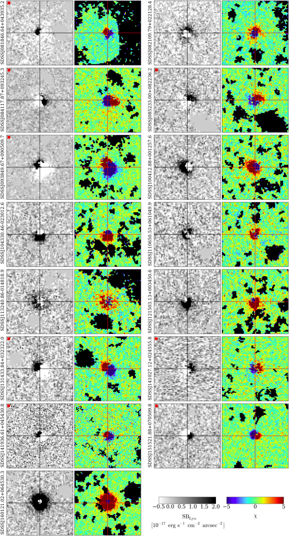
Figure 4.— Ly$\alpha$ surface brightness maps (linear-scale) and $\chi$-images (linear-scale) of 20″$\times$20″ (corresponding to about $164$ kpc $\times 164$ kpc at $z=2.253$) after continuum and PSF subtraction centered on each quasar of our sample. The position of the peak of the quasar before PSF subtraction is indicated by the cross. The PSF subtraction reveals Ly$\alpha$ emission above SB${}_{{\rm Ly}\alpha}=10^{-17}$ erg s^-1 cm^-2 arcsec^-2 extending on scales of radius $\sim 3-4$ arcsec ($\sim 25-32$ kpc) around 7 out of 15 quasars, i.e. 47% of the sample. The quasars whose PSF subtraction reveal stronger residuals are indicated with a red square in the top-left corner of their image. North is up, East is to the left.

3.3. Constraining the PSF of the NB Images

To quantify the extended emission in the Ly$\alpha$ line around the quasars in our fields, i.e. not related to unresolved emission from the quasar itself, we have to carefully estimate the PSF of our NB images. We need to compute the PSF with high accuracy, in order to detect even small deviations from its shape in the average profile of the QSOs. For this purpose, we match the SDSS star catalogue with the sources in our 15 NB fields and select all the high S/N stars. This operation resulted in a sample of 115 usable stars. For each of these stars, we have created the NB masked image as explained in §3.1, and calculated the stars emission profile in radial logarithmic bins (see red circles in Figure 2) with an unweighted average of all the not-masked pixels within each annulus. We then consistently propagate the errors from the variance image. The profiles of the 115 stars are then averaged with equal weights to obtain the PSF of the NB images.

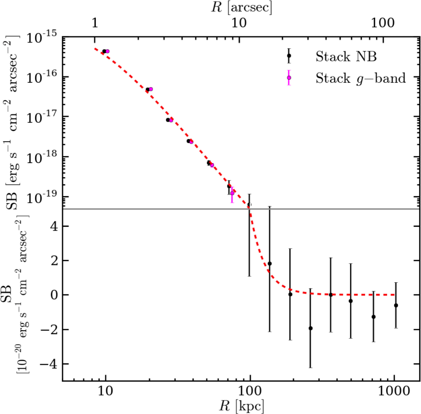
Figure 5.— Average radial profile for 115 stars in our NB images (black points). This PSF is well fitted by a Moffat profile with FWHM$=1.2$″, and $\beta=2.15$ (red dashed line). Note the different scale in the plot, i.e. log-log plot to capture the whole range of the PSF, and log-linear to check the zero level at large radii. The PSF of the NB images (black) is in good agreement with the PSF of the $g$-band (magenta). Note that the $g$-band data points have been normalized to the NB observations (see text for details), and artificially moved at slightly higher radii to avoid superposition with the NB data points.

Figure 5 shows the average radial profile for the 115 high S/N stars in our NB images (black points). The profile is consistent with a Moffat function, as expected for seeing limited observations, where the PSF is determined by the wiggling of the stars on the CCD (Trujillo et al. 2001). The normalized Moffat profile is defined as

$${\rm PSF}(r)=\frac{\beta-1}{\pi\alpha^{2}}\left[1+\left(\frac{r}{\alpha}\right)^{2}\right]^{-\beta},$$ (3)

where the full width at half maximum is given by FWHM$=2\alpha\sqrt{(2^{1/\beta}-1)}$, and the total flux is normalized to 1. We fit the average profile of the stars with this function and obtained best fit parameter values of FWHM=1.2″and $\beta=2.15$. The FWHM value we obtained is perfectly consistent with the independent measurement of the median seeing in our observations (see §2) estimated by selecting all the stars in the images, and applying the psfmeasure task within the IRAF software package. In the absence of imperfections in telescope optics, the $\beta$ parameter in eqn. (3) should have a value of $\sim 4.765$, as expected from turbulence theory (e.g., Saglia et al. 1993; Trujillo et al. 2001). However, it is known that PSFs typically measured in real images have larger “wings”, or equivalently, smaller values of $\beta$. This is due to the fact that the real seeing also depends on the performance of the telescope optics, and not only on the atmospheric conditions (Trujillo et al. 2001). Our value is in agreement with this picture, however there is no tabulated PSF for the GMOS-S instrument (German Gimeno, private communication).

To test our PSF estimate, we perform the same calculation on masked $g$-band images. We select 15 high S/N not saturated stars, i.e. one per field to include in our calculation all possible seeing variations between different stacks. We then calculate the average radial profile, as for the stars in the NB images. Figure 5 shows (in magenta) this average radial profile after normalizing it to the NB data points. The normalization factor is computed as the ratio between the peak values of the two average profiles. The shape of the Moffat profile of the NB and $g$-band images are in remarkable agreement. Note that in the case of the $g$-band PSF calculation, we probe only smaller radii, due to confusion arising mainly from diffuse light from bright objects. Finally, note that the Moffat profile goes smoothly to zero at large radii, and the average star profile is consistent with this within our uncertainties (see log-linear region of the plot in Fig. 5).

Having characterized the PSF of our observations, we can now ascertain whether our sample of QSOs exhibit a signal from the surrounding diffuse gas distribution. To do so, we apply the same stacking analysis to the quasar sample.

4. Results

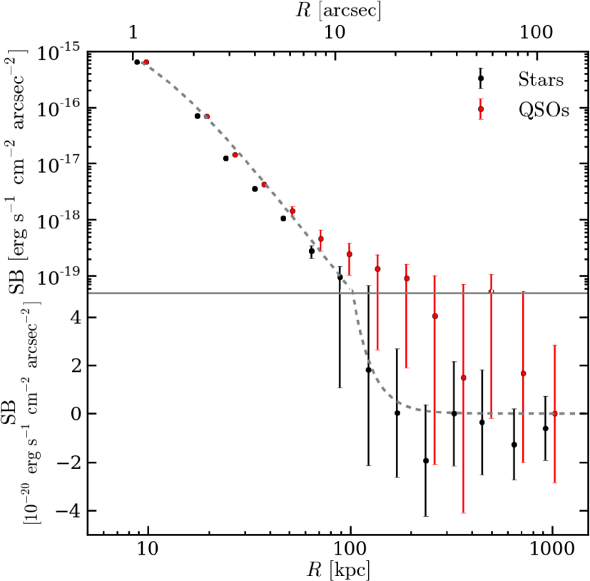
Figure 6.— Average radial profile of 15 QSOs compared to the average star profile normalized to the QSO data points. The plot is divided into a log-log plot to show the whole range of the profiles, and a lin-log plot showing that the QSOs’ profile is also consistent with zero at large radii. The gray dashed line indicate the Moffat profile with parameters derived from the fit to the stars’ profile. The QSOs’ profile shows a deviation from the stars’ PSF at SB $\sim 10^{-19}$ erg s^-1 cm^-2 arcsec^-2. The stars’ profile is slightly shifted to smaller radii for clarity (e.g. to avoid the superposition of the errorbars).

As done for the stars, we have computed the radial profile for each quasar from the NB masked images. The 15 quasar profiles are then averaged to obtain the average signal around $z=2.253$ quasars. Figure 6 shows the average radial profile of the QSOs, together with the average profile of the stars normalized to the QSOs data points. The normalization has been performed by multiplying the average star profile by the ratio between the peak values of the two average profiles, i.e. the first bin. As the first annulus for the profile extraction has a radius of 1.2″  this is also consistent with an approximate normalization in flux. In addition, for comparison purposes, in this plot we slightly shift the stars’ PSF profile to smaller radii, i.e. the profiles are estimated with the same radial bins, but are shown at different locations to avoid the overlap of the error-bars. The QSOs’ profile clearly deviates from a pure Moffat function at large radii ($\gtrsim 70$ kpc), and at a low surface brightness level of SB$\sim 10^{-19}$ erg s^-1 cm^-2 arcsec^-2, and, as expected, is consistent with zero at very large radii ($\gtrsim 600$ kpc).

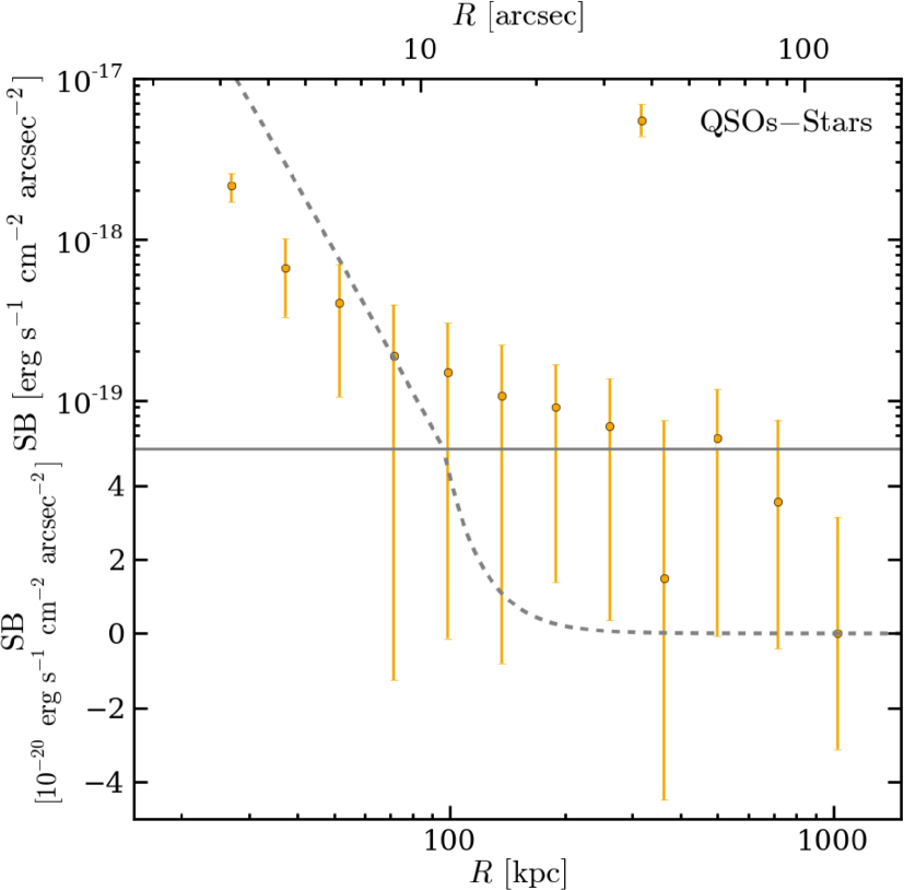
Figure 7.— Difference of the average QSO profile and the normalized stars profile. This may be interpreted as the average SB_Lyα profile from the gas distribution around a typical $z\sim 2$ QSO. Note the extremely low surface brightness probed at large distances from the quasars.

This extended emission is more evident if we take the difference between the QSOs’ profile and the normalized stars’ profile, or in other words, if we remove the contribution from the unresolved emission of the QSOs. The resulting profile thus represents the average Ly$\alpha$ emission arising from the distribution of the cool gas (${T\sim 10^{4}}$ K) around a typical bright $z\sim 2$ QSO. Figure 7 displays the profile of the difference between QSOs and the normalized star profile, which extends for hundreds of kpc to very low SB levels SB${}_{\rm Ly\alpha}\sim 10^{-19}-10^{-20}$ erg s^-1 cm^-2 arcsec^-2. However, we stress again that we do not subtract the continuum emission from the NB images and thus, on small scales, i.e. the scale of the quasar’s host (tens of kpc), the signal we see might be due to contamination from the resolved host galaxy or is emitted within the aforementioned EELR. If this is due to the host galaxy, we estimated from our profile that the galaxy should have $f_{\lambda}=2.03\times 10^{-17}$ erg s^-1 cm^-2 Å^-1 within an aperture of 3 arcsec radius ($\sim 25$ kpc), or equivalently a magnitude of 23.9. This value is similar to the rest-frame UV apparent magnitude of a bright Lyman break galaxy (LBG) at comparable redshift (e.g., Reddy & Steidel 2009), and thus brighter than a $L_{\star}$ galaxy for LBGs, i.e. $m_{\star}=24.54$ ($R_{\rm AB}$; Adelberger & Steidel 2000).

In addition, we check if the signal we detect is dominated by a single bright object in the stack by repeating the same experiment each time removing a different QSO from our sample. Specifically, we compute 15 average profiles of 14 QSOs, each time removing a different QSO. Then, to obtain the CGM profiles, we subtract from each of them the normalized star profile. In this way, it would be clear if a bright QSO in our sample dominates the stack at any radius.

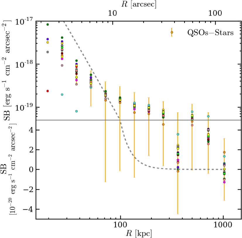
Figure 8.— Dependence of the Ly$\alpha$ profile on each individual QSO. We estimate the difference between the QSOs’ profile and the normalized stars’ profile 15 times, each time by removing a different QSO from the QSOs’ profile calculation. The different profiles are shown with different colors. It is clear, that none of the QSOs of the sample is dominating the Ly$\alpha$ profile for $R>50$ kpc. Larger variations, i.e. larger than the $1\sigma$ error, occur at smaller radii. This is probably due to slightly different seeing variations or host galaxy contamination (see §4).

Figure 8 shows the results of this test. It is clear that the profile is not changing significantly between different calculations for $R>50$ kpc. For smaller radii, as explained above, differences could arise due to seeing variations or host galaxy contamination. However, this is not the focus of the current work, and we are confident that none of the QSOs in our sample dominates the average profile on the large scales $R>50$ kpc characteristic of the CGM. However, given that the signal is close to our detection limit we verify the significance of our results in the next section.

4.1. Testing the Significance of the Results with a Monte Carlo Analysis

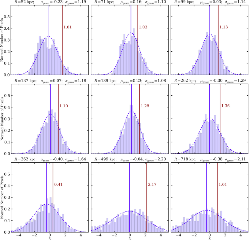
Figure 9.— $\chi$ histograms of the 1000 realizations of our same experiment (see Section for details) using random samples of 15 stars each. We show the histograms for each bin starting from $\sim 50$ kpc. The histograms are consistent with Gaussian distributions centered in zero (see the central $\mu_{\rm gauss}$ values) and with nearly unit variance (see the $\sigma_{\rm gauss}$ values) till $\sim 300$ kpc. The bins at larger radii seem to deviate from the simple Poisson statistics. The blue vertical lines indicate the central value of each histogram ($\mu_{\rm gauss}$), while the vertical brown lines indicate the $\chi$ for our measurements in Fig. 7.

Given the faintness of the emission we are looking for, we have applied an ad-hoc complicated preparation of our images before the profile extraction. Although this effort suggests a tentative detection, our results could still be dominated by systematic errors. In particular, our measurement of the CGM radial profile out to very large radii could be affected by 1) errors in the empirical PSF subtraction of the quasar profile using the PSF of stars, including errors in the re-scaling of the stellar PSF; and 2) systematics in the data reduction and in the data itself (e.g., flat-fielding, constant sky-subtraction, ccd-noise, masking). These systematics could prevent the noise from averaging down according to simple photon-counting statistics, i.e. the expected error on the average SB should be inversely proportional to the square root of the area employed in the average ${\sigma_{\rm SB}^{\rm Area}=\sigma_{\rm SB}^{\rm 1arcsec^{2}}/\sqrt{\rm Area}}$.

For these reasons, to firmly assess the statistical significance of our results, we perform a Monte Carlo analysis. We have built $1000$ samples of 15 stars, by randomly selecting objects from the 115 stars that were used to determine the PSF of the NB images (see §3.3). For each sample of stars we have then computed the average radial profile, and subtracted from it the normalized average profile of the global sample of the stars. In this way, we are left with $1000$ realizations of our same experiment, i.e. QSOs’ profile $-$ stars’ profile. These profiles should be consistent with zero at each radius, and the $\chi$ values, i.e. the ratio between the signal and the 1$\sigma$ error within each bin, should be consistent with a Gaussian distribution of unit variance. If however we find Gaussian distributions with variances greater than 1, this would give us information on the degree to which we are underestimating the noise, and/or at which radius systematics begin to dominate the error budget. Furthermore, these Monte Carlo simulations of the null experiment will allow us to robustly estimate the statistical significance of our detection in a way that also folds in both the formal statistical errors, as well as the systematic errors.

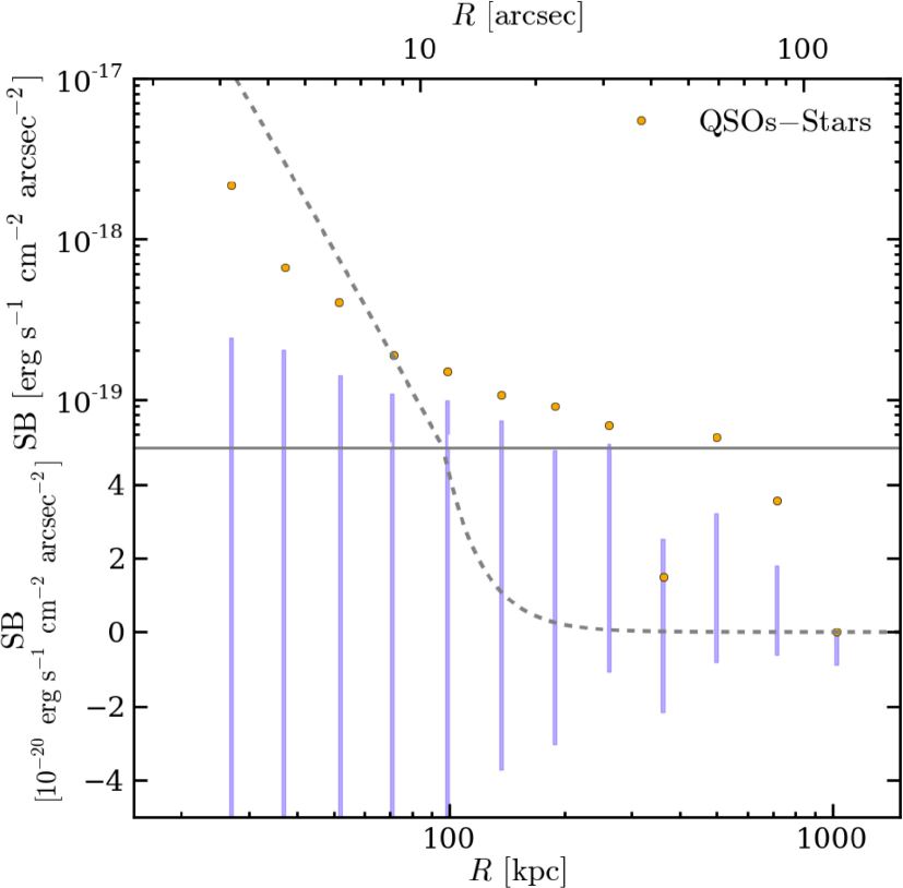
Figure 10.— The difference between the QSOs’ profile and the average profile of the 115 stars (yellow) is compared with the confidence area within the 16th and the 84th percentiles from the Monte Carlo analysis (blue shaded area). Using the current radial bins, there is only a hint for Ly$\alpha$ signal, as already clear from Fig. 9.

In Figure 9 we show the distribution of the $\chi$ values for these 1000 realizations in each radial bin, starting from the $\sim 50$ kpc radius, and compare them to our results. We focus on the histograms for the larger radii because, as discussed in the previous section, the smaller scales can be contaminated by EELR or host galaxy emission which are not the focus of the current study. It is clear that the histograms have an approximately Gaussian shape, well centered on zero (blue vertical lines). However the variances increase at large radii, indicating that the error budget is deviating from the expectation based on photon counting statistics. Indeed, for ${R\lesssim 200}$ kpc, we only slightly underestimate the noise (by $\sim 15$%), while at larger radii we incur significantly larger errors than photon counting would suggest. This is likely due to the fact that bins at larger radii, i.e. $\gtrsim 400$ kpc, probe larger area and the implied SB limit is significantly lower. As our SB limit decreases we become more sensitive to subtle systematics in the data, e.g. correlations between neighboring pixels, which are larger than the formal photon counting error, and which may not average down as $\sqrt{\rm Area}$. As we noted at the beginning of this section, this deviation can be ascribed to several possible effects.

The brown vertical lines in Figure 9 indicate the measurements obtained in the previous section for comparison (Figure 7). Note that all our measurements constitute a positive fluctuation which is not expected for a spurious signal. In other words, the Monte Carlo realizations are well centered around zero, while our measurements always exhibit positive values. Given the current binning, with the exception of the bin at 362 kpc, we have a $>1\sigma$ fluctuation in every bin (or in other words above the 84th percentile of the Monte-Carlo realizations).

This can be better visualized in Figure 10, where we highlight the area within the 16th and 84th percentile of the 1000 realizations in comparison to the difference profile between QSOs and stars, e.g. same profile of Figure 7. Note that in agreement with the previous histograms (Fig. 9), the 16th percentile of the 1000 realizations is negative. This can be seen in the log-lin part of Figure 10. Note however that our Monte-Carlo realizations are not well centered around zero following the uncertainties expected in some of the annuli, i.e. the error on the mean should be given by $\sigma_{\rm gauss}/\sqrt{1000}$ and thus fluctuations of our mean values about zero should be comparable to this. In other words, we stress that the presence of systematics also appears to give rise to larger fluctuations about zero in our Monte-Carlo realizations than simple Gaussian statistics would suggest. However, it is reassuring that these fluctuations are nevertheless both positive and negative and do not show up in all annuli.

Further, although the statistical significance in a single radial bin is not high, we can combine our data to increase the signal-to-noise ratio of our detection. We decide to consider the data in one large radial bin spanning from $50$ kpc $<R<500$ kpc, and conduct a similar Monte Carlo analysis. Figure 11 shows the $\chi$ histogram of the 1000 realizations in comparison to our measurement (red vertical line) of the stacked PSF subtracted emission (i.e. QSO-star) for this large radial bin. As expected from the previous analysis, the distribution is clearly Gaussian and centered at zero, and we somewhat underestimate the error. Specifically, given that we find $\sigma_{\rm gauss}=1.30$, our error is underestimated by 30%. Taking this into account, the deviation of our measurement ($\sim 3\sigma$) from the distribution would correspond to a $2.32\sigma$ detection in this wide bin, or in other words, it falls in the 98.5th percentile of the Monte-Carlo realizations.

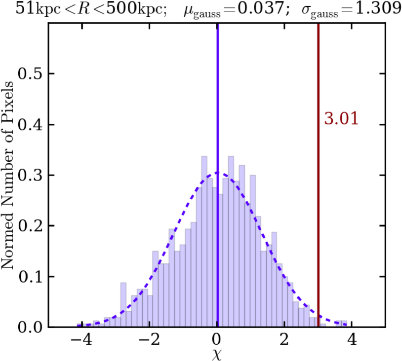
Figure 11.— $\chi$ histogram of the 1000 realizations of our same experiment using random samples of 15 stars each (see text for details) in a bin extending from $50$ kpc to $500$ kpc. The red vertical line indicates the $\chi$ value for our measurement in the same bin.

This detection corresponds to SB${}_{\rm Ly\alpha}=(5.5\pm 3.1)\times 10^{-20}$ erg s^-1 cm^-2 arcsec^-2 within an annular region extending from $50$ kpc to $500$ kpc around the QSO. In the next section we will discuss the implications of this measurement in the context of our current understanding of the gas distribution around QSOs, both from observations and from simulations.

5. Discussion

As discussed in detail in the literature, given the resonant nature of the Ly$\alpha$ line one needs to be particularly cautious when interpreting observations of this emission (e.g., Gould & Weinberg 1996; Cantalupo et al. 2005; Dijkstra et al. 2006; Verhamme et al. 2006). Further, as summarized in the introduction, multiple physical processes can potentially power extended Ly$\alpha$ emission and disentangling them is challenging, especially given that several of them could be at work. These mechanisms are (i) resonant scattering of Ly$\alpha$ line photons (Dijkstra & Loeb 2008; Steidel et al. 2011; Hayes et al. 2011), (ii) photoionization by stars or by a central AGN (Geach et al. 2009; Overzier et al. 2013), (iii) cooling radiation from cold-mode accretion (e.g., Fardal et al. 2001; Yang et al. 2006; Faucher-Giguère et al. 2010; Rosdahl & Blaizot 2012), and (iv) shock-heated gas by galactic superwinds (Taniguchi et al. 2001; Dijkstra & Kramer 2012).

In the following discussion we assume that the dominant mechanism powering the faint Ly$\alpha$ emission we observed around quasars is photoionization from the central AGN, resulting in a boosted Ly$\alpha$ fluorescence signal from the surrounding gas distribution. Indeed, scattering of Ly$\alpha$ photons from the quasar should not be a major contributor on such large scales ($>100$ kpc, Cantalupo et al. 2014). This is because the resonant scattering process results in very efficient diffusion in velocity space, such that the vast majority of resonantly scattered photons produced by the quasar itself (or by the central galaxy) escape the system at very small scales ($<10$ kpc), and hence do not propagate to larger distances (e.g., Dijkstra et al. 2006; Verhamme et al. 2006; Cantalupo et al. 2005; Arrigoni Battaia et al. 2015a). Further, in the case of Ly$\alpha$ emission in a superwind we would expect much higher values than observed for the Ly$\alpha$ surface brightness, i.e. at least SB${}_{\rm Lya}\sim 10^{-18}$ erg s^-1 cm^-2 arcsec^-2 (Taniguchi et al. 2001), depending on shock velocity. However, we cannot rule out a cooling radiation scenario, and indeed, it is interesting to note that the SB_Lyα that we measure seems consistent with the SB values shown for massive halos at large radii ($\gtrsim 100$ kpc) by Rosdahl & Blaizot (2012), even though their simulations were run to interpret the LAB phenomenon and do not include the presence of an active AGN. Despite this, they predict much higher emission (SB${}_{\rm Lya}\sim 10^{-18}$ erg s^-1 cm^-2 arcsec^-2) at smaller scales ($R<100$ kpc) than we observe. Modeling the expected Ly$\alpha$ SB from cooling radiation clearly requires further detailed investigation.

We thus interpret the extended emission that we measured as AGN boosted Ly$\alpha$ fluorescence, and adopt two different approaches for our analysis. First, we consider the observed SB_Lyα in the context of the simple model for cool halo gas described in Hennawi & Prochaska (2013) (already used in Arrigoni Battaia et al. 2015a), combined with recent observational constraints on the cool gas distribution around $z\sim 2$ QSOs deduced from absorption line studies. Second, we compare our emission measurement to the results of a cosmological hydrodynamical simulation post-processed with ionizing and Ly$\alpha$ radiative transfer, which was run to interpret the UM 287 nebula (see Cantalupo et al. 2014).

By studying absorption features in the spectra of projected quasar pairs, the “Quasars Probing Quasars” series of papers (QPQ; Hennawi et al. 2006 and references thereafter) has shown that the optically thick absorbers arising from gas clouds within the halo of quasars are anisotropically distributed with respect to the quasar itself (Hennawi & Prochaska 2007). In other words, a quasar emits radiation anisotropically or intermittently, so that the number of optically thick absorption systems is higher in the background sightlines (i.e. at a certain projected distance from the quasar) in comparison to that observed along the line-of-sight to that quasar. This result, together with the absence of fluorescent emission from these optically thick absorbers (Hennawi & Prochaska 2013) as well as photoionization modeling of individual absorbers (Prochaska & Hennawi 2009; Lau et al. 2015) all indicate a scenario in which the optically thick gas observed in absorption toward background sightlines is shadowed from the ionizing radiation of the quasar. Prochaska et al. (2013b) have shown that these optically thick absorbers have a high covering factor $f_{\rm C}^{\rm thick}\simeq 0.6$ on $R\lesssim 200$ kpc in the quasar’s CGM (see also Hennawi & Prochaska, 2007; Prochaska et al., 2013a; Hennawi & Prochaska, 2013).

Hennawi & Prochaska (2013) argued that, given this high covering factor and the luminosity of the quasar, the optically thick clouds observed in absorption would result in a very bright signal if directly illuminated by the ionizing radiation of the quasar. We can estimate this SB for our sample assuming the simple model in Hennawi & Prochaska (2013), where a quasar is surrounded by a spherical halo populated with spherical clouds of cool gas ($T\sim 10^{4}$ K) at a single uniform hydrogen volume density $n_{\rm H}$, which are uniformly distributed throughout the halo, with an aggregate covering factor of $f_{\rm c}$. By assuming this model, the Ly$\alpha$ surface brightness for an optically thick distribution of clouds is given by (Hennawi & Prochaska 2013)

$${\rm SB}_{{\rm Ly}\alpha}^{\rm thick} = 6.7\times 10^{-17}\left(\frac{1+z}{3.253}\right)^{-4}\!\!\left(\frac{f_{\rm C}^{\rm thick}}{0.5}\right)\!\!\left(\frac{R}{160\,{\rm kpc}}\right)^{-2}$$

$$\times \left(\frac{L_{\nu_{\rm LL}}}{10^{30.9}\,{\rm erg\,s^{-1}\,Hz^{-1}}}\right){\rm\,erg\,s^{-1}\,cm^{-2}\,arcsec^{-2}}.$$

where we used the redshift of our observations ($z=2.253$), the virial radius of the dark matter halo hosting quasar as distance ($R=160$ kpc), and the specific luminosity at the Lyman limit (${{\rm log}\,L_{\nu_{\rm LL}}=30.9}$) corresponding to the average magnitude of our sample, i.e. $i$-mag $=18.64$. This value of $L_{\nu_{\rm LL}}$ is obtained as in Arrigoni Battaia et al. (2015a) by integrating the Lusso et al. (2015) composite quasar spectrum against the SDSS filter curve, and choosing the normalization which gives the correct magnitude for each quasar in our sample. This signal is almost three orders of magnitude larger than the observed SB value of the Ly$\alpha$ emission at 160 kpc from our stacking analysis, i.e. SB${}_{\rm Ly\alpha}\sim 10^{-19}$ erg s^-1 cm^-2 arcsec^-2, and would have been easily detected even in our individual exposures. Along the lines of the argument in Hennawi & Prochaska (2013), we conclude that the low SB signal that we observed cannot be arising from optically thick gas clouds illuminated by the quasar.

On the other hand, if we assume that gas with physical properties similar to the gas probed by absorption studies is uniformly distributed throughout the halo, the quasar would shine on the remaining $f_{\rm C}^{\rm thin}\simeq 1-f_{\rm C}^{\rm thick}$ component, keeping it highly ionized, i.e. optically thin. Following Hennawi & Prochaska (2013), we can thus show that such optically thin clouds would result in a Ly$\alpha$ SB level comparable to our observations

$${\rm SB}_{{\rm Ly}\alpha}^{\rm thin} = 8.8\times 10^{-20}\left(\frac{1+z}{3.253}\right)^{-4}\!\!\left(\frac{n_{\rm H}}{0.01\,{\rm cm^{-3}}}\right)$$

$$\times \left(\frac{f_{\rm C}^{\rm thin}}{0.5}\right)\!\!\left(\frac{N_{\rm H}}{10^{20.5}\,{\rm cm^{-2}}}\right){\rm\,erg\,s^{-1}\,cm^{-2}\,arcsec^{-2}},$$

where we used the redshift of our observations ($z=2.253$), the median value for the column density $N_{\rm H}$ found in absorption studies (Lau et al. 2015) and an expected value for the volume density $n_{\rm H}$ from simulation on such scales (e.g. 160 kpc; Rosdahl & Blaizot 2012).

Following the foregoing discussion, it is thus plausible that the low Ly$\alpha$ signal that we detect in our observations is due to optically thin gas illuminated by the quasars. Indeed, the only way to match our observations via emission from optically thick clouds would be to require a very low covering factor in eqn. (5), i.e. $f_{\rm C}^{\rm thick}\sim 0.001$, but this would be clearly in conflict with the results in Prochaska et al. (2013b), arguing for the optically thin scenario. Note that optically thin emission is also in agreement with our previous work on giant Ly$\alpha$ nebulae. Indeed, although the quasars in our sample are on average fainter (average $i$-mag=18.64) than the UM 287 quasar ($i$-mag=17.28, Cantalupo et al. 2014), Hennawi et al. (2015) show that the $z\sim 2$ quasar SDSSJ0841+3921 ($i$-mag=19.35), which is fainter than our average quasar, is able to keep the gas highly ionized and optically thin out to scales of a few hundred kpc. Specifically, SDSSJ0841+3921 is surrounded by a large scale ($\sim 300$ kpc) Ly$\alpha$ nebulosity which is as bright (SB${}_{\rm Ly\alpha}=1.3\times 10^{-17}$ erg s^-1 cm^-2 arcsec^-2) as that surrounding the UM 287 quasar (SB${}_{\rm Ly\alpha}=1.2\times 10^{-17}$ erg s^-1 cm^-2 arcsec^-2) . Similar to UM 287, this Ly$\alpha$ nebula is believed to result from fluorescent emission powered by the ionizing radiation of the QSO. Thus, the comparable SB_Lyα in these two distinct cases, together with the factor of $\sim 20$ difference in the quasar ionizing luminosity, strongly suggests that brightness of the central source does not play an important role, provided it is bright enough to ionize the surrounding gas distribution. This again favors an optically thin emission scenario, since in this regime eqn. (5) shows that the Ly$\alpha$ SB scales as SB${}_{\rm Ly\alpha}\propto f_{\rm C}^{\rm thin}N_{\rm H}n_{\rm H}$, which is independent of the luminosity of the quasar.

Having established that the optically thin regime is a good hypothesis, we can now derive the physical properties of the emitting gas. To break the degeneracy between the covering factor $f_{\rm C}^{\rm thin}$, column density $N_{\rm H}$, and volume density $n_{\rm H}$ intrinsic of our SB_Lyα measurement in the optically thin regime, we need independent constraints. Regarding $f_{\rm C}^{\rm thin}$, it has been shown that the smooth morphology of the emission in giant Ly$\alpha$ nebulae implies a covering factor of $f_{\rm C}^{\rm thin}\gtrsim 0.5$ (Arrigoni Battaia et al. 2015a, b; Hennawi et al. 2015). For simplicity, in what follows, we will always assume a covering factor of $f_{\rm C}^{\rm thin}=0.5$. Note that, as said before we are assuming $f_{\rm C}^{\rm thin}\simeq 1-f_{\rm C}^{\rm thick}$ , and thus this value is also well motivated by the distribution of optically thick absorbers, which show a high covering factor in the quasar’s CGM (Prochaska et al. 2013b).

Further, the total hydrogen column density $N_{\rm H}$ can be constrained via photoionization modeling of absorption systems along the sightlines of background QSOs that pierce through the halo of a foreground QSO (Lau et al. 2015 and references therein). In particular, Lau et al. (2015) compared photoionization models to a statistical sample of absorbers in the CGM of typical $z\sim 2$ QSOs, finding a median ${{\rm log}\,N_{\rm H}=20.5}$ within $200$ kpc from the quasars, although they observed a substantial scatter in the distribution of $N_{\rm H}$ values, i.e. $\sim 1.5$ dex (see Fig. 15 of Lau et al. 2015). A similar value ${{\rm log}\,N_{\rm H}=20.4\pm 0.4}$ (at impact parameter of $\sim 180$ kpc) was estimated from photoionization modeling of SDSSJ0841+3921, exploiting the so far unique case where a giant Ly$\alpha$ nebula could be modeled in both emission and absorption (Hennawi et al. 2015). Given that these are the most recent and reliable estimates for $N_{\rm H}$ in the literature which are also consistent with each other, we henceforth assume a value of ${{\rm log}\,N_{\rm H}=20.5}$ throughout our analysis.

Thus plugging in the values $z=2.253$, $f_{\rm C}=0.5$, and ${{\rm log}\,N_{\rm H}=20.5}$ into eqn. (5), for the Ly$\alpha$ SB in the optically thin scenario, we find the typical volume density $n_{\rm H}$ expected on scales of ${\sim 275}$ kpc , given that SB${{}_{\rm Ly\alpha}=(5.5\pm 1.8)\times 10^{-20}}$ erg s^-1 cm^-2 arcsec^-2 from our measurement. We thus obtain an estimate of the volume density of the gas illuminated by the quasar and fluorescing in Ly$\alpha$:

$$n_{\rm H} = 0.6\times 10^{-2}\left(\frac{{\rm SB}_{{\rm Ly}\alpha}^{\rm thin}}{5.5\times 10^{-20}{\rm\,erg\,s^{-1}\,cm^{-2}\,arcsec^{-2}}}\right)$$ (6)

$$\times \left(\frac{f_{\rm C}}{0.5}\right)^{-1}\left(\frac{N_{\rm H}}{10^{20.5}\,{\rm cm^{-2}}}\right)^{-1}\,{\rm cm}^{-3}.$$

Given this estimate for $n_{\rm H}$ at $R=275$ kpc, we can compute the ionization parameter $U\equiv\Phi_{LL}/cn_{\rm H}\propto L_{\nu_{\rm LL}}/n_{\rm H}$ at these distances around quasars. If we assume that $n_{\rm H}$ is not affected by illumination on these large scales, its value holds for both the shadowed and illuminated gas, and $U$ varies due to the different ionizing sources, either the ultraviolet background (UVB; e.g., Haardt & Madau 2012) if the gas is shadowed from the quasar emission, or the quasar if it is illuminated. We find a value of ${\rm log}\,U_{\rm UVB}=-3.2$ and ${\rm log}\,U_{\rm QSO}=-0.2$ for shadowed gas and illuminated gas, respectively. For randomly observed absorption systems, we thus expect to see a strongly bi-modal distribution of $U$ values. Hence, it is interesting to compare this result with what was found by Lau et al. (2015) from photoionization modeling of individual absorbers. Indeed photoionization modeling constrains the ionization parameter $U$, as long as ionic ratios can be measured (e.g. C⁺/C³⁺, Si⁺/Si³⁺). Note that the average ionizing luminosity of their sample is ${{\rm log}\,L_{\nu_{\rm LL}}=30.4}$, i.e. 0.5 dex lower than our sample, resulting in ${\rm log}\,U_{\rm QSO}=-0.7$.

In their data there is no sign for a bi-modal distribution in $U$ (see Figure 7 in Lau et al. 2015), with low ionization parameter ${\rm log}\,U\lesssim-2$ at any distance from the quasar and no systems at higher $U$, implying that these absorbers are likely not illuminated by the quasar. It is thus plausible that the Lau et al. sample was biased against sources with very high $U$ values, which would result in fewer detectable metal absorption lines needed to constrain the ionization parameter through photoionization models. Indeed, two systems out of 14 studied by Lau et al. (2015), i.e. J0409-0411 and J0341+0000, do not have metal line detections, and thus do not have constraints on the ionization state of the gas, i.e. no estimate on $U$. Nevertheless, the situation is more complicated with effects that can wash out the bi-modal distribution expected from the simple picture of half shadowed and half illuminated gas. In particular, star-forming galaxies in the vicinity of the absorber could boost the $U$ value of shadowed sources from $U_{\rm UVB}$ to a higher $U_{\rm local}$. Further, the real distance between QSO and absorber is unknown, i.e. we have information only on the projected distance on the sky. If the real distance is 2-3 times larger than the projected distance, this would result in a reduction of 4-10 in $\Phi_{LL}$, and hence in $U$. In addition, if the highly ionized gas has similar velocity as the less ionized gas, its absorption features would then be lost in the stronger absorption of the less ionized gas, resulting in a bias against such high-U absorption systems. Clearly, to confirm this scenario and test the relevance of these additional effects, further observations and analysis are needed.

However, given that we have an estimate for $U_{\rm QSO}$, it is then interesting to understand which kind of absorption features are expected from the gas that we detect here in emission and compare them to the two systems in Lau et al. (2015), which do not have metal line detections. To estimate this, we use the photoionization code Cloudy (Ferland et al. 2013) to calculate the column densities expected for different ions for an optically thin slab of gas at the distance of $R=275$ kpc from the quasar. As input parameters we used the aforementioned quantities that would give rise to the observed Ly$\alpha$ emission, i.e. $N_{\rm H}=10^{20.5}$ cm^-2, ${\rm log}\,U_{\rm QSO}=-0.2$. We have then included the presence of the ultraviolet background (UVB; Haardt & Madau 2012), and assumed the gas to have a metallicity of $Z=0.1$ Z_⊙, similar to values in Lau et al. (2015). This calculation shows that in the Ly$\alpha$ emitting gas $N_{\rm HI}=10^{14.9}$ cm^-2, $N_{\rm CIV}=10^{12.8}$ cm^-2, $N_{\rm NV}=10^{12.9}$ cm^-2, $N_{\rm OVI}=10^{14.9}$ cm^-2, and both $N_{\rm SiII}$ and $N_{\rm FeII}$ have very low values ($\ll 10^{10}$ cm^-2), confirming that would be extremely difficult to detect metal absorption from such systems. Indeed, the two highly ionized systems reported in Lau et al. (2015) have column densities comparable to these expectations. In particular, J0409-0411 shows $N_{\rm HI}=10^{14.2}$ cm^-2, $N_{\rm CIV}<10^{13.31}$ cm^-2, $N_{\rm SiII}<10^{13.48}$ cm^-2, and has an impact parameter of 190 kpc from the quasar, while J0341+0000 similarly shows $N_{\rm HI}=10^{14.2}$ cm^-2, $N_{\rm CIV}<10^{13.28}$ cm^-2, $N_{\rm SiII}<10^{13.42}$ cm^-2, $N_{\rm FeII}<10^{13.62}$ cm^-2, and has an impact parameter of 235 kpc. Thus, our analysis suggests that these two systems in Lau et al. (2015) are good candidates for background sightlines piercing gas which is illuminated by the quasar, and hence optically thin, and characterized by a high ionization parameter.

Lastly, we can compare our empirically derived $n_{\rm H}$ value with simulations. We are not aware of an average density profile for the cool gas in massive (M${}_{\rm DM}\sim 10^{12.5}$ M_⊙) halos in the literature, although we plan to determine it in future work. Simulations of massive halos (e.g., Rosdahl & Blaizot 2012) usually predict $n_{\rm H}$ values in the range ($\sim 10^{-2}-10^{-3}$ cm^-3) on these scales ($\sim 200$ kpc) within filamentary structures. These values are in rough agreement with our estimate. However, they may not optimally resolve this gas (Cantalupo et al. 2014; Crighton et al. 2015), and high densities are also probably present (Arrigoni Battaia et al. 2015a; Lau et al. 2015).

Cantalupo et al. (2014) showed that one can calibrate relations between SB_Lyα and the total hydrogen column density in cosmological simulations post-processed with radiative transfer using the RADAMESH Adaptive Mesh Refinement code (Cantalupo & Porciani 2011), resulting in a picture which is consistent with the simple analytical relations discussed above, i.e. eqn. (5) and eqn. (5). By comparing pixel by pixel the mock image obtained for the SB_Lyα and the $N_{\rm HII}$ column density map of cool gas ($T<5\times 10^{4}$ K) in the case where the gas is mostly ionized by the quasar, i.e. what we above referred to as the optically thin scenario, Cantalupo et al. (2014) obtained the following relation from their simulation:

$$N_{\rm HII}=10^{21}\,\left(\frac{{\rm SB_{\rm Ly\alpha}}}{10^{-18}\,{\rm erg\,s^{-1}\,cm^{-2}\,arcsec^{-2}}}\right)^{1/2}C^{-1/2}\,{\rm cm^{-2}}.$$ (7)

This relation depends on the clumping factor ${C=\langle n_{\rm H}^{2}\rangle/\langle n_{\rm H}\rangle^{2}}$, introduced by Cantalupo et al. (2014) to account for dense gas on small scales that are possibly unresolved by the simulation. If we plug in our value of SB${}_{\rm Ly\alpha}=5.5\times 10^{-20}$ erg s^-1 cm^-2 arcsec^-2, and assume $C=1$, we find ${{\rm log}\,N_{\rm H}=20.37}$, which is consistent with the simulation values (see Extended Data Fig. 3 of Cantalupo et al. 2014), and in agreement, within the uncertainties, to the observational value we used in the foregoing discussion ${{\rm log}\,N_{\rm H}=20.5}$. We thus find agreement between simulations and our simple analytical model in the case of these low SB levels, as opposed to the case of the giant bright Ly$\alpha$ nebulae, where very high clumping factors are required by simulations to match the observed SB_Lyα, with values up to $C\sim 1000$ (Cantalupo et al. 2014).

In summary, we argue that the hydrogen volume density around typical QSOs on $>100$ kpc scales is approximately constrained to be $n_{\rm H}\simeq 0.6\times 10^{-2}$ cm^-3, in broad agreement with the cool phase densities found in cosmological simulations . However, bright giant Ly$\alpha$ nebulae, like UM 287 (Cantalupo et al. 2014) and SDSSJ0841+3921 (Hennawi et al. 2015), appear to require much higher densities $n_{\rm H}\gtrsim 1$ cm^-3 (Cantalupo et al. 2014; Arrigoni Battaia et al. 2015a; Hennawi et al. 2015), to explain their higher SB Ly$\alpha$ emission. Thus our analysis indicates a scenario in which $\sim 10$% of quasars show bright giant Ly$\alpha$ nebulae (SB${}_{\rm Ly\alpha}\sim 10^{-17}$ erg s^-1 cm^-2 arcsec^-2 on scales $>50$ kpc) which require high gas densities, while the remainder of the population is characterized by fainter extended Ly$\alpha$ emission and thus by much lower gas densities. At the moment, it is not clear what physical process is responsible for these factor of $\sim 100$ difference in gas density. It has been argued that the presence of a giant Ly$\alpha$ nebula may be physically connected to the location of over-densities of galaxies and AGN which provides an important clue (Hennawi et al. 2015).

5.1. Comparison with Previous Deep Observations around Quasars

Although many studies have targeted extended emission around individual quasars (Hu & Cowie 1987; Heckman et al. 1991a, b; Christensen et al. 2006; Hennawi et al. 2009; North et al. 2012; Hennawi & Prochaska 2013; Roche et al. 2014; Herenz et al. 2015), they do not achieve the SB sensitivity indicated by our stacked profile of the quasar CGM. This is primarily due to the limited sensitivity of the instruments employed in these studies or because they had a different chief science goal, e.g. focused on studying the much brighter emission from the EELR on smaller scales (Christensen et al. 2006).

On the other hand, both Rauch et al. (2008) and Cantalupo et al. (2012) have targeted quasars down to interesting sensitivity levels that should, according to our average profile, allow one to detect emission on 100 kpc scales. In particular, Rauch et al. (2008) achieve a SB limit of SB${{}_{\rm Ly\alpha}=8\times 10^{-20}}$ erg s^-1 cm^-2 arcsec^-2 ($1\sigma$ in 1 arcsec²) in their 92 h long-slit observations of the quasar DMS 2139-0405 ($z=3.2$; Hall et al. 1996), while Cantalupo et al. (2012) reach SB${{}_{\rm Ly\alpha}\sim 4\times 10^{-19}}$ erg s^-1 cm^-2 arcsec^-2 ($1\sigma$ in 1 arcsec²) with 20 h of narrow-band imaging targeting the $z=2.4$ quasar HE0109-3518. Although these studies reached interesting depths, they do not appear to show evidence for any extended Ly$\alpha$ emission on large scales. However, as we have shown, probing these extremely low surface brightness levels on 100 kpc scales requires a very careful analysis with proper accounting of systematics (e.g., flat-fielding, sky and continuum subtraction, contamination from nearby sources) and a specifically tailored analysis. It would be interesting to search for the extremely faint CGM Ly$\alpha$ emission that we detected in our stack in these very deep observations of individual quasars, which we plan to pursue in future work.

5.2. Comparison with LBGs and LAEs Ly$\alpha$ Profiles

With the aim of comparing our newly determined Ly$\alpha$ profile with previous observations at comparable redshift, and to gain a better overview on extended Ly$\alpha$ halos, we compile extended Ly$\alpha$ profiles for different sources from the literature. The left panel of Figure 12 shows our data together with the average profile of 92 continuum-selected LBGs at $\langle z\rangle=2.65$ (dashed magenta line; Steidel et al. 2011), the average profile of 24 proto-cluster LBGs at $z\sim 3$ (brown squares; Matsuda et al. 2012), the average profile of 130 LAEs at $z\sim 3$, selected to be in dense regions $2.5<\delta_{\rm LAE}<5.5$ (blue squares; Matsuda et al. 2012), and the median profile of 27 faint line emitters at $2.66<z<3.75$ (cyan triangles; Rauch et al. 2008).

The origin of Ly$\alpha$ halos around these star-forming galaxies is still a matter of debate, and, as for the case of giant Ly$\alpha$ nebulae around quasar, several mechanisms have been discussed in the literature. First, it is important to point out that Ly$\alpha$ cooling radiation is not able to account for the high Ly$\alpha$ luminosity of these halos, i.e. $L_{\rm Ly\alpha}\gtrsim 10^{42}$ erg s^-1, giving rise to halos which are an order of magnitude fainter than observed (e.g., Haiman et al. 2000; Dijkstra & Loeb 2009; Dijkstra & Kramer 2012, but see also Rosdahl & Blaizot 2012). However, an additional boost to the Ly$\alpha$ emission could result from the ionizing photons emitted by the galaxy itself or by nearby galaxies (e.g., Dijkstra & Loeb 2009; Mas-Ribas & Dijkstra 2016). The photoionized gas could then emit enough Ly$\alpha$ photons to be consistent with the observations. This would depend, however, on the ionizing photon escape fraction. Further, resonant scattering is not able to reproduce the extent of the Ly$\alpha$ halo, giving rise to more compact emission than observed (e.g., Dijkstra & Kramer 2012; Lake et al. 2015), unless bipolar outflows in which the clumps decelerate (in the case of LBGs; Dijkstra & Kramer 2012), or additional sources of Ly$\alpha$ emission (in the case of LAEs; Lake et al. 2015), such as low star-formation spatially distributed inside the host dark matter halo or cooling radiation, are taken into account. In summary, current studies suggest that in the case of LAEs and LBGs, as it is the case for QSO, a strong contribution from photoionization is needed in order to explain the extent and surface brightness of the Ly$\alpha$ halo observed, with up to 50-60% of the observed Ly$\alpha$ signal due to this powering mechanism (Mas-Ribas & Dijkstra 2016).

In the right panel of Figure 12, we show the Ly$\alpha$ profile of the UM 287 nebula (red; Cantalupo et al. 2014) and of the Ly$\alpha$ nebula around SDSSJ0841+3921 (blue; Hennawi et al. 2015) that we have computed from the continuum-subtracted NB image by averaging in circular apertures around the QSO after masking all the sources from the $V$-band (i.e. available broad band) and compact sources from the NB, as done for our individual objects in the GMOS observations (see §3.1). Note that the data reduction of UM 287 and SDSSJ0841+3921 has been performed differently. First of all, the Ly$\alpha$ image has been obtained through a continuum-subtraction (see Cantalupo et al. 2014; Hennawi et al. 2015), and no empirical PSF-subtraction has been performed on these data. Further, no detailed variance images have been computed. For these reasons, the errors shown in this plot for UM 287 and SDSSJ0841+3921 do not include the errors on the continuum and PSF subtraction, but are instead estimated through a bootstrap analysis ($1\sigma$). Note that these profiles, as highlighted in our analysis, could be affected by systematics at large radii (i.e. $\gtrsim 200$ kpc), where imperfections in the data reduction and in the data itself may be dominant (e.g., flat-fielding, sky-subtraction, continuum subtraction). In both panels we indicate with a vertical line the expected virial radius for a QSO at this redshift ($R_{\rm vir}^{\rm QSO}\sim 160$ kpc, Prochaska et al. 2014). As stressed already in our previous work, the extent of the Ly$\alpha$ emission goes beyond the expected size of the dark matter halo hosting quasars.

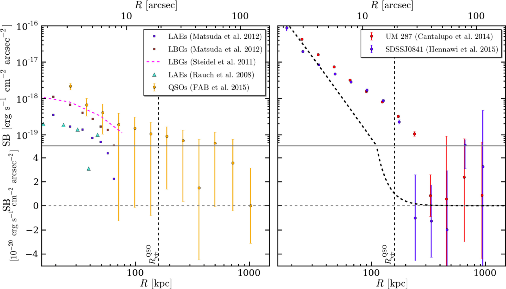
Figure 12.— Comparison of the extended Ly$\alpha$ surface brightness profiles for QSOs, LAEs, and LBGs. Left panel: We compare the profile already shown in Figure 7 with profiles reported in the literature: average profile of 92 continuum-selected LBGs at $\langle z\rangle=2.65$ (dashed magenta line; Steidel et al. 2011), average profile of 24 proto-cluster LBGs at $z\sim 3$ (brown squares; Matsuda et al. 2012), average profile of 130 LAEs at $z\sim 3$ (blue squares; Matsuda et al. 2012), median profile of 27 faint line emitters at $2.66<z<3.75$ (cyan triangles; Rauch et al. 2008). Right panel: We show the Ly$\alpha$ surface brightness profile for the giant nebulae around UM 287 (red; Cantalupo et al. 2014)and around SDSSJ0841+3921 (blue; Hennawi et al. 2015). Note that these two profiles are not PSF subtracted as in our stacking analysis. For this reason, we show a Moffat profile (black dashed curve) representing the seeing of the observations. In both panels, the vertical dashed line indicates the expected virial radius for a QSO at $z\sim 2$, i.e. $R_{\rm vir}^{\rm QSO}\sim 160$ kpc (Prochaska et al. 2014). Note that all QSO profiles (the one presented in this work, around UM 287 and SDSSJ0841+3921) have a signal of SB${}_{{\rm Ly}\alpha}\sim 10^{-19}$ erg s^-1 cm^-2 arcsec^-2 at 200 kpc.

Figure 12 shows that QSOs and LBGs have a higher emission profile which extends further out than LAEs. This could reflect the physics behind the Ly$\alpha$ emission, with objects able to ionize a larger amount of gas out to larger distances and characterized by a denser environment surrounded by higher and more extended Ly$\alpha$ signal. With the amount and distribution (density) of gas probably determining the strength of the Ly$\alpha$ emission (i.e. optically thin scenario), and with the environment probably determining the extent (Matsuda et al. 2012). In other words, this plot seems to suggest that more massive systems, i.e. the quasar population, show higher Ly$\alpha$ surface brightness profiles because the stronger ionizing radiation from the central source (or from nearby galaxies) is able to ionize the gas at much larger distances than in less massive systems. Indeed, ‘average’ LBGs and LAEs rely only on the ionizing radiation of stars (i.e. no bright QSO or AGN) and populate lower mass halos, i.e. $M_{\rm DM}\sim 10^{12}$ M_⊙ and $M_{\rm DM}\sim 10^{11}-10^{11.5}$ M_⊙ for LBGs and LAEs, respectively. Thus, probably for these reasons, their Ly$\alpha$ profile is lower and less extended.

On the other hand, systems like UM 287 and SDSSJ0841+3921 probably represent rare specific cases (i.e. $\sim 10$ % of quasars) where the gas densities are simply much higher. However, it is interesting to note that at $\sim 200$ kpc, both our stacked profile and the profiles for UM 287 and SDSSJ0841+3921 show a Ly$\alpha$ signal of SB${{}_{\rm Ly\alpha}\sim 10^{-19}}$ erg s^-1 cm^-2 arcsec^-2. It is thus plausible that our stacking analysis is consistent with (or detects) the same gas in the CGM or filamentary structures on these large scales around the quasars as for UM 287 and SDSSJ0841+3921 (Cantalupo et al. 2014; Arrigoni Battaia et al. 2015a; Hennawi et al. 2015). However, deep observations of a large sample of QSOs are needed to firmly characterize their extended Ly$\alpha$ profile with the same precision as for the LBGs and LAEs, and conclusions could be drawn only after disentangling the several mechanisms that can produce low SB Ly$\alpha$ emission.

6. Summary and Conclusions

Using NB imaging data collected as part of the FLASHLIGHT-GMOS survey (see also Arrigoni Battaia et al. 2013), we have performed a stacking analysis to characterize the extended Ly$\alpha$ emission around typical bright $z\sim 2$ QSOs. We find that:

• The 15 QSOs in our sample do not show giant Ly$\alpha$ nebulae similar to UM 287 (Cantalupo et al. 2014) or SDSSJ0841+3921 (Hennawi et al. 2015), i.e. SB${}_{{\rm Ly}\alpha}=10^{-17}$ erg s^-1 cm^-2 arcsec^-2 emission on scales $>50$ kpc, even though we would have been able to detect such emission. The PSF subtraction reveals Ly$\alpha$ emission above SB${}_{{\rm Ly}\alpha}=10^{-17}$ erg s^-1 cm^-2 arcsec^-2 extending on scales of radius $\sim 3-4$ arcsec ($\sim 25-32$ kpc) around 7 out of 15 quasars, i.e. 47% of the sample.

• The average radial profile of the 15 QSOs in our sample shows a deviation from the Moffat PSF of our NB images, starting at $\sim 70$ kpc at around SB${{}_{\rm Ly\alpha}\sim 10^{-19}}$ erg s^-1 cm^-2 arcsec^-2. This can be translated to a low significance first radial profile of the Ly$\alpha$ emission of the quasar CGM (see Figure 7). Using a Monte Carlo analysis (see §4.1), we ascertain that we have a $\sim 2.32\sigma$ detection within an annular bin spanning $50$ kpc $<R<500$ kpc from the QSOs. The Ly$\alpha$ emission in this bin, centered at $R=275$ kpc, is estimated to be SB${{}_{\rm Ly\alpha}=(5.5\pm 3.1)\times 10^{-20}}$ erg s^-1 cm^-2 arcsec^-2.

• Assuming a scenario in which the illuminated gas is highly ionized by the quasar radiation, the detected SB_Lyα on scales of hundreds of kpc implies gas volume densities of the order $n_{\rm H}=0.6\times 10^{-2}$ cm^-3. This value is much lower than what has been proposed in the case of extended bright Ly$\alpha$ nebulae around UM 287 (Arrigoni Battaia et al. 2015a) and SDSSJ0841+3921 (Hennawi et al. 2015), i.e. $n_{\rm H}\gtrsim 1$ cm^-3. However, our stacking analysis results in a Ly$\alpha$ profile consistent with the Ly$\alpha$ profile of UM 287 and SDSSJ0841+3921 on larger scales of $\sim 200$ kpc (SB${{}_{\rm Ly\alpha}\sim 10^{-19}}$ erg s^-1 cm^-2 arcsec^-2). Thus on these larger scales, it plausible that our stacking analysis detect a signal from the CGM or IGM as has been observed around UM 287 and SDSSJ0841+3921.

Future surveys targeting the Ly$\alpha$ line around QSOs with new IFU instruments, i.e. MUSE (Bacon et al. 2010) and KCWI (Morrissey et al. 2012), will be able to investigate the CGM of quasars without the tight restrictions on redshift range and redshift accuracy inherent in narrow-band imaging. This will allow one to observe a much broader range of quasars, enabling studies of quasars with specific attributes such as hyper-luminous quasars, obscured quasars, radio-loud quasars, or quasars in richer environments. Such studies are needed to test our current interpretation and to determine if specific types of quasar preferentially exhibit bright emission from their CGM.

Further, the lack of bright giant Ly$\alpha$ nebulae in our data confirm the necessity of large statistical samples of QSOs to uncover the brightest Ly$\alpha$ nebulae on the sky. The study of these bright nebulae, such as the UM 287 nebula (Cantalupo et al. 2014) or SDSSJ0841+3921 (Hennawi et al. 2015), enable further characterization of the CGM gas in individual systems via the detection and modeling of additional emission lines, e.g. C IV, He II (Arrigoni Battaia et al. 2015b, a). The resulting physical properties can then be used as additional constraints on simulations of galaxy-formation. Indeed, we call attention to the lack of high-resolution cosmological zoom simulations of very massive systems ($M_{\rm halo}\sim 10^{12.5}$ M_⊙) to which one could compare our results (but see Fumagalli et al. 2014 and Faucher-Giguere et al. 2016 for recent progress on this front). Given the complexity of the radiative transfer of the resonant Ly$\alpha$ line, simulations with both ionizing and Ly$\alpha$ radiative transfer of massive halos are needed to fully capture the physics in play in giant Ly$\alpha$ nebulae, and to compare to the wealth of observational data that are now becoming available.

Appendix A Estimate of the Flux Losses due to the Error on the Redshifts

As already stated in Section §2, the typical uncertainty on the redshift of our sample is $\sigma_{z}\sim 0.003$ (or equivalently $\sim 270$ km s^-1), which is much smaller than the width of the narrow-band filter used, i.e. $\Delta z=0.027$ (or equivalently $\Delta v=2479$ km s^-1). Further, to be sure that the Ly$\alpha$ emission of our targets fall within the narrow-band filter, we selected only QSOs whose redshift gives a maximum shift of $\pm 5$ Å from the filter’s center (or equivalently $\delta v=370$ km s^-1).

Nevertheless here, we test the robustness of our results against errors on the systemic redshift of the quasars in our sample. In particular, we estimate the flux losses due to this uncertainty. We proceed as follows. First, starting from the known systemic redshift of our sample, we build 1000 realizations of our 15 quasars by assuming that the error on the redshift is described by a gaussian distribution with $\sigma_{v}=300$ km s^-1, $750$ km s^-1, $1500$ km s^-1, or $3000$ km s^-1. Second, we assume that the signal we are looking for, i.e. the extended Ly$\alpha$ emission on scale of the CGM, is characterize by a ${\rm FWHM}=600$ km s^-1 centered at the systemic redshift of the quasar, as in the case of the giant nebula around UM 287 (Arrigoni Battaia et al. 2015a). Knowing the shape of our narrow-band filter, we are then able to compute the amount of flux lost for each sample of the 1000 realizations by taking the average of the loss per quasar within each sample.

Figure 13 shows the distribution of these average flux losses. This test shows that our sample should only be affected by a flux loss of the order of 3% (see blue histogram), while even doubling the error on the redshift would result in a 7% loss (green histogram). Only error distributions with width comparable to the width of our narrow-band filter can result in significant flux losses (see red and cyan histograms), and thus alter remarkably our analysis. Given the small uncertainty on the redshifts of our quasars, and our conservative selection criteria, we conclude that our sample do not suffer from flux losses.

Figure 13.— Estimate of the flux losses due to the error on the redshifts of our sample. Each histogram shows the distribution of the average flux loss for 1000 samples of 15 QSOs whose error on the redshift is assumed to be gaussian distributed with a $\sigma_{v}=300$ km s^-1 (blue), 750 km s^-1 (green), 1500 km s^-1 (red), or 3000 km s^-1 (cyan). Given that the errors on the redshift of our sample are of the order of 300 km s^-1, the flux losses do not affect our measurement.

References

- Adelberger & Steidel (2000) Adelberger, K. L., & Steidel, C. C. 2000, ApJ, 544, 218
- Alam & Miralda-Escudé (2002) Alam, S. M. K., & Miralda-Escudé, J. 2002, ApJ, 568, 576
- Arrigoni Battaia et al. (2013) Arrigoni Battaia, F., Hennawi, J. F., Cantalupo, S., & Prochaska, J. X. 2013, in Proceedings of the International Astronomical Union, Vol. 9, Multiwavelength AGN Surveys and Studies, 253–256
- Arrigoni Battaia et al. (2015a) Arrigoni Battaia, F., Hennawi, J. F., Prochaska, J. X., & Cantalupo, S. 2015a, ApJ, 809, 163
- Arrigoni Battaia et al. (2015b) Arrigoni Battaia, F., Yang, Y., Hennawi, J. F., et al. 2015b, ApJ, 804, 26
- Bacon et al. (2010) Bacon, R., Accardo, M., Adjali, L., et al. 2010, in Society of Photo-Optical Instrumentation Engineers (SPIE) Conference Series, Vol. 7735, Society of Photo-Optical Instrumentation Engineers (SPIE) Conference Series
- Bergeron et al. (2004) Bergeron, J., Petitjean, P., Aracil, B., et al. 2004, The Messenger, 118, 40
- Bertin (2006) Bertin, E. 2006, in Astronomical Society of the Pacific Conference Series, Vol. 351, Astronomical Data Analysis Software and Systems XV, ed. C. Gabriel, C. Arviset, D. Ponz, & S. Enrique, 112
- Bertin & Arnouts (1996) Bertin, E., & Arnouts, S. 1996, A&AS, 117, 393
- Binette et al. (1993) Binette, L., Wang, J. C. L., Zuo, L., & Magris, C. G. 1993, AJ, 105, 797
- Bowen et al. (2006) Bowen, D. V., Hennawi, J. F., Ménard, B., et al. 2006, ApJ, 645, L105
- Cantalupo et al. (2014) Cantalupo, S., Arrigoni-Battaia, F., Prochaska, J. X., Hennawi, J. F., & Madau, P. 2014, Nature, 506, 63
- Cantalupo et al. (2012) Cantalupo, S., Lilly, S. J., & Haehnelt, M. G. 2012, MNRAS, 425, 1992
- Cantalupo et al. (2007) Cantalupo, S., Lilly, S. J., & Porciani, C. 2007, ApJ, 657, 135
- Cantalupo & Porciani (2011) Cantalupo, S., & Porciani, C. 2011, MNRAS, 411, 1678
- Cantalupo et al. (2005) Cantalupo, S., Porciani, C., Lilly, S. J., & Miniati, F. 2005, ApJ, 628, 61
- Cen & Zheng (2013) Cen, R., & Zheng, Z. 2013, ApJ, 775, 112
- Charlot & Fall (1993) Charlot, S., & Fall, S. M. 1993, ApJ, 415, 580
- Christensen et al. (2006) Christensen, L., Jahnke, K., Wisotzki, L., & Sánchez, S. F. 2006, A&A, 459, 717
- Courbin et al. (2008) Courbin, F., North, P., Eigenbrod, A., & Chelouche, D. 2008, A&A, 488, 91
- Crighton et al. (2013) Crighton, N. H. M., Hennawi, J. F., & Prochaska, J. X. 2013, ApJ, 776, L18
- Crighton et al. (2015) Crighton, N. H. M., Hennawi, J. F., Simcoe, R. A., et al. 2015, MNRAS, 446, 18
- Croft et al. (2002) Croft, R. A. C., Weinberg, D. H., Bolte, M., et al. 2002, ApJ, 581, 20
- Dey et al. (2005) Dey, A., Bian, C., Soifer, B. T., et al. 2005, ApJ, 629, 654
- Dijkstra et al. (2006) Dijkstra, M., Haiman, Z., & Spaans, M. 2006, ApJ, 649, 37
- Dijkstra & Kramer (2012) Dijkstra, M., & Kramer, R. 2012, MNRAS, 424, 1672
- Dijkstra & Loeb (2008) Dijkstra, M., & Loeb, A. 2008, MNRAS, 386, 492
- Dijkstra & Loeb (2009) —. 2009, MNRAS, 400, 1109
- Fardal et al. (2001) Fardal, M. A., Katz, N., Gardner, J. P., et al. 2001, ApJ, 562, 605
- Farina et al. (2013) Farina, E. P., Falomo, R., Decarli, R., Treves, A., & Kotilainen, J. K. 2013, MNRAS, 429, 1267
- Farina et al. (2014) Farina, E. P., Falomo, R., Scarpa, R., et al. 2014, MNRAS, 441, 886
- Faucher-Giguere et al. (2016) Faucher-Giguere, C.-A., Feldmann, R., Quataert, E., et al. 2016, ArXiv e-prints, arXiv:1601.07188
- Faucher-Giguère et al. (2015) Faucher-Giguère, C.-A., Hopkins, P. F., Kereš, D., et al. 2015, MNRAS, 449, 987
- Faucher-Giguère et al. (2010) Faucher-Giguère, C.-A., Kereš, D., Dijkstra, M., Hernquist, L., & Zaldarriaga, M. 2010, ApJ, 725, 633
- Ferland et al. (2013) Ferland, G. J., Porter, R. L., van Hoof, P. A. M., et al. 2013, Rev. Mexicana Astron. Astrofis., 49, 137
- Francis & Bland-Hawthorn (2004) Francis, P. J., & Bland-Hawthorn, J. 2004, MNRAS, 353, 301
- Fraternali et al. (2015) Fraternali, F., Marasco, A., Armillotta, L., & Marinacci, F. 2015, MNRAS, 447, L70
- Fu & Stockton (2007) Fu, H., & Stockton, A. 2007, ApJ, 666, 794
- Fumagalli et al. (2014) Fumagalli, M., Hennawi, J. F., Prochaska, J. X., et al. 2014, ApJ, 780, 74
- Fumagalli et al. (2011) Fumagalli, M., Prochaska, J. X., Kasen, D., et al. 2011, MNRAS, 418, 1796
- Fynbo et al. (1999) Fynbo, J. U., Møller, P., & Warren, S. J. 1999, MNRAS, 305, 849
- Geach et al. (2009) Geach, J. E., Alexander, D. M., Lehmer, B. D., et al. 2009, ApJ, 700, 1
- Gould & Weinberg (1996) Gould, A., & Weinberg, D. H. 1996, ApJ, 468, 462
- Haardt & Madau (2012) Haardt, F., & Madau, P. 2012, ApJ, 746, 125
- Haiman & Rees (2001) Haiman, Z., & Rees, M. J. 2001, ApJ, 556, 87
- Haiman et al. (2000) Haiman, Z., Spaans, M., & Quataert, E. 2000, ApJ, 537, L5
- Hall et al. (1996) Hall, P. B., Osmer, P. S., Green, R. F., Porter, A. C., & Warren, S. J. 1996, ApJ, 462, 614
- Hayes et al. (2011) Hayes, M., Scarlata, C., & Siana, B. 2011, Nature, 476, 304
- Heckman et al. (1991a) Heckman, T. M., Lehnert, M. D., Miley, G. K., & van Breugel, W. 1991a, ApJ, 381, 373
- Heckman et al. (1991b) Heckman, T. M., Miley, G. K., Lehnert, M. D., & van Breugel, W. 1991b, ApJ, 370, 78
- Hennawi et al. (2015) Hennawi, J., Prochaska, J., Cantalupo, S., & Arrigoni Battaia, F. 2015, Science, 348, 779
- Hennawi & Prochaska (2007) Hennawi, J. F., & Prochaska, J. X. 2007, ApJ, 655, 735