Asymptotic expansion of stationary distribution for reflected Brownian motion in the quarter plane
via analytic approach

Abstract.

Brownian motion in ${\bf R}_{+}^{2}$ with covariance matrix $\Sigma$ and drift $\mu$ in the interior and reflection matrix $R$ from the axes is considered. The asymptotic expansion of the stationary distribution density along all paths in ${\bf R}_{+}^{2}$ is found and its main term is identified depending on parameters $(\Sigma,\mu,R)$. For this purpose the analytic approach of Fayolle, Iasnogorodski and Malyshev in [12] and [36], restricted essentially up to now to discrete random walks in ${\bf Z}_{+}^{2}$ with jumps to the nearest-neighbors in the interior is developed in this article for diffusion processes on ${\bf R}_{+}^{2}$ with reflections on the axes.

March 10, 2024

1. Introduction and main results

1.1. Context

Two-dimensional semimartingale reflecting Brownian motion (SRBM) in the quarter plane received a lot of attention from the mathematical community. Problems such as SRBM existence [39, 40], stationary distribution conditions [19, 22], explicit forms of stationary distribution in special cases [7, 8, 19, 23, 30], large deviations [1, 7, 33, 34] construction of Lyapunov functions [10], and queueing networks approximations [19, 21, 31, 32, 43] have been intensively studied in the literature. References cited above are non-exhaustive, see also [42] for a survey of some of these topics. Many results on two-dimensional SRBM have been fully or partially generalized to higher dimensions.

In this article we consider stationary SRBMs in the quarter plane and focus on the asymptotics of their stationary distribution along any path in ${\bf R}_{+}^{2}$. Let $Z(\infty)=(Z_{1}(\infty),Z_{2}(\infty))$ be a random vector that has the stationary distribution of the SRBM. In [6], Dai et Myazawa obtain the following asymptotic result: for a given directional vector $c\in{\bf R}_{+}^{2}$ they find the function $f_{c}(x)$ such that

$$\lim_{x\to\infty}\frac{\mathbf{P}(\langle c\mid Z(\infty)\rangle\geqslant x)}{f_{c}(x)}=1$$

where $\langle\cdot\mid\cdot\rangle$ is the inner product. In [7] they compute the exact asymptotics of two boundary stationary measures on the axes associated with $Z(\infty)$. In this article we solve a harder problem arisen in [6, §8 p.196], the one to compute the asymptotics of

$$\mathbf{P}(Z(\infty)\in xc+B),\text{ as }x\to\infty,$$

where $c\in{\bf R}_{+}^{2}$ is any directional vector and $B\subset{\bf R}_{+}^{2}$ is a compact subset. Furthermore, our objective is to find the full asymptotic expansion of the density $\pi(x_{1},x_{2})$ of $Z(\infty)$ as $x_{1},x_{2}\to\infty$ and $x_{2}/x_{1}\to{\rm\tan}(\alpha)$ for any given angle $\alpha\in]0,\pi/2[$.

Our main tool is the analytic method developed by V. Malyshev in [36] to compute the asymptotics of stationary probabilities for discrete random walks in ${\bf Z}_{+}^{2}$ with jumps to the nearest-neighbors in the interior and reflections on the axes. This method proved to be fruitful for the analysis of Green functions and Martin boundary [26, 28], and also useful for studying some joining the shortest queue models [29]. The article [36] has been a part of Malyshev’s global analytic approach to study discrete-time random walks in ${\bf Z}_{+}^{2}$ with four domains of spatial homogeneity (the interior of ${\bf Z}_{+}^{2}$, the axes and the origin). Namely, in the book [35] he made explicit their stationary probability generating functions as solutions of boundary problems on the universal covering of the associated Riemann surface and studied the nature of these functions depending on parameters. G.  Fayolle and R. Iasnogorodski [11] determined these generating functions as solutions of boundary problems of Riemann-Hilbert-Carleman type on the complex plane. Fayolle, Iansogorodski and Malyshev merged together and deepened their methods in the book [12]. The latter is entirely devoted to the explicit form of stationary probabilities generating functions for discrete random walks in ${\bf Z}_{+}^{2}$ with nearest-neighbor jumps in the interior. The analytic approach of this book has been further applied to the analysis of random walks absorbed on the axes in [26]. It has been also especially efficient in combinatorics, where it allowed to study all models of walks in ${\bf Z}_{+}^{2}$ with small steps by making explicit the generating functions of the numbers of paths and clarifying their nature, see [38] and [27].

However, the methods of [12] and [36] seem to be essentially restricted to discrete-time models of walks in the quarter plane with jumps in the interior only to the nearest-neighbors. They can hardly be extended to discrete models with bigger jumps, even at distance 2, nevertheless some attempts in this direction have been done in [13]. In fact, while for jumps at distance 1 the Riemann surface associated with the random walk is the torus, bigger jumps lead to Riemann surfaces of higher genus, where the analytic procedures of [12] seem much more difficult to carry out. Up to now, as far as we know, neither the analytic approach of [12], nor the asymptotic results [36] have been translated to the continuous analogs of random walks in ${\bf Z}_{+}^{2}$, such as SRBMs in ${\bf R}_{+}^{2}$, except for some special cases in [2] and in [16]. This article is the first one in this direction. Namely, the asymptotic expansion of the stationary distribution density for SRBMs is obtained by methods strongly inspired by [36]. The aim of this work goes beyond the solution of this particular problem. It provides the basis for the development of the analytic approach of [12] for diffusion processes in cones of ${\bf R}_{+}^{2}$ which is continued in the next articles [17] and [18]. In [18] the first author and K. Raschel make explicit Laplace transform of the invariant measure for SRBMs in the quarter plane with general parameters of the drift, covariance and reflection matrices. Following [12], they express it in an integral form as a solution of a boundary value problem and then discuss possible simplifications of this integral formula for some particular sets of parameters. The special case of orthogonal reflections from the axes is the subject of [17]. Let us note that the analytic approach for SRBMs in ${\bf R}_{+}^{2}$ which is developed in the present paper and continued by the next ones [17] and [18], looks more transparent than the one for discrete models and deprived of many second order details. Last but not the least, contrary to random walks in ${\bf Z}_{+}^{2}$ with jumps at distance 1, it can be easily extended to diffusions in any cones of ${\bf R}^{2}$ via linear transformations, as we observe in the concluding remarks, see Section 5.3.

1.2. Reflected Brownian motion in the quarter plane

We now define properly the two-dimensional SRBM and present our results. Let

$$\begin{cases}\Sigma=\left(\begin{array}[]{cc}\sigma_{11}&\sigma_{12}\\ \sigma_{12}&\sigma_{22}\end{array}\right)\in{\bf R}^{2\times 2}\text{ be a non-singular covariance matrix,}\\ \mu=\left(\begin{array}[]{c}\mu_{1}\\ \mu_{2}\end{array}\right)\in{\bf R}^{2}\text{ be a drift,}\\ R=(R^{1},R^{2})=\left(\begin{array}[]{cc}r_{11}&r_{12}\\ r_{21}&r_{22}\end{array}\right)\in{\bf R}^{2\times 2}\text{ be a reflection matrix.}\end{cases}$$

Definition 1.

The stochastic process $Z(t)=(Z^{1}(t),Z^{2}(t))$ is said to be a reflected Brownian motion with drift in the quarter plane ${\bf R}_{+}^{2}$ associated with data $(\Sigma,\mu,R)$ if

$$Z(t)=Z_{0}+W(t)+\mu t+RL(t)\ \in{\bf R}_{+}^{2},$$

where

• $(W(t))_{t\in\mathbb{R^{+}}}$ is an unconstrained planar Brownian motion with covariance matrix $\Sigma$, starting from $0$;

• $L(t)=(L^{1}(t),L^{2}(t))$; for $i=1,2$, $L^{i}(t)$ is a continuous and non-decreasing process that increases only at time $t$ such as $Z^{i}(t)=0$, namely $\int_{0}^{t}1_{\{Z^{i}(s)\neq 0\}}\mathrm{d}L^{i}(s)=0$ $\forall t\geqslant 0$;

• $Z(t)\in{\bf R}_{+}^{2}$ $\forall t\geqslant 0$.

Process $Z(t)$ exists if and only if $r_{11}>0$, $r_{22}>0$ and either $r_{12},r_{21}>0$ or $r_{11}r_{22}-r_{12}r_{21}>0$ (see [40] and [39] which obtain an existence criterion in any dimension). In this case the process is unique in distribution for each given initial distribution of $Z_{0}$.

Columns $R^{1}$ and $R^{2}$ represent the directions where the Brownian motion is pushed when it reaches the axes, see Figure 1.

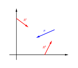
Figure 1. Drift $\mu$ and reflection vectors $R^{1}$ and $R^{2}$

Proposition 2.

The reflected Brownian motion $Z(t)$ associated with $(\Sigma,\mu,R)$ is well defined, and its stationary distribution $\Pi$ exists and is unique if and only if the data satisfy the following conditions:

$$r_{11}>0,\ \ r_{22}>0,\ \ r_{11}r_{22}-r_{12}r_{21}>0,$$ (1)

$$r_{22}\mu_{1}-r_{12}\mu_{2}<0,\ \ r_{11}\mu_{2}-r_{21}\mu_{1}<0.$$ (2)

The proof and some more detailed statements can be found in [24, 41, 20]. From now on we assume that conditions (1) and (2) are satisfied. The stationary distribution $\Pi$ is absolutely continuous with respect to Lebesgue measure as it is shown in [22] and [4]. We denote its density by $\pi(x_{1},x_{2})$.

1.3. Functional equation for the stationary distribution

Let $A$ be the generator of $(W_{t}+\mu t)_{t\geqslant 0}$. For each $f\in\mathcal{C}^{2}_{b}({\bf R}_{+}^{2})$ (the set of twice continuously differentiable functions $f$ on ${\bf R}_{+}^{2}$ such that $f$ and its first and second order derivatives are bounded) one has

$$Af(z)=\frac{1}{2}\sum_{i,j=1}^{2}\sigma_{i,j}\frac{\partial^{2}f}{\partial z_{i}\partial z_{j}}(z)+\sum_{i=1}^{2}\mu_{i}\frac{\partial f}{\partial z_{i}}(z).$$

Let us define for $i=1,2$,

$$D_{i}f(x)=\langle R^{i}|\nabla f\rangle$$

that may be interpreted as generators on the axes. We define now $\nu_{1}$ and $\nu_{2}$ two finite boundary measures with their support on the axes: for any Borel set $B\subset{\bf R}_{+}^{2}$,

$$\nu_{i}(B)=\mathbb{E}_{\Pi}[\int_{0}^{1}1_{\{Z(u)\in B\}}\mathrm{d}L^{i}(u)].$$

By definition of stationary distribution, for all $t\geqslant 0$, $\mathbb{E}_{\Pi}[f(Z(t))]=\int_{{\bf R}_{+}^{2}}f(z)\Pi(\mathrm{d}z)$. A similar formula holds true for $\nu_{i}$: $\mathbb{E}_{\Pi}[\int_{0}^{t}f(Z(u))\mathrm{d}L^{i}(u)]=t\int_{{\bf R}_{+}^{2}}f(x)\nu_{i}(\mathrm{d}x)$. Therefore $\nu_{1}$ and $\nu_{2}$ may be viewed as a kind of boundary invariant measures. The basic adjoint relationship takes the following form: for each $f\in\mathcal{C}^{2}_{b}({\bf R}_{+}^{2})$,

$$\int_{{\bf R}_{+}^{2}}Af(z)\Pi(\mathrm{d}z)+\sum_{i=1,2}\int_{{\bf R}_{+}^{2}}D_{i}f(z)\nu_{i}(\mathrm{d}z)=0.$$ (3)

The proof can be found in [22] in some particular cases and then has been extended to a general case, for example in [5]. We now define $\varphi(\theta)$ the two-dimensional Laplace transform of $\Pi$ also called its moment generating function. Let

$$\varphi(\theta)=\mathbb{E}_{\Pi}[\exp(\langle\theta|Z\rangle)]=\iint_{{\bf R}_{+}^{2}}\exp(\langle\theta|z\rangle)\Pi(\mathrm{d}z)$$

for all $\theta=(\theta_{1},\theta_{2})\in\mathbb{C}^{2}$ such that the integral converges. It does of course for any $\theta$ with ${\Re}\,\theta_{1}\leqslant 0,{\Re}\,\theta_{2}\leqslant 0$. We have set $\langle\theta|Z\rangle=\theta_{1}Z^{1}+\theta_{2}Z^{2}$. Likewise we define the moment generating functions for $\nu_{1}(\theta_{2})$ and $\nu_{2}(\theta_{1})$ on ${\bf C}$:

$$\varphi_{2}(\theta_{1})=\mathbb{E}_{\Pi}[\int_{0}^{1}e^{\theta_{1}Z_{t}^{1}}\mathrm{d}L^{2}(t)]=\int_{{\bf R}_{+}^{2}}e^{\theta_{1}z}\nu_{2}(\mathrm{d}z),\ \varphi_{1}(\theta_{2})=\mathbb{E}_{\Pi}[\int_{0}^{1}e^{\theta_{2}Z_{t}^{2}}\mathrm{d}L^{1}(t)]=\int_{{\bf R}_{+}^{2}}e^{\theta_{2}z}\nu_{1}(\mathrm{d}z).$$

Function $\varphi_{2}(\theta_{1})$ exists a priori for any $\theta_{1}$ with ${\Re}\,\theta_{1}\leqslant 0$. It is proved in [6] that it also does for $\theta_{1}$ with ${\Re}\,\theta_{1}\in[0,\epsilon_{1}]$, up to its first singularity $\epsilon_{1}>0$, the same is true for $\varphi_{1}(\theta_{2})$. The following key functional equation (proven in [6]) results from the basic adjoint relationship (3).

Theorem 3.

For any $\theta\in{\bf R}_{+}^{2}$ such $\varphi(\theta)<\infty$, $\varphi_{2}(\theta_{1})<\infty$ and $\varphi_{1}(\theta_{2})<\infty$ we have the following fundamental functional equation:

$$\gamma(\theta)\varphi(\theta)=\gamma_{1}(\theta)\varphi_{1}(\theta_{2})+\gamma_{2}(\theta)\varphi_{2}(\theta_{1}),$$ (4)

where

$$\begin{cases}\gamma(\theta)=-\frac{1}{2}\langle\theta|\Sigma\theta\rangle-\langle\theta|\mu\rangle=-\frac{1}{2}(\sigma_{11}\theta_{1}^{2}+\sigma_{22}\theta_{2}^{2}+2\sigma_{12}\theta_{1}\theta_{2})-(\mu_{1}\theta_{1}+\mu_{2}\theta_{2}),\\ \gamma_{1}(\theta)=\langle R^{1}|\theta\rangle=r_{11}\theta_{1}+r_{21}\theta_{2},\\ \gamma_{2}(\theta)=\langle R^{2}|\theta\rangle=r_{12}\theta_{1}+r_{22}\theta_{2}.\end{cases}$$ (5)

This equation holds true a priori for any $\theta=(\theta_{1},\theta_{2})$ with ${\Re}\,\theta_{1}\leqslant 0,{\Re}\,\theta_{2}\leqslant 0$. It plays a crucial role in the analysis of the stationary distribution.

1.4. Results

Our aim is to obtain the asymptotic expansion of the stationary distribution density $\pi(x)=\pi(x_{1},x_{2})$ as $x_{1},x_{2}\to\infty$ and $x_{2}/x_{1}\to{\rm tan}\,(\alpha_{0})$ for any given angle $\alpha_{0}\in[0,\pi/2]$.

Notation. We write the asymptotic expansion $f(x)\sim\sum_{k=0}^{n}g_{k}(x)$ as $x\to x_{0}$ if $g_{k}(x)=o(g_{k-1}(x))$ as $x\to x_{0}$ for all $k=1,\ldots,n$ and $f(x)-\sum_{k=0}^{n}g_{k}(x)=o(g_{n}(x))$ as $x\to x_{0}$.

It will be more convenient to expand $\pi(r\cos\alpha,r\sin\alpha)$ as $r\to\infty$ and $\alpha\to\alpha_{0}$. We give our final results in Section 5, Theorems 22–25: we find the expansion of $\pi(r\cos\alpha,r\sin\alpha)$ as $r\to\infty$ and prove it uniform for $\alpha$ fixed in a small neighborhood $\mathcal{O}(\alpha_{0})\subset]0,\pi/2[$ of $\alpha_{0}\in]0,\pi/2[$.

In this section, Theorem 4 below announces the main term of the expansion depending on parameters $(\mu,\Sigma,R)$ and a given direction $\alpha_{0}$. Next, in Section 1.5 we sketch our analytic approach following the main lines of this paper in order to get the full asymptotic expansion of $\pi$. We present at the same time the organization of the article.

Now we need to introduce some notations. The quadratic form $\gamma(\theta)$ is defined in (4) via the covariance matrix $\Sigma$ and the drift $\mu$ of the process in the interior of ${\bf R}_{+}^{2}$. Let us restrict ourselves on $\theta\in{\bf R}^{2}$. The equation $\gamma(\theta)=0$ determines an ellipse $\mathcal{E}$ on ${\bf R}^{2}$ passing through the origin, its tangent in it is orthogonal to vector $\mu$, see Figure 2. Stability conditions (1) and (2) imply the negativity of at least one of coordinates of $\mu$, see [6, Lemma 2.1]. In this article, in order to shorten the number of pictures and cases of parameters to consider, we restrict ourselves to the case

$$\mu_{1}<0\text{ and }\mu_{2}<0,$$ (6)

although our methods can be applied without any difficulty to other cases, we briefly sketch some different details at the end of Section 2.4.

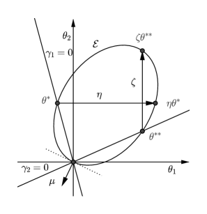
Figure 2. Ellipse $\mathcal{E}$, straight lines $\gamma_{1}(\theta)=0$, $\gamma_{2}(\theta)=0$, points $\theta^{*},\theta^{**},\eta\theta^{*},\zeta\theta^{**}$

Let us call $s_{1}^{+}=(\theta_{1}(s_{1}^{+}),\theta_{2}(s_{1}^{+}))\in{\cal E}$ the point of the ellipse with the maximal first coordinate: $\theta_{1}(s_{1}^{+})=\sup\{\theta_{1}:\gamma(\theta_{1},\theta_{2})=0\}$. Let us call $s_{2}^{+}$ the point of the ellipse with the maximal second coordinate. Let ${\cal A}$ be the arc of the ellipse with endpoints $s_{1}^{+}$, $s_{2}^{+}$ not passing through the origin, see Figure 3. For a given angle $\alpha\in[0,\pi/2]$ let us define the point $\theta(\alpha)$ on the arc ${\cal A}$ as

$$\theta(\alpha)={\rm argmax}_{\theta\in{\cal A}}\langle\theta\mid e_{\alpha}\rangle\ \ \hbox{where }e_{\alpha}=(\cos\alpha,\sin\alpha).$$ (7)

Note that $\theta(0)=s_{1}^{+}$, $\theta(\pi/2)=s_{2}^{+}$, and $\theta(\alpha)$ is an isomorphism between $[0,\pi/2]$ and ${\cal A}$. Coordinates of $\theta(\alpha)$ are given explicitly in (50). One can also construct $\theta(\alpha)$ geometrically: first draw a ray $r(\alpha)$ on ${\bf R}_{+}^{2}$ that forms the angle $\alpha$ with $\theta_{1}$-axis, and then the straight line $l(\alpha)$ orthogonal to this ray and tangent to the ellipse. Then $\theta(\alpha)$ is the point where $l(\alpha)$ is tangent to the ellipse, see Figure 3.

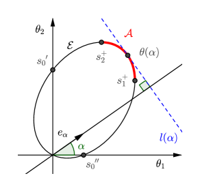
Figure 3. Arc $\cal{A}$ and point $\theta(\alpha)$ on $\cal{E}$

Secondly, consider the straight lines $\gamma_{1}(\theta)=0$, $\gamma_{2}(\theta)=0$ defined in (4) via the reflection matrix $R$. They cross the ellipse ${\cal E}$ in the origin. Furthermore, due to stability conditions (1) and (2) the line $\gamma_{1}(\theta)=0$ [resp. $\gamma_{2}(\theta)=0$] intersects the ellipse at the second point $\theta^{*}=(\theta_{1}^{*},\theta_{2}^{*})$ (resp. $\theta^{**}=(\theta_{1}^{**},\theta_{2}^{**})$) where $\theta_{2}^{*}>0$ (resp. $\theta_{1}^{**}>0$). Stability conditions also imply that the ray $\gamma_{1}(\theta)=0$ is always "above" the ray $\gamma_{2}(\theta)=0$, see [6, Lemma 2.2]. To present our results, we need to define the images of these points via the so-called Galois automorphisms $\zeta$ and $\eta$ of ${\cal E}$. Namely, for point $\theta^{*}=(\theta_{1}^{*},\theta_{2}^{*})\in{\cal E}$ there exists a unique point $\eta\theta^{*}=(\eta\theta_{1}^{*},\theta_{2}^{*})\in{\cal E}$ that has the same second coordinate. Clearly, $\theta_{1}^{*}$ and $\eta\theta_{1}^{*}$ are two roots of the second degree equation $\gamma(\cdot,\theta_{2}^{*})=0.$ In the same way for point $\theta^{**}=(\theta_{1}^{**},\theta_{2}^{**})\in{\cal E}$ there exists a unique point $\zeta\theta^{**}=(\theta_{1}^{**},\zeta\theta_{2}^{**})\in{\cal E}$ with the same first coordinate. Points $\theta_{2}^{**}$ and $\zeta\theta_{2}^{**}$ are two roots of the second degree equation $\gamma(\theta_{1}^{**},\cdot)=0.$ Points $\theta^{*}$, $\theta^{**}$, $\eta\theta^{*}$ and $\zeta\theta^{**}$ are pictured on Figure 2. Their coordinates are made explicit in (33) and (34).

Finally let $s^{\prime}_{0}=(0,-2\frac{\mu_{22}}{\sigma_{22}})$ be the point of intersection of the ellipse $\mathcal{E}$ with $\theta_{2}$-axis and let $s^{\prime\prime}_{0}=(-2\frac{\mu_{11}}{\sigma_{11}},0)$ be the point of intersection of the ellipse with $\theta_{1}$-axis, see Figure 3. The following theorem provides the main asymptotic term of $\pi(r\cos\alpha,r\sin\alpha)$.

Theorem 4.

Let $\alpha_{0}\in]0,\pi/2[$. Let $\theta(\alpha)$ be defined in (7). Let $\color[rgb]{1,0,0}\{\theta(\alpha_{0}),s^{\prime}_{0}\}$ (resp. $\color[rgb]{0,0,1}\{s^{\prime\prime}_{0},\theta(\alpha_{0})\}$) be the arc of the ellipse ${\cal E}$ with end points $s^{\prime}_{0}$ and $\theta(\alpha_{0})$ (resp. $s^{\prime\prime}_{0}$ and $\theta(\alpha_{0})$) not passing through the origin. We have the following results.

• If $\zeta\theta^{**}\notin\{\theta(\alpha_{0}),s^{\prime}_{0}\}$ and $\eta\theta^{*}\notin\{s^{\prime\prime}_{0},\theta(\alpha_{0})\}$, then there exists a constant $c(\alpha_{0})$ such that

  $$\pi(r\cos\alpha,r\sin\alpha)\sim\frac{c(\alpha_{0})}{\sqrt{r}}\exp\Big{(}-r\langle e_{\alpha}\mid\theta(\alpha)\rangle\Big{)}\ \ \ r\to\infty,\alpha\to\alpha_{0}.$$ (8)

  The function $c(\alpha)$ varies continuously on $[0,\pi/2]$, $\lim_{\alpha\to 0}c(\alpha)=\lim_{\alpha\to\pi/2}c(\alpha)=0$.

• If $\zeta\theta^{**}\in\}\theta(\alpha_{0}),s^{\prime}_{0}\}$ and $\eta\theta^{*}\notin\{s^{\prime\prime}_{0},\theta(\alpha_{0})\{$, then with some constant $c_{1}>0$

  $$\pi(r\cos\alpha,r\sin\alpha)\sim c_{1}\exp\Big{(}-r\langle e_{\alpha}\mid\zeta\theta^{**}\rangle\Big{)}\ \ r\to\infty,\alpha\to\alpha_{0}.$$ (9)

• If $\zeta\theta^{**}\notin\}\theta(\alpha_{0}),s^{\prime}_{0}\}$ and $\eta\theta^{*}\in\{s^{\prime\prime}_{0},\theta(\alpha_{0})\{$, then with some constant $c_{2}>0$

  $$\pi(r\cos\alpha,r\sin\alpha)\sim c_{2}\exp\Big{(}-r\langle e_{\alpha}\mid\eta\theta^{*}\rangle\Big{)}\ \ r\to\infty,\alpha\to\alpha_{0}.$$ (10)

• Let $\zeta\theta^{**}\in\}\theta(\alpha_{0}),s^{\prime}_{0}\}$ and $\eta\theta^{*}\in\{s^{\prime\prime}_{0},\theta(\alpha_{0})\{$. If $\langle\zeta\theta^{**}\mid e_{\alpha_{0}}\rangle<\langle\eta\theta^{*}\mid e_{\alpha_{0}}\rangle$, then the asymptotics (9) is valid with some constant $c_{1}>0$. If $\langle\zeta\theta^{**}\mid e_{\alpha_{0}}\rangle>\langle\eta\theta^{*}\mid e_{\alpha_{0}}\rangle$, then the asymptotics (10) is valid with some constant $c_{2}>0$. If $\langle\zeta\theta^{**}\mid e_{\alpha_{0}}\rangle=\langle\eta\theta^{*}\mid e_{\alpha_{0}}\rangle$, then then with some constants $c_{1}>0$ and $c_{2}>0$

  $$\pi(r\cos\alpha,r\sin\alpha)\sim c_{1}\exp\Big{(}-r\langle e_{\alpha}\mid\zeta\theta^{**}\rangle\Big{)}+c_{2}\exp\Big{(}-r\langle e_{\alpha}\mid\eta\theta^{*}\rangle\Big{)}\ \ \ r\to\infty,\alpha\to\alpha_{0}.$$ (11)

See Figure 4 for the different cases. (The arcs $\}a,b\}$ or $\{a,b\{$ of $\mathcal{E}$ are those not passing through the origin where the left or the right end respectively is excluded).

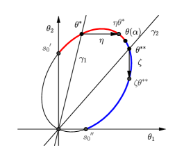
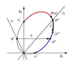
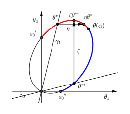
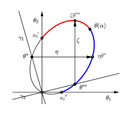
Figure 4. Cases (1),(2),(3),(4)

Let us note that the exponents in Theorem 4 are the same as in the large deviation rate function found in [7, Thm 3.2]. The same phenomenon is observed for discrete random walks, cf. [36] and [25].

1.5. Sketch of the analytic approach. Organization of the paper

The starting point of our approach is the main functional equation (4) valid for any $\theta=(\theta_{1},\theta_{2})\in{\bf C}^{2}$ with ${\Re}\,\theta_{1}\leqslant 0$, ${\Re}\,\theta_{2}\leqslant 0$. The function $\gamma(\theta_{1},\theta_{2})$ in the left-hand side is a polynomial of the second order of $\theta_{1}$ and $\theta_{2}$. The algebraic function $\Theta_{1}(\theta_{2})$ defined by $\gamma(\Theta_{1}(\theta_{2}),\theta_{2})\equiv 0$ is $2$-valued and its Riemann surface ${\bf S}_{\theta_{2}}$ is of genus $0$. The same is true about the $2$-valued algebraic function $\Theta_{2}(\theta_{1})$ defined by $\gamma(\theta_{1},\Theta_{2}(\theta_{1}))=0$ and its Riemann surface ${\bf S}_{\theta_{1}}$. The surfaces ${\bf S}_{\theta_{1}}$ and ${\bf S}_{\theta_{2}}$ being equivalent, we will consider just one surface ${\bf S}$ defined by the equation $\gamma(\theta_{1},\theta_{2})=0$ with two different coverings. Each point $s\in\mathbf{S}$ has two “coordinates” $(\theta_{1}(s),\theta_{2}(s))$, both of them are complex or infinite and satisfy $\gamma(\theta_{1}(s),\theta_{2}(s))=0$. For any point $s=(\theta_{1},\theta_{2})\in\mathbf{S}$, there exits a unique point $s^{\prime}=(\theta_{1},\theta^{\prime}_{2})\in\mathbf{S}$ with the same first coordinate and there exists a unique point $s^{\prime\prime}=(\theta^{\prime\prime}_{1},\theta_{2})\in\mathbf{S}$ with the same second coordinate. We say that $s^{\prime}=\zeta s$, i.e. $s^{\prime}$ and $s$ are related by Galois automorphism $\zeta$ of ${\bf S}$ that leaves untouched the first coordinate, and that $s^{\prime\prime}=\eta s$, i.e. $s^{\prime\prime}$ and $s$ are related by Galois automorphism $\eta$ of ${\bf S}$ that leaves untouched the second coordinate. Clearly $\zeta^{2}=Id$, $\eta^{2}=Id$ and the branch points of $\Theta_{1}(\theta_{2})$ and of $\Theta_{2}(\theta_{1})$ are fixed points of $\zeta$ and $\eta$ respectively. The ellipse $\mathcal{E}$ is the set of points of ${\bf S}$ where both “coordinates” are real. The construction of ${\bf S}$ and definition of Galois automorphisms are carried out in Section 2.

Next, unknown functions $\varphi_{1}(\theta_{2})$ and $\varphi_{2}(\theta_{1})$ are lifted in the domains of $\mathbf{S}$ where $\{s\in\mathbf{S}:{\Re}\,\theta_{2}(s)\leqslant 0\}$ and $\{s\in\mathbf{S}:{\Re}\,\theta_{1}(s)\leqslant 0\}$ respectively. The intersection of these domains on ${\bf S}$ is non-empty, both $\varphi_{2}$ and $\varphi_{1}$ are well defined in it. Since for any $s=(\theta_{1}(s),\theta_{2}(s))\in\mathbf{S}$ we have $\gamma(\theta_{1}(s),\theta_{2}(s))=0$, the main functional equation (4) implies:

$$\gamma_{1}(\theta_{1}(s),\theta_{2}(s))\varphi_{1}(\theta_{2}(s))+\gamma_{2}(\theta_{1}(s),\theta_{2}(s))\varphi_{2}(\theta_{1}(s))=0\ \ \forall s\in\mathbf{S},{\Re}\,\theta_{1}(s)\leqslant 0,{\Re}\,\theta_{2}(s)\leqslant 0.$$

Using this relation, Galois automorphisms and the facts that $\varphi_{1}$ and $\varphi_{2}$ depend just on one ”coordinate” ($\varphi_{1}$ depends on $\theta_{2}$ and $\varphi_{2}$ on $\theta_{1}$ only), we continue $\varphi_{1}$ and $\varphi_{2}$ explicitly as meromorphic on the whole of $\mathbf{S}$. This meromorphic continuation procedure is the crucial step of our approach, it is the subject of Section 3.1. It allows to recover $\varphi_{1}$ and $\varphi_{2}$ on the complex plane as multivalued functions and determines all poles of all its branches. Namely, it shows that poles of $\varphi_{1}$ and $\varphi_{2}$ may be only at images of zeros of $\gamma_{1}$ and $\gamma_{2}$ by automorphisms $\eta$ and $\zeta$ applied several times. We are in particular interested in the poles of their first (main) branch, and more precisely in the most ”important” pole (from the asymptotic point of view, to be explained below), that turns out to be at one of points $\zeta\theta^{**}$ or $\eta\theta^{*}$ defined above. The detailed analysis of the "main" poles of $\varphi_{1}$ and $\varphi_{2}$ is furnished in Section 3.2.

Let us now turn to the asymptotic expansion of the density $\pi(x_{1},x_{2})$. Its Laplace transform comes from the right-hand side of the main equation (4) divided by the kernel $\gamma(\theta_{1},\theta_{2})$. By inversion formula the density $\pi(x_{1},x_{2})$ is then represented as a double integral on $\{\theta:{\Re}\,\theta_{1}={\Re}\,\theta_{2}=0\}$. In Section 4.1, using the residues of the function $\frac{1}{\gamma(\theta_{1},\cdot)}$ or $\frac{1}{\gamma(\cdot,\theta_{2})}$ we transform this double integral into a sum of two single integrals along two cycles on $\mathbf{S}$, those where ${\Re}\,\theta_{1}(s)=0$ or ${\Re}\,\theta_{2}(s)=0$. Putting $(x_{1},x_{2})=re_{\alpha}$ we get the representation of the density as a sum of two single integrals along some contours on ${\bf S}$:

$$\pi(re_{\alpha})=\frac{1}{2\pi\sqrt{\det\Sigma}}\big{(}\int_{\mathcal{I}_{\theta_{1}}^{+}}\frac{\varphi_{2}(s)\gamma_{2}(\theta(s))}{s}e^{-r\langle\theta(s)\mid e_{\alpha}\rangle}{\mathrm{d}s}+\int_{\mathcal{I}_{\theta_{2}}^{+}}\frac{\varphi_{1}(s)\gamma_{1}(\theta(s))}{s}e^{-r\langle\theta(s)\mid e_{\alpha}\rangle}\mathrm{d}s\big{)}.$$ (12)

We would like to compute their asymptotic expansion as $r\to\infty$ and prove it to be uniform for $\alpha$ fixed in a small neighborhood $\mathcal{O}(\alpha_{0})$, $\alpha_{0}\in]0,\pi/2[$.

These two integrals are typical to apply the saddle-point method, see [15, 37]. The point $\theta(\alpha)\in\mathcal{E}$ defined above is the saddle-point for both of them, this is the subject of Section 4.2. The integration contours on ${\bf S}$ are then shifted to new ones $\Gamma_{\theta_{1},\alpha}$ and $\Gamma_{\theta_{2},\alpha}$ which are constructed in such a way that they pass through the saddle-point $\theta(\alpha)$, follow the steepest-descent curve in its neighborhood $\mathcal{O}(\theta(\alpha))$ and are “higher” than the saddle-point w.r.t. the level curves of the function $\langle\theta(s)\mid e_{\alpha}\rangle$ outside $\mathcal{O}(\theta(\alpha))$, see Section 4.3. Applying Cauchy Theorem, the density is finally represented as a sum of integrals along these new contours and the sum of residues at poles of the integrands we encounter deforming the initial ones:

$$\pi(re_{\alpha})=\sum_{p\in{\cal P^{\prime}}_{\alpha}}{\rm res}_{p}\varphi_{2}(\theta_{1}(s))\frac{\gamma_{2}(p)}{\sqrt{d(\theta_{1}(p))}}e^{-r\langle\theta(p)\mid e_{\alpha}\rangle}+\sum_{p\in{\cal P^{\prime\prime}}_{\alpha}}{\rm res}_{p}\varphi_{1}(\theta_{2}(s))\frac{\gamma_{1}(p)}{\sqrt{\tilde{d}(\theta_{2}(p))}}e^{-r\langle\theta(p)\mid e_{\alpha}\rangle}\\ \frac{1}{2\pi\sqrt{\det\Sigma}}\left(\int_{\Gamma_{\theta_{1},\alpha}}\frac{\varphi_{2}(s)\gamma_{2}(\theta(s))}{s}e^{-r\langle\theta(s)\mid e_{\alpha}\rangle}{\mathrm{d}s}+\int_{\Gamma_{\theta_{2},\alpha}}\frac{\varphi_{1}(s)\gamma_{1}(\theta(s))}{s}e^{-r\langle\theta(s)\mid e_{\alpha}\rangle}\mathrm{d}s\right).$$ (13)

Here ${\cal P}^{\prime}_{\alpha}$ (resp. ${\cal P^{\prime\prime}}_{\alpha}$) is the set of poles of the first order of $\varphi_{1}$ (resp. $\varphi_{2}$) that are found when shifting the initial contour $\mathcal{I}_{\theta_{1}}^{+}$ to the new one $\Gamma_{\theta_{1},\alpha}$ (resp. $\mathcal{I}_{\theta_{2}}^{+}$ to $\Gamma_{\theta_{2},\alpha}$), all of them are on the arc $\{s^{\prime}_{0},\theta(\alpha)\}$ (resp. $\{\theta(\alpha),s^{\prime\prime}_{0}\}$) of ellipse $\mathcal{E}$.

The asymptotic expansion of integrals along $\Gamma_{\theta_{1},\alpha}$ and $\Gamma_{\theta_{2},\alpha}$ is made explicit by the standard saddle-point method in Section 4.4. The set of poles ${\cal P}^{\prime}_{\alpha}\cup{\cal P^{\prime\prime}}_{\alpha}$ is analyzed in Section 4.5 . In Case (1) of Theorem 4 this set is empty, thus the asymptotic expansion of the density is determined by the saddle-point, its first term is given in Theorem 4. In Cases (2), (3) and (4) this set is not empty. The residues at poles over ${\cal P}^{\prime}_{\alpha}\cup{\cal P^{\prime\prime}}_{\alpha}$ in (13) bring all more important contribution to the asymptotic expansion of $\pi(re_{\alpha})$ than the integrals along $\Gamma_{\theta_{1},\alpha}$ and $\Gamma_{\theta_{2},\alpha}$. Taking into account the monotonicity of function $\langle\theta\mid e_{\alpha}\rangle$ on the arcs $\{s^{\prime\prime}_{0},\theta(\alpha)\}$ and on $\{\theta(\alpha),s^{\prime}_{0}\}$, they can be ranked in order of their importance: clearly, the term associated with a pole $p^{\prime}$ is more important than the one with $p^{\prime\prime}$ if $\langle p^{\prime}\mid e_{\alpha}\rangle<\langle p^{\prime\prime}\mid e_{\alpha}\rangle$. In Case (2) (resp. (3)) the most important pole is $\zeta\theta^{**}$ (resp. $\eta\theta^{*}$), as announced in Theorem 4. In Case (4) the most important of them is among $\zeta\theta^{**}$ and $\eta\theta^{*}$, as stated in Theorem 4 as well. The expansion of integrals in (13) along $\Gamma_{\theta_{1},\alpha}$ and $\Gamma_{\theta_{2},\alpha}$ via the saddle-point method provides all smaller asymptotic terms than those coming from the poles. Section 5 is devoted to the results: they are stated from two points of view in Sections 5.1 and 5.2 respectively. First, given an angle $\alpha_{0}$, we find the uniform asymptotic expansion of the density $\pi(r\cos(\alpha),r\sin(\alpha))$ as $r\to\infty$ and $\alpha\in\mathcal{O}(\alpha_{0})$ depending on parameters $(\Sigma,\mu,R)$: Theorems 22 –25 of Section 5.1 state it in all cases of parameters (1)–(4). Second, in Section 5.2, given a set parameters $(\Sigma,\mu,R)$, we compute the asymptotics of the density for all angles $\alpha_{0}\in]0,\pi/2[$, see Theorems 26-28.

Remark. The constants mentioned in Theorem 4 and all those in asymptotic expansions of Theorems 22–28 are specified in terms of functions $\varphi_{1}$ and $\varphi_{2}$. In the present paper we leave unknown these functions in their initial domains of definition although we carry out explicitly their meromorphic continuation procedure and find all their poles. In [18] the first author and K. Raschel make explicit these functions solving some boundary value problems. This determines the constants in asymptotic expansions in Theorems 4, 22–28 .

Future works. The case of parameters such that $\zeta\theta^{**}=\theta(\alpha)$ and $\eta\theta^{*}\not\in\{s^{\prime}_{0},\theta(\alpha)\{$ or the case such that $\eta\theta^{*}=\theta(\alpha)$ and $\zeta\theta^{**}\not\in\{s^{\prime\prime}_{0},\theta(\alpha)\{$ are not treated in Theorem 4. Theorem 25 gives a partial result but not at all as satisfactory as in all other cases. In fact, in these cases the saddle-point $\theta(\alpha)$ coincides with the “main” pole of $\varphi_{1}$ or $\varphi_{2}$. The analysis is then reduced to a technical problem of computing the asymptotics of an integral whenever the saddle-point coincides with a pole of the integrand or approaches to it. We leave it for the future work.

In the cases $\alpha=0$ and $\alpha=\pi/2$, the tail asymptotics of the boundary measures $\nu_{1}$ and $\nu_{2}$ has been found in [7] and the constants have been specified in [18]. It would be also possible to find the asymptotics of $\pi(r\cos\alpha,r\sin\alpha)$ where $r\to\infty$ and $\alpha\to 0$ or $\alpha\to\pi/2$. This problem is reduced to obtaining the asymptotics of an integral when the saddle-point $\theta(0)$ or $\theta(\pi/2)$ coincides with a branch point of the integrand $\varphi_{1}$ or $\varphi_{2}$. It can be solved by the same methods as in [26] for discrete random walks.

2. Riemann surface $\mathbf{S}$

2.1. Kernel $\gamma(\theta_{1},\theta_{2})$

The kernel of the main functional equation

$$\gamma(\theta_{1},\theta_{2})=\frac{1}{2}(\sigma_{11}\theta_{1}^{2}+\sigma_{22}\theta_{2}^{2}+2\sigma_{12}\theta_{1}\theta_{2})+\mu_{1}\theta_{1}+\mu_{2}\theta_{2}$$

can be written as

$$\gamma(\theta_{1},\theta_{2})=\tilde{a}(\theta_{2})\theta_{1}^{2}+\tilde{b}(\theta_{2})\theta_{1}+\tilde{c}(\theta_{2})=a(\theta_{1})\theta_{2}^{2}+b(\theta_{1})\theta_{2}+c(\theta_{1})$$

where

$\tilde{a}(\theta_{2})=\frac{1}{2}\sigma_{11}$,	$\tilde{b}(\theta_{2})=\sigma_{12}\theta_{2}+\mu_{1}$,	$\tilde{c}(\theta_{2})=\frac{1}{2}\sigma_{22}\theta_{2}^{2}+\mu_{2}\theta_{2}$,
$a(\theta_{1})=\frac{1}{2}\sigma_{22}$,	$b(\theta_{1})=\sigma_{12}\theta_{1}+\mu_{2}$,	$c(\theta_{1})=\frac{1}{2}\sigma_{11}\theta_{1}^{2}+\mu_{1}\theta_{1}$.

The equation $\gamma(\theta_{1},\theta_{2})\equiv 0$ defines a two-valued algebraic function $\Theta_{1}(\theta_{2})$ such that $\gamma(\Theta_{1}(\theta_{2}),\theta_{2})\equiv 0$ and a two-valued algebraic function $\Theta_{2}(\theta_{1})$ such that $\gamma(\theta_{1},\Theta_{2}(\theta_{1})\equiv 0$. These functions have two branches:

$\Theta_{1}^{+}(\theta_{2})=\frac{-\tilde{b}(\theta_{2})+\sqrt{\tilde{d}(\theta_{2})}}{2\tilde{a}(\theta_{2})}$,

$\Theta_{1}^{-}(\theta_{2})=\frac{-\tilde{b}(\theta_{2})-\sqrt{\tilde{d}(\theta_{2})}}{2\tilde{a}(\theta_{2})}$,

and

$\Theta_{2}^{+}(\theta_{1})=\frac{-b(\theta_{1})+\sqrt{d(\theta_{1})}}{2a(\theta_{1})}$,

$\Theta_{2}^{-}(\theta_{1})=\frac{-b(\theta_{1})-\sqrt{d(\theta_{1})}}{2a(\theta_{1})}$.

where

$\tilde{d}(\theta_{2})=\theta_{2}^{2}(\sigma_{12}^{2}-\sigma_{11}\sigma_{22})+2\theta_{2}(\mu_{1}\sigma_{12}-\mu_{2}\sigma_{11})+\mu_{1}^{2}$,

$d(\theta_{1})=\theta_{1}^{2}(\sigma_{12}^{2}-\sigma_{11}\sigma_{22})+2\theta_{1}(\mu_{2}\sigma_{12}-\mu_{1}\sigma_{22})+\mu_{2}^{2}$.

The discriminant ${d}(\theta_{1})$ (resp. $\tilde{d}(\theta_{2})$) has two zeros $\theta_{1}^{+}$, $\theta_{1}^{-}$ (resp. $\theta_{2}^{+}$ and $\theta_{2}^{-}$) that are both real and of opposite signs:

$\theta_{1}^{-}=\frac{(\mu_{2}\sigma_{12}-\mu_{1}\sigma_{22})-\sqrt{D_{1}}}{\det{\Sigma}}<0$,

$\theta_{1}^{+}=\frac{(\mu_{2}\sigma_{12}-\mu_{1}\sigma_{22})+\sqrt{D_{1}}}{\det{\Sigma}}>0$,

$\theta_{2}^{-}=\frac{(\mu_{1}\sigma_{12}-\mu_{2}\sigma_{11})-\sqrt{D_{2}}}{\det{\Sigma}}<0$,

$\theta_{2}^{+}=\frac{(\mu_{1}\sigma_{12}-\mu_{2}\sigma_{11})+\sqrt{D_{2}}}{\det{\Sigma}}>0$,

with notations $D_{1}=(\mu_{2}\sigma_{12}-\mu_{1}\sigma_{22})^{2}+\mu_{2}^{2}\det{\Sigma}$ and $D_{2}=(\mu_{1}\sigma_{12}-\mu_{2}\sigma_{11})^{2}+\mu_{1}^{2}\det{\Sigma}$. Then $\Theta_{2}(\theta_{1})$ (resp. $\Theta_{1}(\theta_{2})$) has two branch points: $\theta_{1}^{-}$ and $\theta_{1}^{+}$ (resp $\theta_{2}^{-}$ and $\theta_{2}^{+}$). We can compute:

$$\Theta_{2}^{\pm}(\theta_{1}^{-})=\frac{\mu_{1}\sigma_{12}-\mu_{2}\sigma_{11}+\frac{\sigma_{12}}{\sigma_{22}}\sqrt{D_{1}}}{\det\Sigma},\ \ \Theta_{2}^{\pm}(\theta_{1}^{+})=\frac{\mu_{1}\sigma_{12}-\mu_{2}\sigma_{11}-\frac{\sigma_{12}}{\sigma_{22}}\sqrt{D_{1}}}{\det\Sigma},$$

$$\Theta_{1}^{\pm}(\theta_{2}^{-})=\frac{\mu_{2}\sigma_{12}-\mu_{1}\sigma_{22}+\frac{\sigma_{12}}{\sigma_{11}}\sqrt{D_{2}}}{\det\Sigma},\ \ \Theta_{1}^{\pm}(\theta_{2}^{+})=\frac{\mu_{2}\sigma_{12}-\mu_{1}\sigma_{22}-\frac{\sigma_{12}}{\sigma_{11}}\sqrt{D_{2}}}{\det\Sigma}.$$

Furthermore, $d(\theta_{1})$ (resp. $\tilde{d}(\theta_{2})$) being positive on $]\theta_{1}^{-},\theta_{1}^{+}[$ (resp. $]\theta_{2}^{-},\theta_{2}^{+}[$) and negative on ${\bf R}\setminus[\theta_{1}^{-},\theta_{1}^{+}]$ (resp. ${\bf R}\setminus[\theta_{2}^{-},\theta_{2}^{+}]$) , both branches $\Theta_{2}^{\pm}(\theta_{1})$ (resp. $\Theta_{1}^{\pm}(\theta_{2})$) take real values on $[\theta_{1}^{-},\theta_{1}^{+}]$ (resp. $[\theta_{2}^{-},\theta_{2}^{+}]$) and complex values on ${\bf R}\setminus[\theta_{1}^{-},\theta_{1}^{+}]$ (resp. ${\bf R}\setminus[\theta_{2}^{-},\theta_{2}^{+}]$).

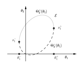
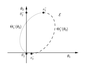
Figure 5. Functions $\Theta_{2}^{\pm}(\theta_{1})$ and $\Theta_{1}^{\pm}(\theta_{2})$ on $[\theta_{1}^{-},\theta_{1}^{+}]$ and $[\theta_{2}^{-},\theta_{2}^{+}]$

2.2. Construction of the Riemann surface ${\bf S}$

We now construct the Riemann surface $\mathbf{S}$ of the algebraic function $\Theta_{2}(\theta_{1})$. For this purpose we take two Riemann spheres $\mathbb{C}_{\theta_{1}}^{1}\cup\{\infty\}$ and $\mathbb{C}_{\theta_{1}}^{2}\cup\{\infty^{\prime}\}$, say $\mathbf{S}_{\theta_{1}}^{1}$ and $\mathbf{S}_{\theta_{1}}^{2}$, cut along $([-\infty^{(\prime)},\theta_{1}^{-}]\cup[\theta_{1}^{+},\infty^{(\prime)}])$, and we glue them together along the borders of these cuts, joining the lower border of the cut on $\mathbf{S}_{\theta_{1}}^{1}$ to the upper border of the same cut on $\mathbf{S}_{\theta_{1}}^{2}$ and vice versa. This procedure can be viewed as gluing together two half-spheres, see Figure 6. The resulting surface $\mathbf{S}$ is homeomorphic to a sphere (i.e., a compact Riemann surface of genus 0) and is projected on the Riemann sphere $\mathbb{C}\cup\{\infty\}$ by a canonical covering map $h_{\theta_{1}}:\mathbf{S}\to\mathbb{C}\cup\{\infty\}$. In a standard way, we can lift the function $\Theta_{2}(\theta_{1})$ to $\mathbf{S}$, by setting $\Theta_{2}(s)=\Theta_{2}^{+}(h_{\theta_{1}}(s))$ if $s\in\mathbf{S}_{\theta_{1}}^{1}\subset\mathbf{S}$ and $\Theta_{2}(s)=\Theta_{2}^{-}(h_{\theta_{1}}(s))$ if $s\in\mathbf{S}_{\theta_{1}}^{2}\subset\mathbf{S}$.

In a similar way one constructs the Riemann surface of the function $\Theta_{1}(\theta_{2})$, by gluing together two copies $\mathbf{S}_{\theta_{2}}^{1}$ and $\mathbf{S}_{\theta_{2}}^{2}$ of the Riemann sphere $\mathbf{S}$ cut along $([-\infty^{(\prime)},\theta_{2}^{-}]\cup[\theta_{2}^{+},\infty^{(\prime)}])$. We obtain again a surface homeomorphic to a sphere where we lift function $\Theta_{1}(\theta_{2})$.

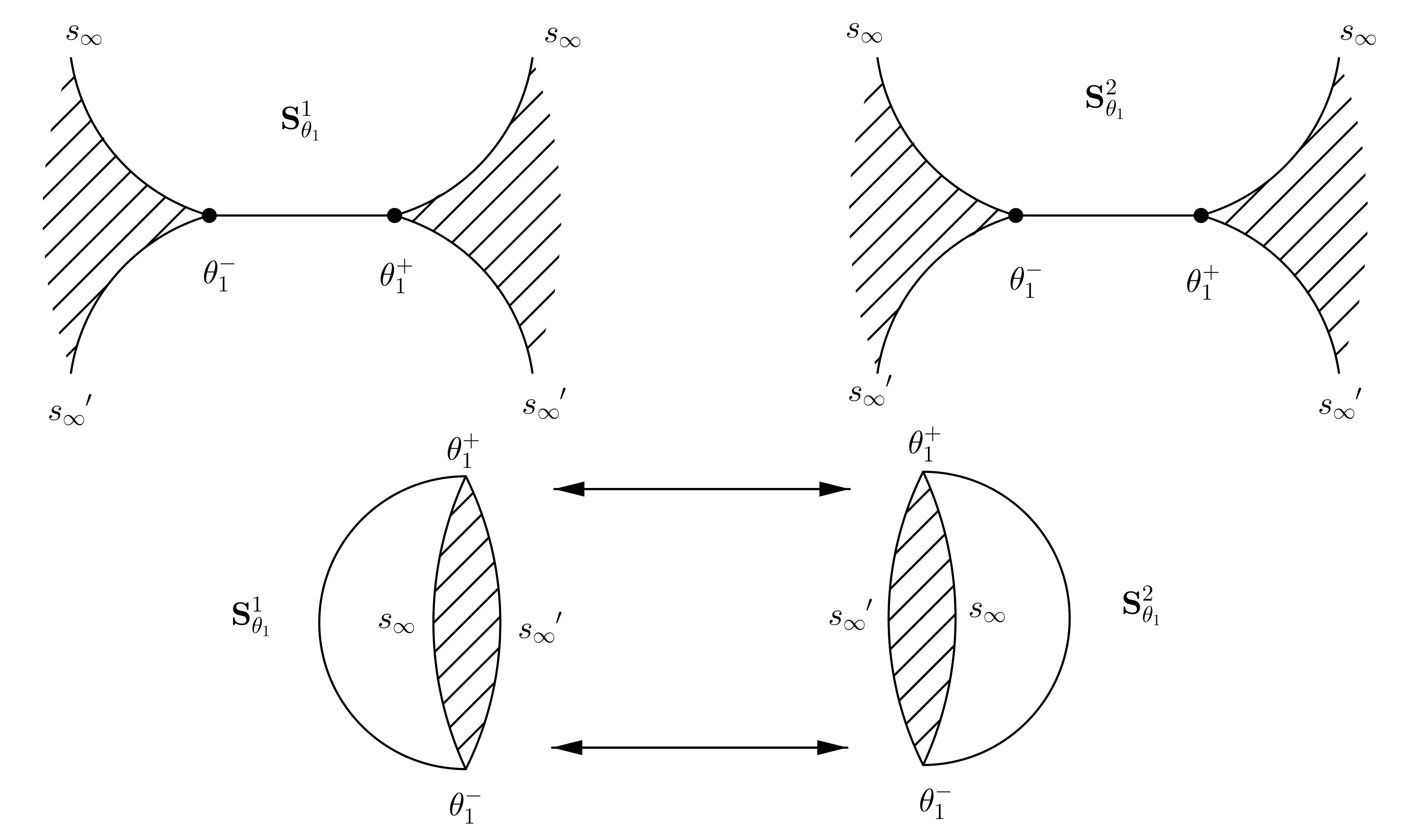
Figure 6. Construction of the Riemann surface $\mathbf{S}$

Since the Riemann surfaces of $\Theta_{1}(\theta_{2})$ and $\Theta_{2}(\theta_{1})$ are equivalent, we can and will work on a single Riemann surface $\mathbf{S}$, with two different covering maps $h_{\theta_{1}},h_{\theta_{2}}:\mathbf{S}\to\mathbb{C}\cup\{\infty\}$. Then, for $s\in\mathbf{S}$, we set $\theta_{1}(s)=h_{\theta_{1}}(s)$ and $\theta_{2}(s)=h_{\theta_{2}}(s)$. We will often represent a point $s\in\mathbf{S}$ by the pair of its coordinates $(\theta_{1}(s),\theta_{2}(s))$. These coordinates are of course not independent, because the equation $\gamma(\theta_{1}(s),\theta_{2}(s))=0$ is valid for any $s\in\mathbf{S}$. One can see ${\bf S}$ with points $s_{1}^{\pm}=(\theta_{1}^{\pm},\frac{\mu_{1}\sigma_{12}-\mu_{2}\sigma_{11}\mp\frac{\sigma_{12}}{\sigma_{22}}\sqrt{D_{1}}}{\det\Sigma})$, $s_{2}^{\pm}=(\frac{\mu_{2}\sigma_{12}-\mu_{1}\sigma_{22}\mp\frac{\sigma_{12}}{\sigma_{11}}\sqrt{D_{2}}}{\det\Sigma},\theta_{2}^{\pm})$, $s_{\infty}=(\infty,\infty)$, $s_{\infty^{\prime}}=(\infty^{\prime},\infty^{\prime})$ on Figure 7. It is the union of ${\bf S}_{\theta_{1}}^{1}$ and ${\bf S}_{\theta_{1}}^{2}$ glued along the contour ${\cal R}_{\theta_{1}}=\{s:\theta_{1}(s)\in{\bf R}\setminus]\theta_{1}^{-},\theta_{1}^{+}[\}$ that goes from $s_{\infty}$ to $s_{\infty^{\prime}}$ via $s_{1}^{-}$ and back to $s_{\infty}$ via $s_{1}^{+}$. It is also the union of ${\bf S}_{\theta_{2}}^{1}$ and ${\bf S}_{\theta_{2}}^{2}$ glued along the contour ${\cal R}_{\theta_{2}}=\{s:\theta_{2}(s)\in{\bf R}\setminus]\theta_{2}^{-},\theta_{2}^{+}[\}$. This contour goes from $s_{\infty}$ to $s_{\infty^{\prime}}$ and back as well, but via $s_{2}^{-}$ and $s_{2}^{+}$. Let ${\cal E}$ be the set of points of ${\bf S}$ where both coordinates $\theta_{1}(s)$ and $\theta_{2}(s)$ are real. Then

$$\mathcal{E}=\{s\in\mathbf{S}:\theta_{1}(s)\in[\theta_{1}^{-},\theta_{1}^{+}]\}=\{s\in\mathbf{S}:\theta_{2}(s)\in[\theta_{2}^{-},\theta_{2}^{+}]\}.$$

One can see $\mathcal{E}$ on Figures 5 and 7, it contains all branch points $s_{1}^{\pm}$ and $s_{2}^{\pm}$.

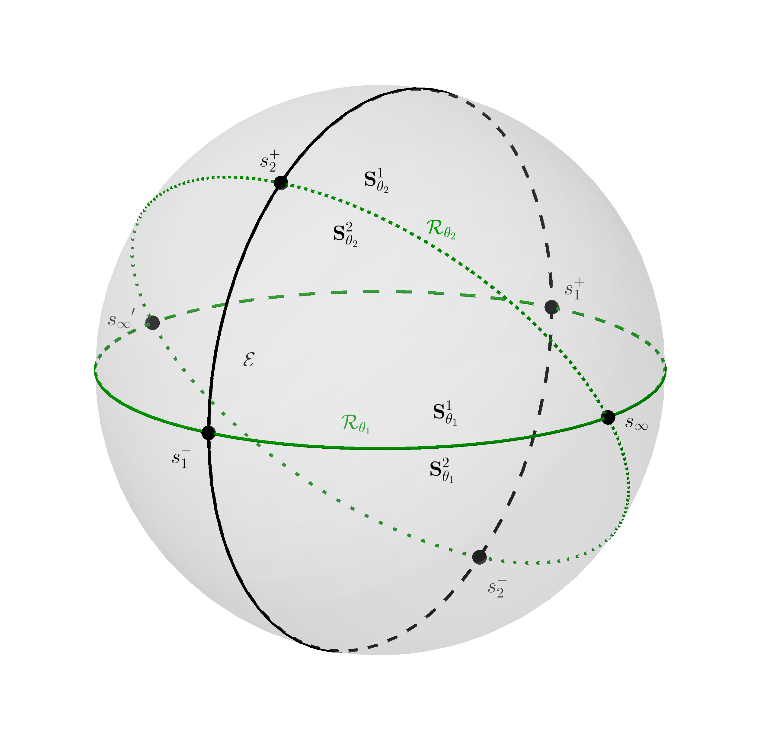
Figure 7. Points of $\mathbf{S}$ with $\theta_{1}(s)$ or $\theta_{2}(s)$ real

2.3. Galois automorphisms $\eta$ and $\zeta$

Now we need to introduce Galois automorphisms on ${\bf S}$. For any $s\in\mathbf{S}\setminus s_{1}^{\pm}$ there is a unique $s^{\prime}\neq s\in\mathbf{S}\setminus s_{1}^{\pm}$ such that $\theta_{1}(s)=\theta_{1}(s^{\prime})$. Furthermore, if $s\in{\mathbf{S}}_{\theta_{1}}^{1}$ then $s^{\prime}\in{\mathbf{S}}_{\theta_{1}}^{2}$ and vice versa. On the other hand, whenever $s=s_{1}^{-}$ or $s=s_{1}^{+}$ (i.e. $\theta_{1}(s)=\theta_{1}^{\pm}$ is one of branch points of $\Theta_{2}(\theta_{1})$) we have $s=s^{\prime}$. Also, since $\gamma(\theta_{1}(s),\theta_{2}(s))=0$, $\theta_{2}(s)$ and $\theta_{2}(s^{\prime})$ represent both values of function $\Theta_{2}(\theta_{1})$ at $\theta_{1}=\theta_{1}(s)=\theta_{1}(s^{\prime})$. By Vieta’s theorem we obtain $\theta_{2}(s)\theta_{2}(s^{\prime})=\frac{c(\theta_{1}(s))}{a(\theta_{1}(s))}$.

Similarly, for any $s\in\mathbf{S}\setminus s_{2}^{\pm}$, there exists a unique $s^{\prime\prime}\neq s\in\mathbf{S}\setminus s_{2}^{\pm}$ such that $\theta_{2}(s)=\theta_{2}(s^{\prime\prime})$. If $s\in{\mathbf{S}}_{\theta_{2}}^{1}$ then $s^{\prime}\in{\mathbf{S}}_{\theta_{2}}^{2}$ and vice versa. On the other hand, if $s=s_{2}^{-}$ or $s=s_{2}^{+}$ (i.e. $\theta_{2}(s)=\theta_{2}^{\pm}$ is one of branch points of $\Theta_{1}(\theta_{2})$) we have $s=s^{\prime\prime}$. Moreover, since $\gamma(\theta_{1}(s),\theta_{2}(s))=0$, $\theta_{1}(s)$ and $\theta_{1}(s^{\prime\prime})$ give both values of function $\Theta_{1}(\theta_{2})$ at $\theta_{2}=\theta_{2}(s)=\theta_{2}(s^{\prime\prime})$. Again, by Vieta’s theorem $\theta_{1}(s)\theta_{1}(s^{\prime\prime})=\frac{\tilde{c}(\theta_{2}(s))}{\tilde{a}(\theta_{2}(s))}$.

With the previous notations we now define the mappings $\zeta:\mathbf{S}\to\mathbf{S}$ and $\eta:\mathbf{S}\to\mathbf{S}$ by

$\left\{\begin{tabular}[]{cc}$\zeta s=s^{\prime}$&if $\theta_{1}(s)=\theta_{1}(s^{\prime})$,\\ $\eta s=s^{\prime\prime}$&if $\theta_{2}(s)=\theta_{2}(s^{\prime\prime})$\\ \end{tabular}\right.$

Following [35] we call them Galois automorphisms of $\mathbf{S}$. Then $\zeta^{2}=\eta^{2}=\text{Id}$, and

$\theta_{2}(\zeta s)=\frac{c(\theta_{1}(s))}{a(\theta_{1}(s))}\frac{1}{\theta_{2}(s)}$,

$\theta_{1}(\eta s)=\frac{\tilde{c}(\theta_{2}(s))}{\tilde{a}(\theta_{2}(s))}\frac{1}{\theta_{1}(s)}$.

Points $s_{1}^{-}$ and $s_{1}^{+}$ (resp. $s_{2}^{-}$ and $s_{2}^{+}$) are fixed points for $\zeta$ (resp. $\eta$).

It is known that conformal automorphisms of a sphere (that can be identified to ${\bf C}\cup\infty$) are transformations of type $z\mapsto\frac{az+b}{cz+d}$ where $a,b,c,d$ are any complex numbers satisfying $ad-bc\neq 0$. The automorphisms $\zeta$ and $\eta$, which are conformal automorphisms of $\mathbf{S}$, have each two fixed points and are involutions (because $\zeta^{2}=\eta^{2}=\text{Id}$). We can deduce from it that $\zeta$ (resp. $\eta$) is a symmetry w.r.t. the axis $A_{1}$ (resp. $A_{2}$) that passes through fixed points $s_{1}^{-}$ and $s_{1}^{+}$ (resp. $s_{2}^{-}$ and $s_{2}^{+}$). In other words $\zeta$ (resp. $\eta$) is a rotation of angle $\pi$, around $D_{1}$ (resp. $A_{2}$), see Figure 8. Let us draw the axis $A$ orthogonal to the plane generated by the axes $A_{1}$ and $A_{2}$ and passing through the intersection point of $A_{1}$ and $A_{2}$. We denote by $\beta$ the angle between the axes $A_{1}$ and $A_{2}$. Automorphisms $\eta\zeta$ and $\zeta\eta$ are then rotations of angle $2\beta$ and $-2\beta$ around the axis $A$. This axis goes through points $s_{\infty}$ and $s_{\infty\prime}$ which are fixed points for $\eta\zeta$ and $\zeta\eta$, see Figure 8.

In the particular case $\Sigma=\text{Id}$, we have $\eta\zeta=\zeta\eta$, the axes $A_{1}$ and $A_{2}$ are orthogonal. We deduce that $\beta=\frac{\pi}{2}$ and that $\eta\zeta$ and $\zeta\eta$ are symmetries w.r.t. the axis $A$.

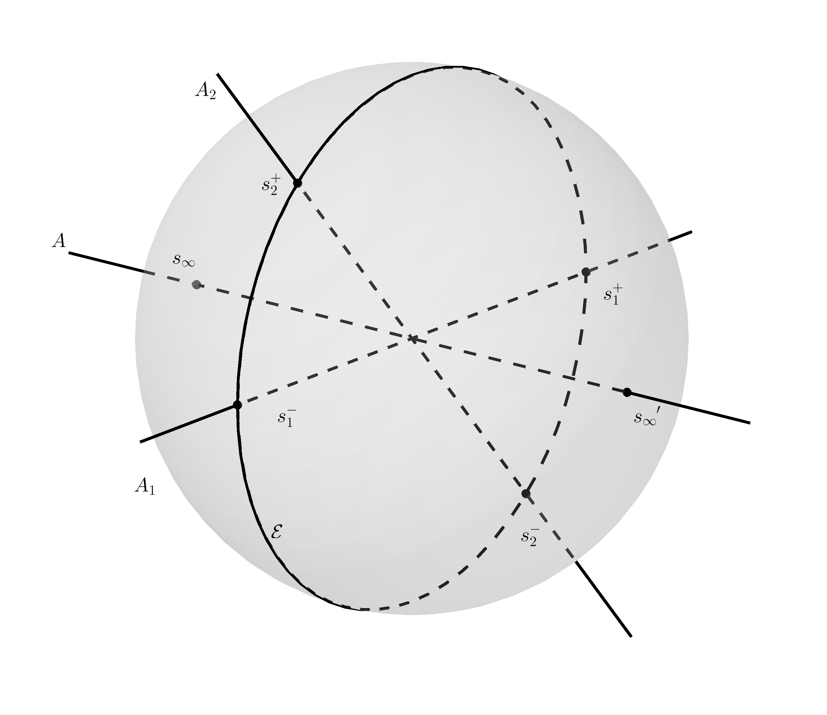
Figure 8. Axes $A_{1}$, $A_{2}$ and $A$ of Galois automorphisms $\zeta$, $\eta$ and $\zeta\eta$ respectively

2.4. Domains of initial definition of $\varphi_{1}$ and $\varphi_{2}$ on ${\bf S}$

We would like to lift functions $\varphi_{1}(\theta_{2})$ and $\varphi_{2}(\theta_{1})$ on ${\bf S}$ naturally as $\varphi_{1}(s)=\varphi_{1}(\theta_{2}(s))$ and $\varphi_{2}(s)=\varphi_{2}(\theta_{1}(s))$. But it can not be done for all $s\in{\bf S}$, $\varphi_{1}(\theta_{2})$ and $\varphi_{2}(\theta_{1})$ being not defined on the whole of ${\bf C}$. Nevertheless, we are able to do it for points $s$ where $\theta_{2}(s)$ or $\theta_{1}(s)$ respectively have non-positive real parts. Therefore, in this section we study the domains on ${\bf S}$ where it holds true.

For any $\theta_{1}\in{\bf C}$ with ${\mathcal{R}}(\theta_{1})=0$, $\Theta_{2}(\theta_{1})$ takes two values $\Theta_{2}^{\pm}(\theta_{1})$. Let us observe that under assumption that the second coordinate of the interior drift is negative, i.e  $\mu_{2}<0$ we have ${\mathcal{R}}\Theta_{2}^{-}(\theta_{1})\leqslant 0$ and ${\mathcal{R}}\Theta_{2}^{+}(\theta_{1})>0$. Furthermore ${\mathcal{R}}\Theta_{2}^{-}(\theta_{1})=0$ only at $\theta_{1}=0$, and then $\Theta_{2}^{-}(\theta_{1})=0$. The domain

$$\Delta_{1}=\{s\in\mathbf{S}:\ {\mathcal{R}}\theta_{1}(s)<0\}$$

is simply connected and bounded by the contour $\mathcal{I}_{\theta_{1}}=\{s:{\mathcal{R}}\theta_{1}(s)=0\}$.

The contour $\mathcal{I}_{\theta_{1}}$ can be represented as the union of $\mathcal{I}_{\theta_{1}}^{-}\cup\mathcal{I}_{\theta_{1}}^{+}$ , where $\mathcal{I}_{\theta_{1}}^{-}=\{s:{\mathcal{R}}\theta_{1}(s)=0,{\mathcal{R}}\theta_{2}(s)\leqslant 0\}$, $\mathcal{I}_{\theta_{1}}^{+}=\{s:{\mathcal{R}}\theta_{1}(s)=0,{\mathcal{R}}\theta_{2}(s)>0\}$, see Figure 9.

The contour $\mathcal{I}_{\theta_{1}}^{-}$ goes from $s_{\infty}$ to $s_{\infty\prime}$ crossing the set of real points $\mathcal{E}$ at $s_{0}=(0,0)$, while $\mathcal{I}_{\theta_{1}}^{+}$ goes from $s_{\infty}$ to $s_{\infty\prime}$ crossing $\mathcal{E}$ at $s^{\prime}_{0}=(0,-2\frac{\mu_{2}}{\sigma_{22}})$ where the second coordinate is positive.

In the same way, under assumption that the first coordinate of the interior drift is negative, i.e. $\mu_{1}<0$, for any $\theta_{2}\in{\bf C}$ with ${\mathcal{R}}(\theta_{2})=0$, $\Theta_{1}(\theta_{2})$ takes two values $\Theta_{1}^{\pm}(\theta_{2})$, where ${\mathcal{R}}\Theta_{1}^{-}(\theta_{2})\leqslant 0$ and ${\mathcal{R}}\Theta_{1}^{+}(\theta_{2})>0$, moreover ${\mathcal{R}}\Theta_{1}^{-}(\theta_{2})=0$ only at $\theta_{2}=0$, and then $\Theta_{1}^{-}(\theta_{2})=0$. The domain

$$\Delta_{2}=\{s\in\mathbf{S}:{\mathcal{R}}\theta_{2}(s)<0\}$$

is simply connected and bounded by the contour $\mathcal{I}_{\theta_{2}}=\{s:{\mathcal{R}}\theta_{2}(s)=0\}$. The contour $\mathcal{I}_{\theta_{2}}$ can be represented as the union of $\mathcal{I}_{\theta_{2}}^{-}\cup\mathcal{I}_{\theta_{2}}^{+}$ , where $\mathcal{I}_{\theta_{2}}^{-}=\{s:{\mathcal{R}}\theta_{2}(s)=0,{\mathcal{R}}\theta_{1}(s)\leqslant 0\}$, $\mathcal{I}_{\theta_{2}}^{+}=\{s:{\mathcal{R}}\theta_{2}(s)=0,{\mathcal{R}}\theta_{1}(s)>0\}$. The contour $\mathcal{I}_{\theta_{2}}^{-}$ goes from $s_{\infty}$ to $s_{\infty\prime}$ crossing the set of real points $\mathcal{E}$ at $s_{0}=(0,0)$, while $\mathcal{I}_{\theta_{2}}^{+}$ goes from $s_{\infty}$ to $s_{\infty\prime}$ crossing $\mathcal{E}$ at $s^{\prime\prime}_{0}=(-2\frac{\mu_{1}}{\sigma_{11}},0)$, see Figure 9.

Assume now that the interior drift has both coordinates negative, i.e. (6). From what said above, $\mathcal{I}_{\theta_{1}}^{-}\setminus s_{0}\subset\Delta_{2}$ and $\mathcal{I}_{\theta_{2}}^{-}\setminus s_{0}\subset\Delta_{1}$. The intersection $\Delta_{1}\cap\Delta_{2}$ consists of two connected components, both bounded by $\mathcal{I}_{\theta_{1}}^{-}$ and $\mathcal{I}_{\theta_{2}}^{-}$. The union $\Delta_{1}\cup\Delta_{2}$ is a connected domain, but not simply connected because of the point $s_{0}$. The domain $\Delta_{1}\cup\Delta_{2}\cup s_{0}$ is open, simply connected and bounded by $\mathcal{I}_{\theta_{1}}^{+}$ and $\mathcal{I}_{\theta_{2}}^{+}$, see Figure 9. We set $\Delta=\Delta_{1}\cup\Delta_{2}$.

Note that in the cases of stationary SRBM with drift $\mu$ having one of coordinates non-negative, the location of contours $\mathcal{I}_{\theta_{1}}^{+}$, $\mathcal{I}_{\theta_{1}}^{-}$, $\mathcal{I}_{\theta_{2}}^{+}$, $\mathcal{I}_{\theta_{2}}^{-}$ on ${\bf S}$ is different. For example, assume that $\mu_{2}>0$. Then ${\mathcal{R}}\Theta_{2}^{-}(\theta_{1})<0$ and ${\mathcal{R}}\Theta_{2}^{+}(\theta_{1})\geqslant 0$, the contour $\mathcal{I}_{\theta_{1}}^{-}$ goes from $s_{\infty}$ to $s_{\infty\prime}$ crossing the set of real points $\mathcal{E}$ at $s^{\prime}_{0}=(0,-2\frac{\mu_{2}}{\sigma_{22}})$ where the second coordinate is negative, while $\mathcal{I}_{\theta_{1}}^{+}$ goes from $s_{\infty}$ to $s_{\infty\prime}$ crossing $\mathcal{E}$ at $s_{0}=(0,0)$. In order to shorten the number of cases and pictures, we restrict ourselves in this paper to the case (6) of both coordinates of $\mu$ negative, although all our methods work in these other cases as well.

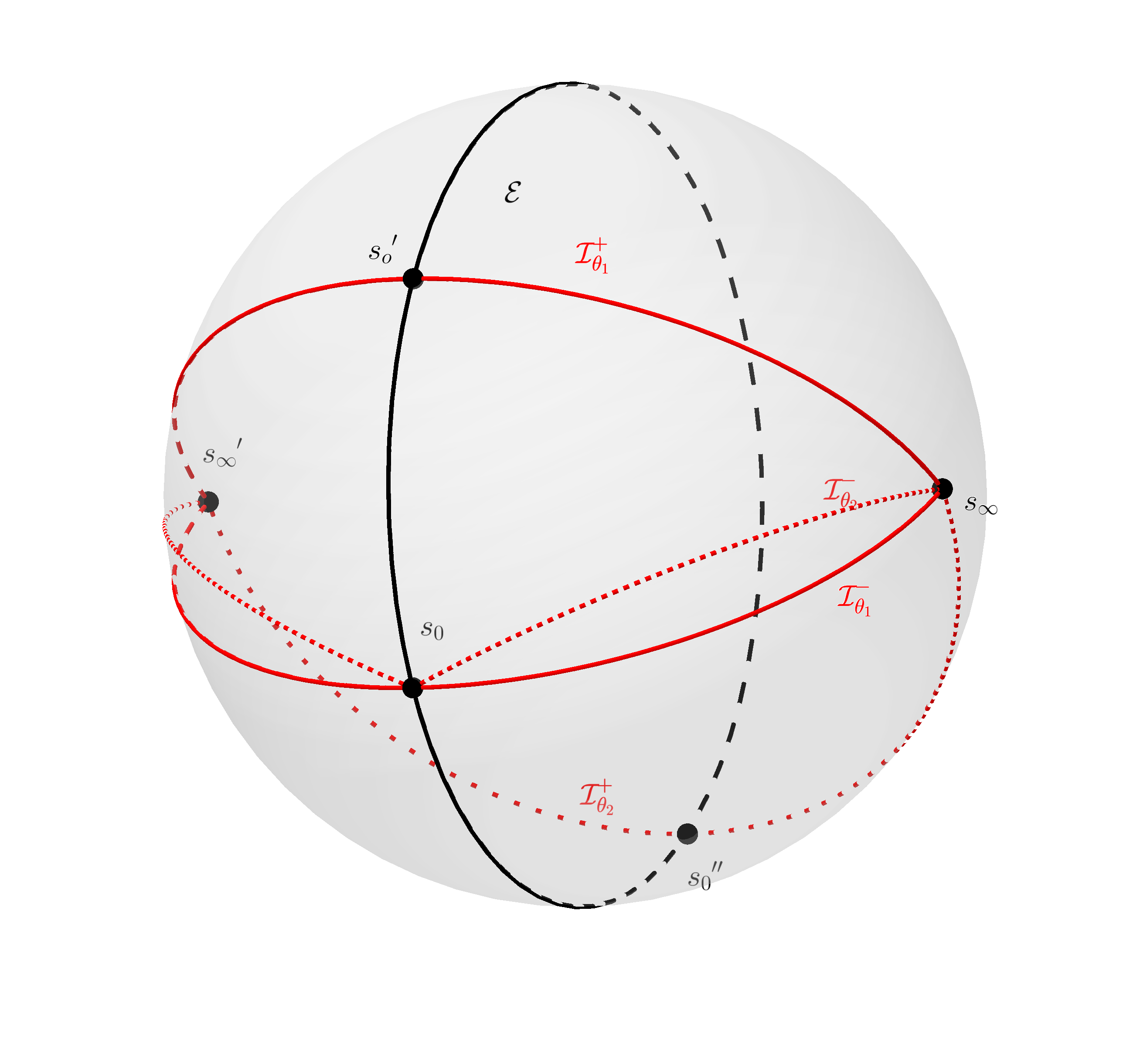
Figure 9. Pure imaginary points of $\mathbf{S}$

2.5. Parametrization of $\mathbf{S}$

It is difficult to visualize on three-dimensional sphere different points, contours, automorphisms and domains introduced above that will be used in future steps. For this reason we propose here an explicit and practical parametrisation of $\mathbf{S}$. Namely we identify $\mathbf{S}$ to $\mathbb{C}\cup\{\infty\}$ and in the next proposition we explicitly define $h_{\theta_{1}}$ and $h_{\theta_{2}}$ two recoveries introduced in Section 2.2. Such a parametrisation allows to visualize better in two dimensions the sphere $\mathbf{S}\equiv\mathbb{C}\cup\{\infty\}$ and all sets we are interested in, as we can see in Figure 10.

Proposition 5.

We set the following covering maps

$$\begin{array}[]{lrcl}h_{\theta_{1}}:&\mathbb{C}\cup\{\infty\}\equiv\mathbf{S}&\longrightarrow&\mathbb{C}\cup\{\infty\}\\ &s&\longmapsto&h_{\theta_{1}}(s)=\theta_{1}(s):=\frac{\theta_{1}^{+}+\theta_{1}^{-}}{2}+\frac{\theta_{1}^{+}-\theta_{1}^{-}}{4}(s+\frac{1}{s})\end{array}$$

and

$$\begin{array}[]{lrcl}h_{\theta_{2}}:&\mathbb{C}\cup\{\infty\}\equiv\mathbf{S}&\longrightarrow&\mathbb{C}\cup\{\infty\}\\ &s&\longmapsto&h_{\theta_{2}}(s)=\theta_{2}(s):=\frac{\theta_{2}^{+}+\theta_{2}^{-}}{2}+\frac{\theta_{2}^{+}-\theta_{2}^{-}}{4}(\frac{s}{e^{i\beta}}+\frac{e^{i\beta}}{s}),\end{array}$$

where

$$\beta=\arccos{-\frac{\sigma_{12}}{\sqrt{\sigma_{11}\sigma_{22}}}}.$$

The equation $\gamma(\theta_{1}(s),\theta_{2}(s))=0$ is valid for any $s\in\mathbf{S}$. Galois automorphisms can be written

$\zeta(s)=\frac{1}{s}$,

$\eta(s)=\frac{e^{2i\beta}}{s}$,

and $\eta\zeta$ (resp. $\zeta\eta$) is a rotation around $s_{\infty}\equiv 0$ of angle $2\beta$ (resp. $-2\beta$) according to counterclockwise direction.

Proof.

We set $h_{\theta_{1}}(s)=\theta_{1}(s):=\frac{\theta_{1}^{+}+\theta_{1}^{-}}{2}+\frac{\theta_{1}^{+}-\theta_{1}^{-}}{4}(s+\frac{1}{s})$. One can notice that $h_{\theta_{1}}(1)=\theta_{1}^{+}$, $h_{\theta_{1}}(-1)=\theta_{1}^{-}$, $h_{\theta_{1}}^{\prime}(1)=0$, $h_{\theta_{1}}^{\prime}(-1)=0$. This parametrization is practical because it leads to a similar rational recovery $h_{\theta_{2}}$. In order to make the equation $\gamma(\theta_{1}(s),\theta_{2}(s))=0$ valid for any $s\in\mathbf{S}$ we naturally set

$$\theta_{2}(s)=\Theta_{2}^{+}(\theta_{1}(s)):=\frac{-b(\theta_{1}(s))+\sqrt{d(\theta_{1}(s))}}{2a(\theta_{1}(s))}$$

and we are going to show that $\theta_{2}(s)=\frac{\theta_{2}^{+}+\theta_{2}^{-}}{2}+\frac{\theta_{2}^{+}-\theta_{2}^{-}}{4}(\frac{s}{e^{i\beta}}+\frac{e^{i\beta}}{s})$ where $\beta=\arccos{-\frac{\sigma_{12}}{\sqrt{\sigma_{11}\sigma_{22}}}}$. We note that $d(\theta_{1}(s))$ is the opposite of the square of a rational fraction

$$d(\theta_{1}(s)) =-\det\Sigma(\theta_{1}(s)-\theta_{1}^{+})(\theta_{1}(s)-\theta_{1}^{-})=-\det\Sigma(\frac{\theta_{1}^{+}-\theta_{1}^{-}}{4})^{2}(-2+(s+\frac{1}{s}))(2+(s+\frac{1}{s}))$$

$$=-\det\Sigma(\frac{\theta_{1}^{+}-\theta_{1}^{-}}{4})^{2}(s-\frac{1}{s})^{2}\leqslant 0.$$

Then we have

$$\theta_{2}(s)=\Theta_{2}^{+}(\theta_{1}(s)):=\frac{-\sigma_{12}\frac{\theta_{1}^{+}+\theta_{1}^{-}}{2}+\frac{\theta_{1}^{+}-\theta_{1}^{-}}{4}(s+\frac{1}{s})-\mu_{2}+i\sqrt{\det\Sigma}(\frac{\theta_{1}^{+}-\theta_{1}^{-}}{4})(s-\frac{1}{s})}{\sigma_{22}}.$$ (14)

Furthermore this parametrization leads to simple expressions for Galois automorphisms $\eta$ and $\zeta$. We derive immediately that $\theta_{1}(s)=\theta_{1}(\frac{1}{s})$ and $\theta_{2}(\frac{1}{s})=\Theta_{2}^{-}(\theta_{1}(s))$. Then we have

$$\zeta(s)=\frac{1}{s}.$$

Next we search $\eta$ as an automorphism of the form $\eta s=\frac{K}{s}$. Since $\theta_{2}(s)$ is of the form $\theta_{2}(s)=us+\frac{v}{s}+w$ with constants $u,v,w$ defined by (14), then $\theta_{2}(s)=\theta_{2}(\frac{K}{s})$ with $K=\frac{u}{v}$. This leads to

$$\eta(s)=\frac{K}{s}\text{ with }K=\frac{-\sigma_{12}-i\sqrt{\det\Sigma}}{-\sigma_{12}+i\sqrt{\det\Sigma}}.$$

After setting

$$K=e^{2i\beta}\text{ with }\beta=\arccos{-\frac{\sigma_{12}}{\sqrt{\sigma_{11}\sigma_{22}}}}$$

we have

${\zeta}(s)=\frac{1}{s}$,

${\eta}(s)=\frac{e^{2i\beta}}{s}$

and then

$\eta\zeta(s)=e^{2i\beta}s$,

$\zeta\eta(s)=e^{-2i\beta}s$.

It follows that ${\eta}{\zeta}$ and ${\zeta}{\eta}$ are just rotations for angles $2\beta$ et $-2\beta$ respectively. By symmetry considerations we can now rewrite

$$\theta_{2}(s)=\sqrt{uv}(\frac{s}{\sqrt{K}}+\frac{\sqrt{K}}{s})+w=\frac{\theta_{1}^{+}-\theta_{1}^{-}}{4}\sqrt{\frac{\sigma_{11}}{\sigma_{22}}}(\frac{s}{\sqrt{K}}+\frac{\sqrt{K}}{s})+\frac{-\sigma_{12}(\frac{\theta_{1}^{+}+\theta_{1}^{-}}{2})-\mu_{2}}{\sigma_{22}}.$$

For $i=1,2$ we have $\theta_{i}^{+}-\theta_{i}^{-}=2\frac{\sqrt{D_{i}}}{\det\Sigma}$ and $\sigma_{11}D_{1}=\sigma_{22}D_{2}$. Then we obtain $\frac{\theta_{1}^{+}-\theta_{1}^{-}}{4}\sqrt{\frac{\sigma_{11}}{\sigma_{22}}}=\frac{\theta_{2}^{+}-\theta_{2}^{-}}{4}$. Moreover $\frac{-\sigma_{12}(\frac{\theta_{1}^{+}+\theta_{1}^{-}}{2})-\mu_{2}}{\sigma_{22}}=\frac{\Theta_{2}^{\pm}(\theta_{1}^{+})+\Theta_{2}^{\pm}(\theta_{1}^{-})}{2}=\frac{\theta_{2}^{+}+\theta_{2}^{-}}{2}$ (the last equality follows from elementary geometric properties of an ellipse). It implies

$$h_{\theta_{2}}(s)=\theta_{2}(s)=\frac{\theta_{2}^{+}+\theta_{2}^{-}}{2}+\frac{\theta_{2}^{+}-\theta_{2}^{-}}{4}(\frac{s}{\sqrt{K}}+\frac{\sqrt{K}}{s})$$

concluding the proof. ∎

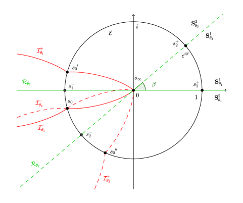
Figure 10. Parametrization of $\mathbf{S}$

Figure 10 shows different sets we are interested in according to the parametrization we have just introduced. We have $\theta_{1}(1)=\theta_{1}^{+}$, $\theta_{1}(-1)=\theta_{1}^{-}$, $\theta_{2}(e^{i\beta})=\theta_{2}^{+}$ et $\theta_{2}(e^{i(\pi+\beta)})=\theta_{2}^{-}$, $\theta_{1}(0)=\theta_{2}(0)=\infty$, $\theta_{1}(\infty)=\theta_{2}(\infty)=\infty$. Then we write $s_{1}^{+}=1$, $s_{1}^{-}=-1$, $s_{2}^{+}=e^{i\beta}$, $s_{2}^{-}=e^{i(\pi+\beta)}$, $s_{\infty}=0$, $s_{\infty^{\prime}}=\infty$. It is easy to see that

$$\mathcal{E}=\{s\in\mathbb{C}|\ |s|=1\},$$

and

$$\mathcal{R}_{\theta_{1}}={\bf R},\ \mathcal{R}_{\theta_{2}}=e^{i\beta}{\bf R}.$$

We can determine the equation of the analytic curves of pure imaginary points of $\theta_{i}$. We have ${\mathcal{I}}_{\theta_{1}}=\{s\in\mathbf{S}|\theta_{1}(s)\in i{\bf R}\}$. If we write $s=e^{i\omega}$ with $\omega=a+ib\in\mathbb{C}$ we find that $\Re(\theta_{1}(s))=\frac{\theta_{1}^{+}+\theta_{1}^{-}}{2}+\frac{\theta_{1}^{+}-\theta_{1}^{-}}{2}\cos(a)\cosh(b)$. It follows that

$${\mathcal{I}}_{\theta_{1}}=\{s=e^{i\omega}\in\mathbf{S}|\omega=a+ib,a\in{\bf R},b\in{\bf R},\cos(a)\cosh(b)=\frac{\theta_{1}^{+}+\theta_{1}^{-}}{\theta_{1}^{-}-\theta_{1}^{+}}\}.$$

Similarly we have

$${\mathcal{I}}_{\theta_{2}}=\{s=e^{i\omega}\in\mathbf{S}|\omega=a+ib,a\in{\bf R},b\in{\bf R},\cos(a)\cosh(b)=\frac{\theta_{2}^{+}+\theta_{2}^{-}}{\theta_{2}^{-}-\theta_{2}^{+}}\}.$$

We can easily notice that

$${\zeta}{\mathcal{I}}_{\theta_{1}}^{-}={\mathcal{I}}_{\theta_{1}}^{+},\ {\zeta}{\mathcal{I}}_{\theta_{1}}^{+}={\mathcal{I}}_{\theta_{1}}^{-}\text{ and }{\eta}{\mathcal{I}}_{\theta_{2}}^{-}={\mathcal{I}}_{\theta_{2}}^{+},\ {\eta}{\mathcal{I}}_{\theta_{2}}^{+}={\mathcal{I}}_{\theta_{2}}^{-}.$$

3. Meromorphic continuation of $\varphi_{1}$ and $\varphi_{2}$ on $\mathbf{S}$

3.1. Lifting of $\varphi_{1}$ and $\varphi_{2}$ on $\mathbf{S}$ and their meromomorphic continuation

Lifting of $\varphi_{1}$ and $\varphi_{2}$ on $\mathbf{S}$.

Since the function $\theta_{1}\to\varphi_{2}(\theta_{1})$ is holomorphic on the set $\{\theta_{1}\in\mathbb{C}:\Re\theta_{1}<0\}$ and continuous up to its boundary, we can lift it to $\bar{\Delta}_{1}=\{s\in\mathbf{S}:\Re\theta_{1}(s)\leqslant 0\}$ as

$$\varphi_{2}(s)=\varphi_{2}(\theta_{1}(s)),\ \forall s\in\bar{\Delta}_{1}.$$

In the same way we can lift $\varphi_{1}$ to $\bar{\Delta}_{2}$ as

$$\varphi_{1}(s)=\varphi_{1}(\theta_{2}(s)),\ \forall s\in\bar{\Delta}_{2}.$$

Moreover, by definition of Galois automorphisms, functions $\varphi_{1}$ and $\varphi_{2}$ are invariant w.r.t. $\eta$ and $\zeta$ respectively:

$$\varphi_{2}(\zeta s)=\varphi_{2}(\theta_{1}(\zeta s))=\varphi_{2}(\theta_{1}(s))=\varphi_{2}(s),\ \ \forall s\in\bar{\Delta}_{1},$$

$$\varphi_{1}(\eta s)=\varphi_{1}(\theta_{2}(\eta s))=\varphi_{1}(\theta_{2}(s))=\varphi_{1}(s),\ \ \forall s\in\bar{\Delta}_{2}.$$ (15)

Functions $\gamma_{1}$ and $\gamma_{2}$ can be lifted naturally on the whole of ${\bf S}$ as

$$\gamma_{1}(s)=\gamma_{1}(\theta_{1}(s),\theta_{2}(s)),\ \ \ \ \gamma_{2}(s)=\gamma_{2}(\theta_{1}(s),\theta_{2}(s))\ \ \ \forall s\in{\bf S}.$$

Since $\gamma(\theta_{1}(s),\theta_{2}(s))=0$, then the right-hand side in the main functional equation (4) equals zero for any $\theta=(\theta_{1}(s),\theta_{2}(s))$ such that $s\in\bar{\Delta}_{1}\cap\bar{\Delta}_{2}$. Thus we have

$$\gamma_{1}(s)\varphi(s)+\gamma_{2}(s)\varphi_{2}(s)=0,\ \ \ \forall s\in\bar{\Delta}_{1}\cap\bar{\Delta}_{2}.$$ (16)

Continuation of $\varphi_{1}$ and $\varphi_{2}$ on $\Delta$.

Lemma 6.

Functions $\varphi_{1}$ and $\varphi_{2}$ (defined on $\bar{\Delta}_{2}$ and $\bar{\Delta}_{1}$ respectively) can be meromorphically continued on $\Delta\cup\{s_{0}\}$ by setting

$$\varphi_{1}(s)=\begin{tabular}[]{cc}$-\frac{\gamma_{2}(s)}{\gamma_{1}(s)}\varphi_{2}(s)$&if $s\in\Delta_{1},$\\ \end{tabular}$$

and

$$\varphi_{2}(s)=\begin{tabular}[]{cc}$-\frac{\gamma_{1}(s)}{\gamma_{2}(s)}\varphi_{1}(s)$&if $s\in\Delta_{2}.$\\ \end{tabular}$$

Furthermore,

$$\gamma_{1}(s)\varphi_{1}(s)+\gamma_{2}(s)\varphi_{2}(s)=0\ \ \forall s\in\Delta\cup\{s_{0}\},$$ (17)

$$\varphi_{1}(s)=\varphi(\eta s),\ \ \ \ \varphi_{2}(s)=\varphi(\zeta s)\ \ \forall s\in\Delta\cup\{s_{0}\}.$$ (18)

Proof.

The open set $\Delta_{1}\cap\Delta_{2}$ is non-empty and bounded by the curve $\mathcal{I}_{\theta_{1}}^{-}\cup\mathcal{I}_{\theta_{2}}^{-}$. Functional equation (16) is valid for $s\in\Delta_{1}\cap\Delta_{2}$. It allows us to continue functions $\varphi_{1}$ and $\varphi_{2}$ as meromorphic on $\Delta$ as stated in this lemma. The functional equation (16) is then valid on the whole of $\Delta$, as well as the invariance formulas (18). ∎

The function $\varphi_{1}(s)$ is defined in a neighborhood $\mathcal{O}(s_{0})$ of $s_{0}$ as $\varphi_{1}(\theta_{2}(s))$ for any $s\in\Delta_{2}\cap\mathcal{O}(s_{0})$ and $-\frac{\gamma_{2}(s)}{\gamma_{1}(s)}\varphi_{2}(\theta_{1}(s))$ for any $s\in\Delta_{1}\cap\mathcal{O}(s_{0})$. Furthermore,

$$\lim_{s\to s_{0},s\in\Delta_{2}}\varphi_{1}(s)=\mathbb{E}_{\pi}(\int_{0}^{1}\mathrm{d}L_{t}^{1})$$

by definition of the function $\varphi_{1}.$ It is easy to see that function $\frac{\gamma_{2}(s)}{\gamma_{1}(s)}$ has a removable singularity at $s_{0}$ and to compute $\lim_{s\to s_{0}}\frac{\gamma_{2}(s)}{\gamma_{1}(s)}=\frac{r_{12}\mu_{2}-r_{22}\mu_{1}}{r_{11}\mu_{2}-r_{21}\mu_{1}}$. Hence

$$\lim_{s\to s_{0},s\in\Delta_{1}}\varphi_{1}(s)=\lim_{s\to s_{0},s\in\Delta_{1}}-\frac{\gamma_{2}(s)}{\gamma_{1}(s)}\varphi_{2}(\theta_{1}(s))=\frac{r_{22}\mu_{1}-r_{12}\mu_{2}}{r_{11}\mu_{2}-r_{21}\mu_{1}}\mathbb{E}_{\pi}(\int_{0}^{1}\mathrm{d}L_{t}^{2}).$$

For any $s\in\Delta_{1}\cap\Delta_{2}\cap\mathcal{O}(s_{0})$, by (16) $\varphi_{1}(s)=-\frac{\gamma_{2}(s)}{\gamma_{1}(s)}\varphi_{2}(s)$, from where $\lim_{s\to s_{0},s\in\Delta_{2}}\varphi_{1}(s)=\lim_{s\to s_{0},s\in\Delta_{1}}\varphi_{1}(s)$. Hence, function $\varphi_{1}(s)$ has a removable singularity at $s_{0}$, and so is $\varphi_{2}(s)$ by the same arguments.

Functions $\varphi_{1}$ and $\varphi_{2}$ can be then of course continued to $\bar{\Delta}$. Moreover we have the following lemma.

Lemma 7.

The domains $\bar{\Delta}\cup\eta\zeta\bar{\Delta}$ and $\bar{\Delta}\cup\zeta\eta\bar{\Delta}$ are simply connected.

Proof.

Since $\eta\zeta$ and $\zeta\eta$ are just rotations for a certain angle $2\beta$ or $-2\beta$, it suffices to check that $\eta\zeta\mathcal{I}_{\theta_{1}}^{+}\subset\bar{\Delta}$ and that $\zeta\eta\mathcal{I}_{\theta_{2}}^{+}\in\bar{\Delta}$. In fact, $\zeta\mathcal{I}_{\theta_{1}}^{+}=\mathcal{I}_{\theta_{1}}^{-}\subset\bar{\Delta}_{2}.$ Since $\eta\bar{\Delta}_{2}=\bar{\Delta}_{2}$, it follows that $\eta\mathcal{I}_{\theta_{1}}^{-}\subset\bar{\Delta}_{2}\subset\bar{\Delta}$. By the same arguments $\zeta\eta\mathcal{I}_{\theta_{2}}^{+}\in\bar{\Delta}$. One can refer to Figure 11. ∎

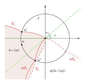
Figure 11. $\Delta$ and $\eta\zeta\Delta$

Now we would like to continue function $\varphi_{1}$ (resp. $\varphi_{2}$) on $\eta\zeta\bar{\Delta}$ (resp. $\zeta\eta\bar{\Delta}$) as $\varphi_{1}(s)=G(s)\varphi_{1}(\zeta\eta s)$ for all $s\in\eta\zeta\bar{\Delta}$, where $G(s)$ is a known function and $\varphi_{1}(\zeta\eta s)$ is well defined since $\zeta\eta s\in\bar{\Delta}$. We could then continue this procedure for $(\eta\zeta)^{2}\bar{\Delta}$, $(\eta\zeta)^{3}\bar{\Delta}$, (resp. $(\zeta\eta)^{2}\bar{\Delta}$, $(\zeta\eta)^{3}\bar{\Delta}$) etc and hence to define $\varphi_{1}$ (resp. $\varphi_{2}$) on the whole of ${\bf S}$. Unfortunately, the domain $\bar{\Delta}$ is closed, from where it will be difficult to establish that the function is meromorphic. From the other hand, neither $\Delta\cup\eta\zeta\Delta$ nor $(\Delta\cup s_{0})\cup\eta\zeta(\Delta\cup s_{0})$ are simply connected, there is a “gap” at $s^{\prime\prime}_{0}$. See figure 11. To avoid this technical complication, we will first continue $\varphi_{1}$ and $\varphi_{2}$ on a slightly bigger open domain $\Delta^{\epsilon}$ defined as follows. Let

$$\Delta_{1}^{\epsilon}=\{s:{\mathcal{R}}\theta_{1}(s)<\epsilon\},\ \ \ \Delta_{2}^{\epsilon}=\{s:{\mathcal{R}}\theta_{2}(s)<\epsilon\}$$ (19)

and

$$\Delta^{\epsilon}=\Delta_{1}^{\epsilon}\cup\Delta_{2}^{\epsilon}$$ (20)

Let us fix any $\epsilon>0$ small enough. For any $\theta_{1}\in{\bf C}$ with ${\mathcal{R}}\theta_{1}=\epsilon$, the function $\Theta_{2}(\theta_{1})$ takes two values $\Theta_{2}^{\pm}(\theta_{1})$ where ${\mathcal{R}}(\Theta_{2}^{-}(\theta_{1}))<0$ and ${\mathcal{R}}(\Theta_{2}(\theta_{1}))>0$. The domain $\Delta_{1}^{\epsilon}$ is bounded by the contour $\mathcal{I}_{\theta_{1}}^{\epsilon}=\mathcal{I}_{\theta_{1}}^{\epsilon,-}\cup\mathcal{I}_{\theta_{1}}^{\epsilon,+}$ where $\mathcal{I}_{\theta_{1}}^{\epsilon,-}$, $\mathcal{I}_{\theta_{1}}^{\epsilon,+}$ both go from $s_{\infty}$ to $s_{\infty\prime}$, $\mathcal{I}_{\theta_{1}}^{\epsilon,-}\subset\Delta_{2}$ and $\mathcal{I}_{\theta_{1}}^{\epsilon,+}\cap\Delta=\emptyset$. See Figure 12. The same is true about the contour $\mathcal{I}_{\theta_{2}}^{\epsilon}=\mathcal{I}_{\theta_{2}}^{\epsilon,-}\cup\mathcal{I}_{\theta_{2}}^{\epsilon,+}$ limiting $\Delta_{2}^{\epsilon}$, namely $\mathcal{I}_{\theta_{2}}^{\epsilon,-}\subset\Delta_{1}$ and $\mathcal{I}_{\theta_{2}}^{\epsilon,+}\cap\Delta=\emptyset$.

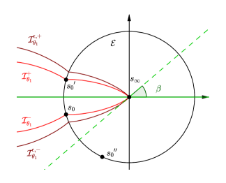
Figure 12. $\mathcal{I}_{\theta_{1}}^{\epsilon,-}$ and $\mathcal{I}_{\theta_{1}}^{\epsilon,+}$

Lemma 8.

Functions $\varphi_{1}(s)$ and $\varphi_{2}(s)$ can be continued as meromorphic functions on $\Delta^{\epsilon}$. Moreover equation (17) and the invariance formulas (18) remain valid.

Proof.

For any $s\in\Delta_{1}^{\epsilon}\setminus\Delta$, we have $\zeta s\in\Delta_{2}\subset\Delta$, except for $s=s^{\prime}_{0}$, for which $\zeta s^{\prime}_{0}=s_{0}$. Anyway, function $\varphi_{2}(s)$ can be continued as meromorphic function on $\Delta_{1}^{\epsilon}/\Delta$ as :

$$\varphi_{2}(s)=\varphi_{2}(\zeta s),\ \ \ \forall s\in\Delta_{1}^{\epsilon}\setminus\Delta.$$

Then $\varphi_{1}(s)$ can be continued on the same domain by (17):

$$\varphi_{1}(s)=-\frac{\gamma_{2}(s)}{\gamma_{1}(s)}\varphi_{2}(s)\ \ \ \forall s\in\Delta_{1}^{\epsilon}\setminus\Delta.$$

Similarly, the formulas

$$\varphi_{1}(s)=\varphi_{1}(\eta s),\ \ \varphi_{2}(s)=-\frac{\gamma_{1}(s)}{\gamma_{2}(s)}\varphi_{1}(s)\ \ \ \forall s\in\Delta_{2}^{\epsilon}\setminus\Delta$$

determine the meromorphic continuation of $\varphi_{1}(s)$ and $\varphi_{2}(s)$ on $\Delta_{2}^{\epsilon}\setminus\Delta$. ∎

Lemma 9.

The domains $\Delta^{\epsilon}\cap\eta\zeta\Delta^{\epsilon}$ and $\Delta^{\epsilon}\cap\zeta\eta\Delta^{\epsilon}$ are open simply connected domains. Function $\varphi_{1}(s)$ can be continued as meromorphic on $\Delta^{\epsilon}\cup\eta\zeta\Delta^{\epsilon}$ by the formula :

$$\varphi_{1}(s)=\frac{\gamma_{1}(\zeta\eta s)\gamma_{2}(\eta s)}{\gamma_{2}(\zeta\eta s)\gamma_{1}(\eta s)}\varphi_{1}(\zeta\eta s),\ \ \forall s\in\eta\zeta\Delta^{\epsilon}\ \hbox{ continuation by rotation of }2\beta.$$ (21)

Function $\varphi_{2}(s)$ can be continued as meromorphic on $\Delta^{\epsilon}\cup\zeta\eta\Delta^{\epsilon}$ by the formula :

$$\varphi_{2}(s)=\frac{\gamma_{2}(\eta\zeta s)\gamma_{1}(\zeta s)}{\gamma_{1}(\eta\zeta s)\gamma_{2}(\zeta s)}\varphi_{2}(\eta\zeta s),\ \ \forall s\in\zeta\eta\Delta^{\epsilon}\hbox{ continuation by rotation of}-2\beta.$$ (22)

Proof.

We have shown in the proof of Lemma 7 that $\eta\zeta\mathcal{I}_{\theta_{1}}^{+}\subset\bar{\Delta}\subset\Delta^{\epsilon}$, and that $\zeta\eta\mathcal{I}_{\theta_{2}}^{+}\subset\bar{\Delta}\subset\Delta^{\epsilon}$. Since $\zeta\eta$ and $\eta\zeta$ are just rotations, this implies that $\Delta^{\epsilon}\cap\eta\zeta\Delta^{\epsilon}$ and $\Delta^{\epsilon}\cap\zeta\eta\Delta^{\epsilon}$ are non-empty open simply connected domains, and that $\Delta^{\epsilon}\cup\eta\zeta\Delta^{\epsilon}$ and $\Delta^{\epsilon}\cup\zeta\eta\Delta^{\epsilon}$ are simply connected.

Let us take $s\in\Delta^{\epsilon}\cap\eta\zeta\Delta^{\epsilon}$. Then $\zeta\eta s\in\Delta^{\epsilon}\cap\zeta\eta\Delta^{\epsilon}$ and we can write by (17)

$$\gamma_{1}(\zeta\eta s)\varphi_{1}(\zeta\eta s)+\gamma_{2}(\zeta\eta s)\varphi_{2}(\zeta\eta s)=0.$$ (23)

Furthermore, we have shown in the proof of Lemma 7 that $\zeta\eta\mathcal{I}_{\theta_{2}}^{+}\in\bar{\Delta}_{1}$. It follows that for all $\epsilon$ small enough $\zeta\eta\mathcal{I}_{\theta_{2}}^{\epsilon,+}\in\Delta_{1}$, and hence $\Delta^{\epsilon}\cap\zeta\eta\Delta^{\epsilon}\subset\Delta_{1}^{\epsilon}$. Since $\zeta\Delta_{1}^{\epsilon}=\Delta_{1}^{\epsilon}$, then $\zeta(\Delta^{\epsilon}\cap\zeta\eta\Delta^{\epsilon})\subset\Delta_{1}^{\epsilon}\subset\Delta_{\epsilon}$. Then $\zeta(\zeta\eta s)=\eta s\in\Delta^{\epsilon}$ and we can write (17) and (18) at this point as well:

$$\gamma_{1}(\eta s)\varphi_{1}(\eta s)+\gamma_{2}(\eta s)\varphi_{2}(\eta s)=0.$$ (24)

$$\varphi_{1}(\eta s)=\varphi_{1}(s)$$ (25)

$$\varphi_{2}(\eta s)=\varphi_{2}(\zeta\eta s).$$ (26)

Combining (25) and (24) we get $\varphi_{1}(s)=-\gamma_{2}(\eta s)\varphi_{2}(\eta s)/\gamma_{1}(\eta s)$ from where by (26)

$$\varphi_{1}(s)=-\frac{\gamma_{2}(\eta s)}{\gamma_{1}(\eta s)}\varphi_{2}(\zeta\eta s).$$ (27)

Due to (23)

$$\varphi_{2}(\zeta\eta s)=-\frac{\gamma_{1}(\zeta\eta s)}{\gamma_{2}(\zeta\eta s)}\varphi_{1}(\zeta\eta s).$$ (28)

Substituting (28) into (27), we obtain the formula (21) valid for any $s\in\Delta^{\epsilon}\cap\eta\zeta\Delta^{\epsilon}$. By principle of analytic continuation this allows to continue $\varphi_{1}$ on $\eta\zeta\Delta^{\epsilon}$ as meromorphic function. The proof is completely analogous for $\varphi_{2}$. ∎

We may now in the same way, using formulas (21) and (22), continue function $\varphi_{1}(s)$ (resp. $\varphi_{2}(s)$) as meromorphic on $(\eta\zeta)^{2}\Delta^{\epsilon}$, $(\eta\zeta)^{3}\Delta^{\epsilon}$ (resp. $(\zeta\eta)^{2}\Delta^{\epsilon}$, $(\zeta\eta)^{3}\Delta^{\epsilon}$) etc proceeding each time by rotation for the angle $2\beta$ [resp. $-2\beta$]. Namely we have the following lemma.

Lemma 10.

For any $n\geqslant 1$ the domains $\Delta^{\epsilon}\cup\eta\zeta\Delta^{\epsilon}\cup\cdots\cup(\eta\zeta)^{n}\Delta^{\epsilon}$ and $\Delta^{\epsilon}\cup\zeta\eta\Delta^{\epsilon}\cup\cdots(\zeta\eta)^{n}\Delta^{\epsilon}$ are open simply connected domains. Function $\varphi_{1}(s)$ can be continued as meromorphic subsequently on $\eta\zeta\Delta^{\epsilon},(\eta\zeta)^{2}\Delta^{\epsilon},\cdots(\eta\zeta)^{n}\Delta^{\epsilon}$ by the formulas :

$$\varphi_{1}(s)=\frac{\gamma_{1}(\zeta\eta s)\gamma_{2}(\eta s)}{\gamma_{2}(\zeta\eta s)\gamma_{1}(\eta s)}\varphi_{1}(\zeta\eta s),\ \ \forall s\in(\eta\zeta)^{k}\Delta^{\epsilon},k=1,2\ldots,n,\ \hbox{ continuation by rotation of }2\beta.$$ (29)

Function $\varphi_{2}(s)$ can be continued as meromorphic on $\zeta\eta\Delta^{\epsilon},(\zeta\eta)^{2}\Delta^{\epsilon},\cdots(\zeta\eta)^{n}\Delta^{\epsilon}$ by the formulas :

$$\varphi_{2}(s)=\frac{\gamma_{2}(\eta\zeta s)\gamma_{1}(\zeta s)}{\gamma_{1}(\eta\zeta s)\gamma_{2}(\zeta s)}\varphi_{2}(\eta\zeta s),\ \ \forall s\in(\zeta\eta)^{k}\Delta^{\epsilon},k=1,2,\ldots n,\hbox{ continuation by rotation of}-2\beta.$$ (30)

Proof.

We proceed by induction on $k=1,2,\ldots n$. For $k=1$, this is the subject of the previous lemma. For any $k=2,\ldots,n$, assume the formula (29) for any $s\in(\eta\zeta)^{k-1}\Delta$. The domain $(\eta\zeta)^{k-1}\Delta^{\epsilon}\cap(\eta\zeta)^{k}\Delta^{\epsilon}=(\eta\zeta)^{k-1}(\Delta^{\epsilon}\cap\eta\zeta\Delta^{\epsilon})$ is a non empty open domain by Lemma 9, $(\eta\zeta)^{k-1}$ being just the rotation for the angle $2(k-1)\beta$. The formula (29) is valid for any $s\in(\eta\zeta)^{k-1}\Delta^{\epsilon}\cap(\eta\zeta)^{k}\Delta^{\epsilon}$ by induction assumption. Hence, by the principle of meromorphic continuation it is valid for any $s\in(\eta\zeta)^{k}\Delta^{\epsilon}$. The same is true for the formula (30). ∎

Proceeding as in Lemma 10 by rotations, we will continue $\varphi_{1}$ soon on the first half of ${\bf S}$, that is ${\bf S}_{\theta_{2}}^{1}$, then the whole of ${\bf S}$ and go further, turning around ${\bf S}$ for the second time, for the third, etc up to infinity. In fact, each time we complete this procedure on one of two halves of ${\bf S}$, we recover a new branch of the function $\varphi_{1}$ as function of $\theta_{2}\in{\bf C}$. So, going back to the complex plane, we continue this function as multivalued and determine all its branches. The same is true for $\varphi_{2}$ if we proceed by rotations in the opposite direction. This procedure could be presented better on the universal covering of ${\bf S}$, but for the purpose of the present paper it is enough to complete it only on one-half of ${\bf S}$, that is to study just the first (main) branch of $\varphi_{1}$ and $\varphi_{2}$. We summarize this result in the following theorem. We recall that ${\bf S}={\bf S}_{\theta_{1}}^{1}\cup{\bf S}_{\theta_{1}}^{2}$ and we denote by ${\bf S}_{\theta_{1}}^{1}$ the half that contains $s^{\prime}_{0}$ (and not $s_{0}$, as $\zeta s_{0}=s^{\prime}_{0}$). In the same way ${\bf S}={\bf S}_{\theta_{2}}^{1}\cup{\bf S}_{\theta_{2}}^{2}$ and we denote by ${\bf S}_{\theta_{2}}^{1}$ the half that contains $s^{\prime\prime}_{0}$ (and not $s_{0}$, as $\eta s_{0}=s^{\prime\prime}_{0}$), see Figure 10.

Theorem 11.

For any $s\in{\bf S}_{\theta_{2}}^{1}$ there exists $n\geqslant 0$ such that $(\zeta\eta)^{n}s\in\bar{\Delta}$. Let us define

$$\varphi_{1}(s)=\frac{\gamma_{1}((\zeta\eta)^{n}s)\dots\gamma_{1}(\zeta\eta s)}{\gamma_{2}((\zeta\eta)^{n}s)\dots\gamma_{2}(\zeta\eta s)}\frac{\gamma_{2}(\eta(\zeta\eta)^{n-1}s)\dots\gamma_{2}(\eta s)}{\gamma_{1}(\eta\zeta\eta)^{n-1}s)\dots\gamma_{1}(\eta s)}\varphi_{1}((\zeta\eta)^{n}s)$$ (31)

Then the function $\varphi_{1}(s)$ is meromorphic on ${\bf S}_{\theta_{2}}^{1}$. For any $s\in{\bf S}_{\theta_{1}}^{1}$, there exists $n\geqslant 0$ such that $(\eta\zeta)^{n}s\in\bar{\Delta}$. Let us define

$$\varphi_{2}(s)=\frac{\gamma_{2}((\eta\zeta)^{n}s)\dots\gamma_{2}(\eta\zeta s)}{\gamma_{1}((\eta\zeta)^{n}s)\dots\gamma_{1}(\eta\zeta s)}\frac{\gamma_{1}(\zeta(\eta\zeta)^{n-1}s)\dots\gamma_{1}(\eta s)}{\gamma_{2}(\zeta\eta\zeta)^{n-1}s)\dots\gamma_{2}(\zeta s)}\varphi_{1}((\eta\zeta)^{n}s)$$ (32)

Then the function $\varphi_{2}(s)$ is meromorphic on ${\bf S}_{\theta_{1}}^{1}$.

Proof.

It is a direct corollary of Lemma 7 and Lemma 10. ∎

3.2. Poles of functions $\varphi_{1}$ and $\varphi_{2}$ on ${\bf S}$

It follows from meromorphic continuation procedure that all poles of $\varphi_{1}(s)$ and $\varphi_{2}(s)$ on ${\bf S}$ are located on the ellipse ${\cal E}$, they are images of zeros of $\gamma_{1}$ and $\gamma_{2}$ by automorphisms $\eta$ and $\zeta$ applied several times. Then all poles of all branches of $\varphi_{2}(s)$ (resp. $\varphi_{2}(s)$) on ${\bf C}_{\theta_{1}}$ (resp. ${\bf C}_{\theta_{2}}$) are on the real segment $[\theta_{1}^{-},\theta_{1}^{+}]$ (resp. $[\theta_{2}^{-},\theta_{2}^{+}]$).

Notations of arcs on $\mathcal{E}$. Let us remind that we denote by $\{s_{1},s_{2}\}$ an arc of the ellipse ${\cal E}$ with ends at $s_{1}$ and $s_{2}$ not passing through the origin, see Theorem 4. From now on, we will denote in square brackets $]s_{1},s_{2}[$ or $[s_{1},s_{2}]$ an arc of ${\cal E}$ going in the anticlockwise direction from $s_{1}$ to $s_{2}$.

In order to compute the asymptotic expansion of stationary distribution density, we are interested in poles of $\varphi_{1}$ on the arc $]s^{\prime\prime}_{0},s_{2}^{+}[$ and in those of $\varphi_{2}$ on the arc $]s_{1}^{+},s^{\prime}_{0}[$. To determine the main asymptotic term, we are particularly interested in the pole of $\varphi_{1}(\theta_{2}(s))$ on $]s^{\prime\prime}_{0},s_{2}^{+}[$ closest to $s^{\prime\prime}_{0}$ and in the one of $\varphi_{2}(\theta_{1}(s))$ on $]s_{1}^{+},s^{\prime}_{0}[$ closest to $s^{\prime}_{0}$. We identify them in this section.

We remind that $\theta^{*}$ is a zero of $\gamma_{1}(s)$ on $\mathcal{E}$ different from $s_{0}$ and that $\theta^{**}$ is a zero of $\gamma_{2}(s)$ on $\mathcal{E}$ different from $s_{0}$. Their coordinates are

$$\theta^{*} = 2\frac{r_{21}\mu_{1}-r_{11}\mu_{2}}{r_{21}^{2}\sigma_{11}-2r_{11}r_{21}\sigma_{12}+r_{11}^{2}\sigma_{22}}\Big{(}-r_{21},r_{11}\Big{)},$$

$$\theta^{**} = 2\frac{r_{12}\mu_{2}-r_{22}\mu_{1}}{r_{22}^{2}\sigma_{11}-2r_{22}r_{12}\sigma_{12}+r_{12}^{2}\sigma_{22}}\Big{(}r_{22},-r_{12}\Big{)}$$ (33)

Their images by automorphisms $\eta$ and $\zeta$ have the following coordinates:

$$\eta\theta^{*} = \Big{(}-\frac{r_{11}}{\sigma_{11}r_{21}}(\sigma_{22}\theta_{2}^{*}+2\mu_{2}),\theta_{2}^{*}\Big{)},$$

$$\zeta\theta^{**} = \Big{(}\theta_{1}^{**},-\frac{r_{22}}{\sigma_{22}r_{12}}(\sigma_{11}\theta_{1}^{**}+2\mu_{1})\Big{)}.$$ (34)

Lemma 12.

• If $\theta^{**}\in]s_{0},s_{1}^{+}[$, then $\zeta\theta^{**}$ is a pole of $\varphi_{2}(\theta_{1}(s))$ on $]s_{1}^{+},s^{\prime}_{0}[$.

• If $\theta^{*}\in]s_{2}^{+},s_{0}[$, then $\eta\theta^{*}$ is a pole of $\varphi_{1}(\theta_{2}(s))$ on $]s_{0}^{\prime\prime},s_{2}^{+}[$.

Proof.

By meromorphic continuation procedure

$$\varphi_{2}(\zeta\theta^{**})=\frac{\gamma_{2}(\eta\theta^{**})\gamma_{1}(\theta^{**})\varphi_{2}(\eta\theta^{**})}{\gamma_{2}(\theta^{**})\gamma_{1}(\eta\theta^{**})}.$$ (35)

Let us check that the numerator in (35) is non zero, this will prove the statement (1) the lemma.

It is clear that $\gamma_{1}(\theta^{**})\neq 0$ due to stability conditions (1) and (2).

Suppose that $\gamma_{2}(\eta\theta^{**})=0$. This could be only if $\eta\theta^{**}=\theta^{**}\in]s_{0},s_{1}^{+}[$, thus $\theta^{**}=s_{2}^{-}$ where $\theta_{2}(s_{2}^{-})<0$ and consequently $\varphi_{1}(\eta\theta^{**})<\infty$. But by meromorphic continuation of $\varphi_{2}(\theta_{1}(s))$ to the arc $\{s\in{\cal E}:\theta_{2}(s)<0\}$ we have: $\varphi_{2}(\eta\theta^{**}_{1})=-\frac{\gamma_{1}(\eta\theta^{**})\varphi_{1}(\eta\theta^{**}_{2})}{\gamma_{2}(\eta\theta^{**})}$, from where by (35)

$$\varphi_{2}(\zeta\theta^{**})=-\frac{\gamma_{1}(\theta^{**})}{\gamma_{2}(\theta^{**})}\varphi_{1}(\eta\theta_{2}^{**}).$$

Then $\zeta\theta^{**}$ is clearly a pole of $\varphi_{2}$, this finishes the proof of statement (1) of the lemma in this particular case. Otherwise $\gamma_{2}(\eta\theta^{**})\neq 0$.

Let us finally check that $\varphi_{2}(\eta\theta^{**})\neq 0$. Let us first observe that $\varphi_{2}(\theta_{1}(s))\neq 0$ for any $s\in{\cal E}$ with one of two coordinates non-positive. In fact, if the first coordinate $\theta_{1}(s)$ of $s$ is non-positive, then $\varphi_{2}(\theta_{1}(s))\neq 0$ by its definition. If $s$ has the second coordinate $\theta_{2}(s)$ non-positive, then $\varphi_{2}(\theta_{1}(s))=-\frac{\gamma_{1}(s)}{\gamma_{2}(s)}\varphi_{1}(\theta_{2}(s))$ where $\gamma_{1}(s)$ can not have zeros with the second coordinate non-positive by stability conditions and neither $\varphi_{1}(\theta_{2}(s))$ by its definition. Hence, $\varphi_{2}(\theta_{1}(s))\neq 0$ on the arc $\{s\in{\cal E}:\theta_{1}(s)\leqslant 0\hbox{ or }\theta_{2}(s)\leqslant 0\}$.

It remains to consider the case where both coordinates of $\eta\theta^{**}$ are positive, i.e. $\theta^{**}\in]\eta s^{\prime}_{0},s_{1}^{+}[$ where the parameters are such that $s^{1,+}_{2}>\theta_{2}(\eta s^{\prime}_{0})>0$ and to show that $\varphi_{2}(\eta\theta^{**}_{1})\neq 0$. Suppose the contrary, that $\varphi_{2}(\eta\theta^{**})=0$. Then there are zeros of $\varphi_{2}$ on $]\eta s_{1}^{+},s^{\prime}_{0}[$ and among these zeros there exists $\theta^{0}$ the closest one to $s^{\prime}_{0}$. By meromorphic continuation

$$\varphi_{2}(\theta^{0}_{1})=\frac{\gamma_{2}(\eta\zeta\theta^{0})\gamma_{1}(\zeta\theta^{0})\varphi_{2}(\eta\zeta\theta^{0})}{\gamma_{2}(\zeta\theta^{0}_{1})\gamma_{1}(\eta\zeta\theta^{0})},$$ (36)

where $\eta\zeta\theta^{0}\in]\theta_{0},s^{\prime\prime}_{0}]$. First of all, we note that $\varphi_{2}(\eta\zeta\theta^{0})\neq 0$ if $\eta\zeta\theta^{0}\in[\theta_{0},s^{\prime}_{0}[$, since $\theta^{0}$ is the closest zero to $s^{\prime}_{0}$, and $\varphi_{2}(\eta\zeta\theta^{0})\neq 0$ if $\eta\zeta\theta^{0}\in[s^{\prime}_{0},s^{\prime\prime}_{0}]$, because one of coordinates of $\eta\zeta\theta^{0}$ is non-positive within this segment. Hence, $\varphi_{2}(\eta\zeta\theta^{0})\neq 0$ for any point $\eta\zeta\theta^{0}\in]\theta_{0},s^{\prime\prime}_{0}[$.

Furthermore, since $\eta\zeta\theta^{0}\in]\theta_{0},s^{\prime\prime}_{0}[$, then $\eta\zeta\theta^{0}\neq\theta^{**}$ and thus $\gamma_{2}(\eta\zeta\theta^{0})\neq 0$ except for $\eta\zeta\theta^{0}=s_{0}$. As for this particular case $\eta\zeta\theta^{0}=s_{0}$, we would have $\varphi_{2}(\theta^{0})=-\gamma_{1}(s^{\prime\prime}_{0})\varphi_{1}(s_{0})\gamma_{2}^{-1}(s^{\prime\prime}_{0})\neq 0$, so that $\theta^{0}=\zeta\eta s_{0}$ can not be a zero of $\varphi_{2}$.

The point $\zeta\theta^{0}\in\zeta[\eta\theta^{**},s^{\prime}_{0}]=\zeta\eta[\eta s^{\prime}_{0},\theta^{**}]$ that is the segment $[\eta s^{\prime}_{0},\theta^{**}]$ rotated for the angle $-2\beta$. Hence $\zeta\theta^{0}$ is located on ${\cal E}$ below $\theta^{**}$. Then $\gamma_{1}(\zeta\theta^{0})=0$ combined with $\gamma_{2}(\theta^{**})=0$ is impossible by stability conditions (1) and (2). Thus $\gamma_{1}(\zeta\theta^{0})\neq 0$. It follows from (36) that $\varphi_{2}(\theta^{0}_{1})\neq 0$. Thus there exist no zeros of $\varphi_{2}$ on $]\eta s^{1,+},s^{\prime}_{0}[$ and finally $\varphi_{2}(\eta\theta^{**})\neq 0$. Therefore the numerator in (35) is non zero, hence $\zeta\theta^{**}$ is a pole of $\varphi_{2}$.

The reasoning for $\theta^{*}$ is the same.

∎

Lemma 13.

• Assume that $\theta^{p}\in]s_{1}^{+},s^{\prime}_{0}[$ is a pole of $\varphi_{2}(\theta_{1})$ and it is the closest pole to $s^{\prime}_{0}$ .

  If the parameters $(\Sigma,\mu)$ are such that $\theta_{2}(s_{1}^{+})\leqslant 0$, or the parameters $(\Sigma,\mu,R)$ are such that $\theta_{2}(s_{1}^{+})>0$ but $\eta\zeta\theta^{p}\not\in]\eta s_{1}^{+},s_{0}[$, then $\gamma_{2}(\zeta\theta^{p})=0$ where $\zeta\theta^{p}\in]s_{1}^{+},s_{0}[$ and $\theta^{p}$ is a pole of the first oder.

  If the parameters $(\Sigma,\mu,R)$ are such that $\theta_{2}(s_{1}^{+})>0$ and $\eta\zeta\theta^{p}\in]\eta s_{1}^{+},s_{0}[$, then either $\gamma_{2}(\zeta\theta^{p})=0$ where $\zeta\theta^{p}\in]s_{0},s_{1}^{+}[$ or $\gamma_{1}(\eta\zeta\theta^{p})=0$. Furthermore, in this case, if $\gamma_{2}(\zeta\theta^{p})$ and $\gamma_{1}(\eta\zeta\theta^{p})$ do not equal zero simultaneously, then $\theta^{p}$ is a pole of the first order.

• Assume that $\theta^{p}\in]s_{0}^{\prime\prime},s_{2}^{+}[$ is a pole of $\varphi_{1}(\theta_{2})$ and it is the closest pole to $s_{0}^{\prime\prime}$.

  If the parameters $(\Sigma,\mu)$ are such that $\theta_{1}(s_{2}^{+})\leqslant 0$, or the parameters $(\Sigma,\mu,R)$ are such that $\theta_{1}(s_{2}^{+})>0$ but $\zeta\eta\theta^{p}\not\in]s_{0},\zeta s_{2}^{+}[$, then $\gamma_{1}(\eta\theta^{p})=0$ where $\eta\theta^{p}\in]s_{0},s_{2}^{+}[$ and $\theta^{p}$ is a pole of the first oder.

  If the parameters $(\Sigma,\mu,R)$ are such that $\theta_{1}(s_{2}^{+})>0$ and $\zeta\eta\theta^{p}\in]s_{0},\eta s_{1}^{+},[$, then either $\gamma_{1}(\eta\theta^{p})=0$ where $\eta\theta^{p}\in]s_{2}^{+},s_{0}[$ or $\gamma_{2}(\zeta\eta\theta^{p})=0$. Furthermore, in this case, if $\gamma_{1}(\eta\theta^{p})$ and $\gamma_{2}(\zeta\eta\theta^{p})$ do not equal zero simultaneously, then $\theta^{p}$ is a pole of the first order.

Proof.

Due to meromorphic continuation procedure we have

$$\varphi_{2}(\theta^{p}_{1})=\frac{\gamma_{2}(\eta\zeta\theta^{p})\gamma_{1}(\zeta\theta^{p})\varphi_{2}(\eta\zeta\theta^{p}_{1})}{\gamma_{2}(\zeta\theta^{p})\gamma_{1}(\eta\zeta\theta^{p})}$$ (37)

where $\eta\zeta\theta^{p}\in]\theta^{p},s^{\prime\prime}_{0}]$.

Assume that $\eta\zeta\theta^{p}\in]\theta^{p},s_{0}[$. In this case point $\eta\zeta\theta^{p}$ has the second coordinate positive and so does $\zeta\theta^{p}\in[s_{0},s_{1}^{+}[$. It follows that $\theta_{2}(s_{1}^{+})>0$ and $\eta\zeta\theta^{p}\in\eta]s_{0},s_{1}^{+}[\cap\{\theta:\theta_{2}>0\}=]\eta s_{1}^{+},s_{0}[$.

Thus, if the parameters $(\Sigma,\mu)$ are such that $\theta_{2}(s_{1}^{+})\leqslant 0$, or the parameters $(\Sigma,\mu,R)$ are such that $\theta_{2}(s_{1}^{+})>0$ but $\eta\zeta\theta^{p}\not\in]\eta s_{1}^{+},s_{0}[$, then the second coordinate of $\eta\zeta\theta^{p}$ is non-positive, i.e. $\eta\zeta\theta^{p}\in[s_{0},s^{\prime\prime}_{0}]$. In this case

$$\varphi_{2}(\eta\zeta\theta^{p}_{1})=-\frac{\gamma_{1}(\eta\zeta\theta^{p})}{\gamma_{2}(\eta\zeta\theta^{p})}\varphi_{1}(\eta\zeta\theta^{p})$$ (38)

from where by (37)

$$\varphi_{2}(\theta^{p}_{1})=-\frac{\gamma_{1}(\zeta\theta^{p})\varphi_{1}(\eta\zeta\theta^{p}_{2})}{\gamma_{2}(\zeta\theta^{p})}.$$ (39)

Since $\varphi_{1}(\eta\zeta\theta^{p}_{2})$ is finite for for any $\eta\zeta\theta^{p}\in[s_{0},s^{\prime\prime}_{0}]$ by its initial definition, the formula (39) implies that $\gamma_{2}(\zeta\theta^{p})=0$ and the pole $\theta^{p}$ is of the first order.

If parameters $(\Sigma,\mu,R)$ are such that $\theta_{2}(s_{1}^{+})>0$ and $\eta\zeta\theta^{p}\in]\eta s_{1}^{+},s_{0}[$, then either $\eta\zeta\theta^{p}\in[s^{\prime\prime}_{0},s_{0}]$ or $\eta\zeta\theta^{p}\in]s_{0},\theta^{p}[$. In the first case we have (39) as previously from where $\gamma_{2}(\zeta\theta^{p})=0$ and the pole $\zeta\theta^{p}$ is of the first order. Let us turn to the second case $\eta\zeta\theta^{p}\in]\theta^{p},s_{0}[$ for which we will use the formula (37). The pole $\theta^{p}$ being the closest to $s^{\prime}_{0}$, then $\eta\zeta\theta^{p}$ can not be a pole of $\varphi_{2}$ on $]\theta^{p},s^{\prime}_{0}[$. It can neither be a pole of $\varphi_{2}$ on $[s^{\prime}_{0},s_{0}]$, since this function is initially well defined on this segment. Hence in formula (37) $\varphi_{2}(\eta\zeta\theta^{p}_{1})\neq\infty$ for $\eta\zeta\theta^{p}\in]\theta^{p},s^{\prime}_{0}[$. It follows from (37) that either $\gamma_{2}(\zeta\theta^{p})=0$ or $\gamma_{1}(\eta\zeta\theta^{p})=0$ and if these two equalities do not hold simultaneously, then pole $\theta^{p}$ must be of the first order.

The proof in the case (ii) is symmetric.

∎

Figure 13 gives two illustrations of Lemmas 12 and 13.

On the left figure the parameters are such that $\theta_{1}(s_{2}^{+})>0$ and $\theta_{2}(s_{1}^{+})>0$. Let us look at zeros $\theta^{*}$ of $\gamma_{1}$ and $\theta^{**}$ of $\gamma_{2}$ different from $s_{0}$. We see $\theta^{*}\in]s_{2}^{+},s_{0}[$, then $\eta\theta^{*}$ is the first candidate for the closest pole of $\varphi_{1}$ to $s^{\prime\prime}_{0}$ on $]s^{\prime\prime}_{0},s_{2}^{+}[$. We also see $\theta^{**}\not\in[s_{0},\zeta s_{2}^{+}]$, then there are no other candidates. Hence the closest pole of $\varphi_{1}$ to $s^{\prime\prime}_{0}$ on $]s^{\prime\prime}_{0},s_{2}^{+}[$ is $\eta\theta^{*}$. Since $\theta^{**}\in]s_{0},s_{1}^{+}[$, then $\zeta\theta^{**}$ is the first candidate for the closest pole of $\varphi_{2}$ to $s^{\prime}_{0}$ on $]s_{1}^{+},s^{\prime}_{0}[$. Furthermore, $\theta^{*}\in]\eta s_{1}^{+},s_{0}[$, so that $\zeta\eta\theta^{*}$ is the second candidate to be the closest pole of $\varphi_{2}$ to $s^{\prime}_{0}$ on $]s_{1}^{+},s_{0}[$. We see at the picture that $\zeta\eta\theta^{*}$ is closer to $s^{\prime}_{0}$ than $\zeta\eta^{**}$.

On the right figure the parameters are such that $\theta_{1}(s_{2}^{+})<0$ and $\theta_{2}(s_{1}^{+})<0$. We see $\theta^{*}\in]s_{2}^{+},s_{0}[$, then $\eta\theta^{*}$ is immediately the closest pole of $\varphi_{1}$ to $s^{\prime\prime}_{0}$ on $]s^{\prime\prime}_{0},s_{2}^{+}[$. Since $\theta^{**}\not\in]s_{0},s_{1}^{+}[$, then there are no poles of $\varphi_{2}$ on $]s_{1}^{+},s^{\prime}_{0}[$.

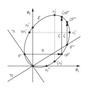
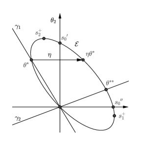
Figure 13. On the left figure : $\eta\theta^{*}$ is the closest pole of $\varphi_{1}$ to $s^{\prime\prime}_{0}$ on $]s^{\prime\prime}_{0},s_{2}^{+}[$, $\zeta\eta\theta^{*}$ is the closest pole of $\varphi_{2}$ to $s^{\prime}_{0}$ on $]s_{1}^{+},s_{0}[$. On the right figure: $\eta\theta^{*}$ is the closest pole of $\varphi_{1}$ to $s^{\prime\prime}_{0}$ on $]s^{\prime\prime}_{0},s_{2}^{+}[$, there are no poles of $\varphi_{2}$ on $]s_{1}^{+},s_{0}[$

We will also need the following two lemmas.

Lemma 14.

• Assume that $\theta_{2}(s_{1}^{+})>0$. Then for any $s\in]\eta s_{1}^{+},s_{0}[$ we have $\theta_{2}(\zeta\eta s)>\theta_{2}(\eta s)$.

• Assume that $\theta_{1}(s_{2}^{+})>0$. Then for any $s\in]s_{0},\zeta s_{2}^{+}[$ we have $\theta_{1}(\eta\zeta s)>\theta_{1}(\zeta s)$.

Proof.

Since $\theta_{2}(s_{1}^{+})>0$, then $\theta_{2}(\zeta\eta s_{0})-\theta_{2}(\eta s_{0})>0$. Consider the function $f(s)=\theta_{2}(\zeta s)-\theta_{2}(s)$ for $s\in[s^{\prime\prime}_{0},s_{1}^{+}]$. It depends continuously on $s$ on this arc. We note that $f(s^{\prime\prime}_{0})=\theta_{2}(\zeta\eta s_{0})-\theta_{2}(\eta s_{0})>0$, $f(s_{1}^{+})=0$. Furthermore, since $s_{1}^{-}\not\in[s^{\prime\prime}_{0},s_{1}^{+}]$, then $f(s)\neq 0$ for all $s\in]s^{\prime\prime}_{0},s^{1,+}]$. Hence $f(s)>0$ for all $s\in]s^{\prime\prime}_{0},s_{1}^{+}]$, from where $\theta_{2}(\zeta\eta s)-\theta_{2}(\eta s)=f(\eta s)>0$ for any $s\in\eta]s^{\prime\prime}_{0},s_{1}^{+}]=[\eta s_{1}^{+},s_{0}[$. The proof in the other case is symmetric.

∎

Lemma 15.

Assume that $\gamma_{2}(s)$ has a zero $\theta^{**}\in]s_{0},s_{1}^{+}[$ and $\gamma_{1}(s)$ has a zero $\theta^{*}\in]s_{2}^{+},s_{0}[$. Then one of the following three assertions holds true :

• The closest pole of $\varphi_{2}(\theta_{1}(s))$ to $s^{\prime}_{0}$ on $]s_{1}^{+},s^{\prime}_{0}[$ is $\zeta\theta^{**}$, the closest pole of $\varphi_{1}(\theta_{2}(s))$ to $s^{\prime\prime}_{0}$ on $]s^{\prime\prime}_{0},s_{2}^{+}[$ is $\eta\theta^{*}$, both of them are of the first order.

• The closest pole of $\varphi_{2}(\theta_{1}(s))$ to $s^{\prime}_{0}$ on $]s_{1}^{+},s^{\prime}_{0}[$ is $\zeta\theta^{**}$, it is of the first order. The closest pole of $\varphi_{1}(\theta_{2}(s))$ to $s^{\prime\prime}_{0}$ on $]s^{\prime\prime}_{0},s_{2}^{+}[$ is $\eta\zeta\theta^{**}$ where $\theta_{1}(\eta\zeta\theta^{**})>\theta_{1}(\zeta\theta^{**})$.

• The closest pole of $\varphi_{2}(\theta_{1}(s))$ to $s^{\prime}_{0}$ on $]s_{1}^{+},s^{\prime}_{0}[$ is $\zeta\eta\theta^{*}$ where $\theta_{2}(\zeta\eta\theta^{*})>\theta_{2}(\eta\theta^{*})$. The closest pole of $\varphi_{1}(\theta_{2}(s))$ to $s^{\prime\prime}_{0}$ on $]s^{\prime\prime}_{0},s_{2}^{+}[$ is $\eta\theta^{*}$, it is of the first order.

The case (ii) is illustrated on Figure 13.

Proof.

By Lemma 12 there exist poles of the function $\varphi_{1}(\theta_{2}(s))$ on $]s^{\prime\prime}_{0},s_{2}^{+}[$. By Lemma 13 under parameters such that $\theta_{1}(s_{2}^{+})\leqslant 0$ or $\theta_{1}(s_{2}^{+})>0$ and $\theta^{**}\not\in]s_{0},\zeta s_{2}^{+}[$, $\eta\theta^{*}$ is the closest pole to $s^{\prime\prime}_{0}$ and it is of the first order. By the same lemma under parameters such that $\theta_{1}(s_{2}^{+})>0$ and $\theta^{**}\in]s_{0},\zeta s_{2}^{+}[$, either $\eta\theta^{*}$ or $\eta\zeta\theta^{**}$ is the closest pole to $s^{\prime}_{0}$. By Lemma 13, if $\gamma_{1}(\zeta\theta^{*})\neq 0$, pole $\eta\theta^{*}$ is of the first order. Condition $\gamma_{1}(\zeta\theta^{*})\neq 0$ is equivalent to $\zeta\theta^{*}\neq\theta^{**}$. This means just that pole $\eta\theta^{*}$ is different from $\eta\zeta\theta^{**}$ which is another candidate for the closest pole to $s^{\prime\prime}_{0}$. By Lemma 14 $\theta_{1}(\eta\zeta\theta^{**})>\theta_{1}(\zeta\theta^{**})$ To summarize, one of two following statements holds true:

• Point $\eta\theta^{*}$ is the closest pole of $\varphi_{1}(\theta_{2}(s))$ to $s^{\prime\prime}_{0}$ on $]s^{\prime\prime}_{0},s_{2}^{+}[$ and it is of the first order;

• The parameters are such that $\theta_{1}(s_{2}^{+})>0$ and $\theta^{**}\in]s_{0},\zeta s_{2}^{+}[$. Point $\eta\zeta\theta^{**}$ is the closest pole of $\varphi_{1}(\theta_{2}(s))$ to $s^{\prime\prime}_{0}$ on $]s^{\prime\prime}_{0},s_{2}^{+}[$ and $\theta_{1}(\eta\zeta\theta^{**})>\theta_{1}(\zeta\theta^{**})$.

By Lemmas 12, 13, 14 and the same considerations, one of the following statements about $\varphi_{2}(\theta_{1})$ holds true:

• Pole $\zeta\theta^{**}$ is the closest pole of $\varphi_{2}(\theta_{1}(s))$ to $s^{\prime}_{0}$ on $]s_{1}^{+},s^{\prime}_{0}[$ and it is of the first order.

• The parameters are such that $\theta_{2}(s_{1}^{+})>0$, $\theta^{*}\in]\eta s_{1}^{+},s_{0}[$, point $\zeta\eta\theta^{*}$ is the closest pole of $\varphi_{2}(\theta_{1}(s))$ to $s^{\prime}_{0}$ on $]s_{1}^{+},s^{\prime}_{0}[$ and $\theta_{2}(\zeta\eta\theta^{*})>\theta_{2}(\eta\theta^{*})$

Let us finally prove that (b1) and (b2) can not hold true simultaneously. Assume that $\theta_{2}(s_{1}^{+})>0$, $\theta^{*}\in]\eta s_{1}^{+},s_{0}[$, $\theta_{1}(s_{2}^{+})>0$, $\theta^{**}\in]s_{0},\zeta s_{2}^{+}[$ and e.g. (b2), that is $\zeta\eta\theta^{*}$ is the closest pole to $s_{0}$. Note that in this case $\zeta\theta^{**}\in]s_{2}^{+},s^{\prime}_{0}[$. Then $\zeta\eta\theta^{*}$ is closer to $s^{\prime}_{0}$ than the pole $\zeta\theta^{**}$ on this segment or coincides with it. Hence $\theta_{1}(\zeta\eta\theta^{*})\leqslant\theta_{1}(\zeta\theta^{**})$ and $\theta_{2}(\zeta\eta\theta^{*})\leqslant\theta_{2}(\zeta\theta^{**})$. By Lemma 14 $\theta_{1}(\eta\theta^{*})=\theta_{1}(\zeta\eta\theta^{*})$ and $\theta_{1}(\zeta\theta^{**})<\theta_{1}(\eta\zeta\theta^{**})$, $\theta_{2}(\eta\theta^{*})<\theta_{2}(\zeta\eta\theta^{*})$ and $\theta_{2}(\zeta\theta^{**})=\theta_{2}(\eta\zeta\theta^{**})$. Then $\theta_{1}(\eta\theta^{*})<\theta_{1}(\eta\zeta\theta^{**})$, $\theta_{2}(\eta\theta^{*})<\theta_{2}(\eta\zeta\theta^{**})$. This means that that $\eta\theta^{*}$ is the closest pole of $\varphi_{1}(\theta_{2}(s))$ to $s^{\prime\prime}_{0}$, $\eta\theta^{*}\neq\eta\zeta\theta^{**}$ , so that (b1) is impossible for $\varphi_{1}(\theta_{2}(s))$, then we have (a1).

In the same way assumption (b1) leads to (a2). Thus (b1), (b2) can not hold true simultaneously, the lemma is proved. ∎

4. Contribution of the saddle-point and of the poles to the asymptotic expansion

4.1. Stationary distribution density as a sum of integrals on ${\bf S}$

By the functional equation (4) and the inversion formula of Laplace transform (we refer to [9] and [3]), the density $\pi(x_{1},x_{2})$ can be represented as a double integral

$$\pi(x_{1},x_{2}) =\frac{1}{(2\pi i)^{2}}\int_{-i\infty}^{i\infty}\int_{-i\infty}^{i\infty}e^{-x_{1}\theta_{1}-x_{2}\theta_{2}}\varphi(\theta_{1},\theta_{2})\mathrm{d}\theta_{1}\mathrm{d}\theta_{2}$$

$$=\frac{-1}{(2\pi i)^{2}}\int_{-i\infty}^{i\infty}\int_{-i\infty}^{i\infty}e^{-x_{1}\theta_{1}-x_{2}\theta_{2}}\frac{\gamma_{1}(\theta)\varphi_{1}(\theta_{2})+\gamma_{2}(\theta)\varphi_{2}(\theta_{1})}{\gamma(\theta)}\mathrm{d}\theta_{1}\mathrm{d}\theta_{2}.$$ (40)

We now reduce it to a sum of single integrals.

Lemma 16.

For any $(x_{1},x_{2})\in{\bf R}^{2}_{+}$

$$\pi(x_{1},x_{2})=I_{1}(x_{1},x_{2})+I_{2}(x_{1},x_{2})$$

where

$$I_{1}(x_{1},x_{2}) =\frac{1}{2\pi i}\int_{-i\infty}^{i\infty}\varphi_{2}(\theta_{1})\gamma_{2}(\theta_{1},\Theta_{2}^{+}(\theta_{1}))e^{-x_{1}\theta_{1}-x_{2}\Theta_{2}^{+}(\theta_{1})}\frac{\mathrm{d}\theta_{1}}{\sqrt{d(\theta_{1})}}$$ (41)

and

$$I_{2}(x_{1},x_{2}) =\frac{1}{2\pi i}\int_{-i\infty}^{i\infty}\varphi_{1}(\theta_{2})\gamma_{1}(\Theta_{1}^{+}(\theta_{2}),\theta_{2})e^{-x_{1}\Theta_{1}^{+}(\theta_{2})-x_{2}\theta_{2}}\frac{\mathrm{d}\theta_{2}}{\sqrt{\tilde{d}(\theta_{2})}}.$$ (42)

Proof.

By inversion formula (40)

$$\pi(x_{1},x_{2}) =\frac{-1}{2\pi i}\int_{-i\infty}^{i\infty}\varphi_{2}(\theta_{1})e^{-x_{1}\theta_{1}}\Big{(}\frac{1}{2\pi i}\int_{-i\infty}^{i\infty}\frac{\gamma_{2}(\theta)}{\gamma(\theta)}e^{-x_{2}\theta_{2}}\mathrm{d}\theta_{2}\Big{)}\mathrm{d}\theta_{1}$$

$$+\frac{-1}{2\pi i}\int_{-i\infty}^{i\infty}\varphi_{1}(\theta_{2})e^{-x_{2}\theta_{2}}\Big{(}\frac{1}{2\pi i}\int_{-i\infty}^{i\infty}\frac{\gamma_{1}(\theta)}{\gamma(\theta)}e^{-x_{1}\theta_{1}}\mathrm{d}\theta_{1}\Big{)}\mathrm{d}\theta_{2}.$$

Now it suffices to show the following formulas

$$\frac{-1}{2\pi i}\int_{-i\infty}^{i\infty}\frac{\gamma_{2}(\theta)e^{-x_{2}\theta_{2}}}{\gamma(\theta)}\mathrm{d}\theta_{2}=\frac{\gamma_{2}(\theta_{1},\Theta_{2}^{+}(\theta_{1}))}{\sqrt{d(\theta_{1})}}e^{-x_{2}\Theta_{2}^{+}(\theta_{1})},$$ (43)

$$\frac{-1}{2\pi i}\int_{-i\infty}^{i\infty}\frac{\gamma_{1}(\theta)e^{-x_{1}\theta_{1}}}{\gamma(\theta)}\mathrm{d}\theta_{1}=\frac{\gamma_{1}(\Theta_{1}^{+}(\theta_{2}),\theta_{2})}{\sqrt{\tilde{d}(\theta_{2})}}e^{-x_{1}\Theta_{1}^{+}(\theta_{2})}.$$ (44)

Let us prove (43). For any $\theta_{1}\in i{\bf R}\setminus\{0\}$, the function $\gamma(\theta)=\frac{\sigma_{22}}{2}(\theta_{2}-\Theta_{2}^{+}(\theta_{1}))(\theta_{2}-\Theta_{2}^{-}(\theta_{1}))$ has two zeros $\Theta_{2}^{+}(\theta_{1})$ and $\Theta_{2}^{-}(\theta_{1})$. Their real parts are of opposite signs: $\Re(\Theta_{2}^{-}(\theta_{1}))<0$ and $\Re(\Theta_{2}^{+}(\theta_{1}))>0$. Thus for any fixed $\theta_{1}\in i{\bf R}\setminus\{0\}$, function $\frac{\gamma_{2}(\theta)e^{-x_{2}\theta_{2}}}{\gamma(\theta)}$ of the argument $\theta_{2}$ has two poles on the complex plane ${\bf C}_{\theta_{2}}$, one at $\Theta^{-}_{2}(\theta_{1})$ with negative real part and another one at $\Theta^{+}_{2}(\theta_{1})$ with positive real part. Let us construct a contour $\mathcal{C}_{R}=[-iR,iR]\cup\{Re^{it}\mid t\in]-\pi/2,\pi/2[\}$ composed of the purely imaginary segment $[-iR,iR]$ and the half of the circle with radius $R$ and center $0$ on ${\bf C}_{\theta_{2}}$, see Figure 14. For $R$ large enough $\Theta^{+}_{2}(\theta_{1})$ is inside the contour. The integral of $\frac{\gamma_{2}(\theta)e^{-x_{2}\theta_{2}}}{\gamma(\theta)}$ over this contour taken in the counter-clockwise direction equals the residue at the unique pole of the integrand:

$$\frac{1}{2\pi i}\int_{\mathcal{C}_{R}}\frac{\gamma_{2}(\theta)e^{-x_{2}\theta_{2}}}{\gamma(\theta)}d\theta_{2}={\rm res}_{\theta_{2}=\Theta^{+}_{2}(\theta_{1})}\frac{\gamma_{2}(\theta)e^{-x_{2}\theta_{2}}}{\gamma(\theta)}=\frac{\gamma_{2}(\theta_{1},\Theta^{+}_{2}(\theta_{1}))}{(\sigma_{22}/2)(\Theta^{+}_{2}(\theta_{1})-\Theta^{-}_{2}(\theta_{1}))}e^{-x_{2}\Theta^{+}_{2}(\theta_{1})}$$

$$=\frac{\gamma_{2}(\theta_{1},\Theta^{+}_{2}(\theta_{1}))}{\sqrt{d(\theta_{1})}}e^{-x_{2}\Theta^{+}_{2}(\theta_{1})}\ \ \ \hbox{ for all large enough }R\geqslant 0.$$ (45)

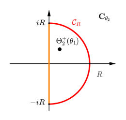
Figure 14. Contour $\mathcal{C}_{R}$ on ${\bf C}_{\theta_{2}}$.

Let us take the limit of this integral as $R\to\infty$:

$$\lim_{R\to\infty}\int_{\mathcal{C}_{R}}\frac{\gamma_{2}(\theta)e^{-x_{2}\theta_{2}}}{\gamma(\theta)}d\theta_{2}=-\lim_{R\to\infty}\int_{-iR}^{iR}\frac{\gamma_{2}(\theta)e^{-x_{2}\theta_{2}}}{\gamma(\theta)}d\theta_{2}+\lim_{R\to\infty}\int_{\{Re^{it}|t\in]-\frac{\pi}{2},\frac{\pi}{2}[\}}\frac{\gamma_{2}(\theta)e^{-x_{2}\theta_{2}}}{\gamma(\theta)}d\theta_{2}.$$ (46)

The last term equals

$$\lim_{R\to\infty}\int_{\{Re^{it}|t\in]-\frac{\pi}{2},\frac{\pi}{2}[\}}\frac{\gamma_{2}(\theta)e^{-x_{2}\theta_{2}}}{\gamma(\theta)}d\theta_{2}=\lim_{R\to\infty}\int_{-\frac{\pi}{2}}^{\frac{\pi}{2}}\frac{\gamma_{2}(\theta_{1},Re^{it})}{\gamma(\theta_{1},Re^{it})}e^{-x_{2}Re^{it}}iRe^{it}dt.$$ (47)

We note that $\sup_{R>0}\sup_{t\in]-\frac{\pi}{2},\frac{\pi}{2}[}|iRe^{it}\frac{\gamma_{2}(\theta_{1},Re^{it})}{\gamma(\theta_{1},Re^{it})}|<\infty$ and $\sup_{R>0}\sup_{t\in]-\frac{\pi}{2},\frac{\pi}{2}[}|e^{-x_{2}Re^{it}}|\leqslant 1$. Furthermore $|e^{-x_{2}Re^{it}}|=e^{-x_{2}R\cos{t}}\to 0$ as $R\to\infty$ for all $t\in]-\frac{\pi}{2},\frac{\pi}{2}[$. Then by dominated convergence theorem the limit (47) equals 0 as $R\to\infty$. Hence, due to (45) and (46)

$$\frac{\gamma_{2}(\theta_{1},\Theta^{+}_{2}(\theta_{1}))}{(\sigma_{22}/2)(\Theta^{+}_{2}(\theta_{1})-\Theta^{-}_{2}(\theta_{1}))}e^{-x_{2}\Theta^{+}_{2}(\theta_{1})}=\lim_{R\to\infty}\int_{\mathcal{C}_{R}}\frac{\gamma_{2}(\theta)e^{-x_{2}\theta_{2}}}{\gamma(\theta)}d\theta_{2}=\int_{-i\infty}^{i\infty}\frac{\gamma_{2}(\theta)e^{-x_{2}\theta_{2}}}{\gamma(\theta)}d\theta_{2},$$

that proves (43) for any $\theta_{1}\in i{\bf R}\setminus\{0\}$. The proof of (44) is analogous.

Note also that the integral

$$\frac{1}{2\pi i}\int_{-i\infty}^{i\infty}\varphi_{2}(\theta_{1})\gamma_{2}(\theta_{1},\Theta_{2}^{+}(\theta_{1}))e^{-x_{1}\theta_{1}-x_{2}\Theta_{2}^{+}(\theta_{1})}\frac{\mathrm{d}\theta_{1}}{\sqrt{d(\theta_{1})}}$$

is absolutely convergent. In fact $\sup_{\theta_{1}\in i{\bf R}}|\varphi_{2}(\theta_{1})|\leqslant\nu_{2}({\bf R}^{2}_{+})$ by definition of $\varphi_{2}$. It is elementary to see that $\sup_{\theta_{1}\in i{\bf R}}|\gamma_{2}(\theta_{1},\Theta^{+}_{2}(\theta_{1}))d^{-1/2}(\theta_{1})|<\infty$. Furthermore, for any $\theta_{1}\in i{\bf R}$, $\Re\Theta_{2}^{+}(\theta_{1})=\sigma_{22}^{-1}(-\mu_{2}+\Re\sqrt{d(\theta_{1})})$, thus for some constant $c>0$ we have $\Re\Theta_{2}^{+}(\theta_{1})>c|\Im\theta_{1}|$. Then the integral is absolutely convergent. This concludes the proof of formula (41). The proof of (42) is completely analogous. ∎

Remark

These integrals are equal to those on the Riemann surface ${\bf S}$ along properly oriented contours ${\cal I}_{\theta_{1}}^{+}$ and ${\cal I}_{\theta_{2}}^{+}$ respectively. Thanks to the parametrization of Section 2.5 we have

$$\frac{\mathrm{d}\theta_{1}}{\sqrt{d(\theta_{1})}}=\frac{\mathrm{d}\theta_{2}}{\sqrt{\tilde{d}(\theta_{2})}}=\frac{i\mathrm{d}s}{s\sqrt{\det\Sigma}}.$$ (48)

Then we can write for $x=(x_{1},x_{2})\in{\bf R}_{+}^{2}$ the density $\pi(x_{1},x_{2})$ as a sum of two integrals on ${\bf S}$ :

$$I_{1}+I_{2}=\frac{1}{2\pi\sqrt{\det\Sigma}}\int_{\mathcal{I}_{\theta_{1}}^{+}}\frac{\varphi_{2}(s)\gamma_{2}(\theta(s))}{s}e^{-\langle\theta(s)\mid x\rangle}{\mathrm{d}s}+\frac{1}{2\pi\sqrt{\det\Sigma}}\int_{\mathcal{I}_{\theta_{2}}^{+}}\frac{\varphi_{1}(s)\gamma_{1}(\theta(s))}{s}e^{-\langle\theta(s)\mid x\rangle}\mathrm{d}s.$$

4.2. Saddle-point

Let us fix $\alpha\in]0,\pi/2[$ and put $(x_{1},x_{2})=re_{\alpha}=r(\cos(\alpha),\sin(\alpha))$ where $\alpha\in]0,\pi/2[$, Our aim now is to find the asymptotic expansion of $\pi(r\cos(\alpha),r\sin(\alpha))$, that is the one of the sum

$$I_{1}+I_{2}=\frac{1}{2\pi\sqrt{\det\Sigma}}\int_{\mathcal{I}_{\theta_{1}}^{+}}\frac{\varphi_{2}(s)\gamma_{2}(\theta(s))}{s}e^{-r\langle\theta(s)\mid e_{\alpha}\rangle}{\mathrm{d}s}+\frac{1}{2\pi\sqrt{\det\Sigma}}\int_{\mathcal{I}_{\theta_{2}}^{+}}\frac{\varphi_{1}(s)\gamma_{1}(\theta(s))}{s}e^{-r\langle\theta(s)\mid e_{\alpha}\rangle}\mathrm{d}s$$ (49)

as $r\to\infty$ and to prove that for any $\alpha_{0}\in]0,\pi/2[$ this asymptotic expansion is uniform in a small neighborhood ${\cal O}(\alpha_{0})\in]0,\pi/2[$.

These integrals are typical to apply the saddle-point method, see [15] or [37]. Let us study the function $\langle\theta(s)\mid e_{\alpha}\rangle$ on ${\bf S}$ and its critical points.

Lemma 17.

• For any $\alpha\in]0,\pi/2[$ function $\langle\theta(s)\mid e_{\alpha}\rangle$ has two critical points on ${\bf S}$ denoted by $\theta^{+}(\alpha)$ and $\theta^{-}(\alpha)$. Both of them are on ellipse $\mathcal{E}$, $\theta^{+}(\alpha)\in]s_{1}^{+},s_{2}^{+}[$, $\theta^{-}(\alpha)\in]s_{1}^{-},s_{2}^{-}[$. Both of them are non-degenerate.

• The coordinates of $\theta^{+}(\alpha)=(\theta_{1}^{+}(\alpha),\theta_{2}^{+}(\alpha))$ are given by formulas :

  $$\theta_{1}^{\pm}(\alpha) = \frac{\mu_{2}\sigma_{12}-\mu_{1}\sigma_{22}}{\det\Sigma}\pm\frac{1}{\det\Sigma}\sqrt{\frac{D_{1}}{1+\frac{\tan(\alpha)^{2}}{(\sigma_{22}-\tan(\alpha)\sigma_{12})^{2}}\det\Sigma}}$$

  $$\theta_{2}^{\pm}(\alpha) = \frac{\mu_{1}\sigma_{12}-\mu_{2}\sigma_{11}}{\det\Sigma}\pm\frac{1}{\det\Sigma}\sqrt{\frac{D_{2}}{1+\frac{\tan(\alpha)^{2}}{(\sigma_{11}-\tan(\alpha)\sigma_{12})^{2}}\det\Sigma}}$$ (50)

  where notations $D_{1}=(\mu_{2}\sigma_{12}-\mu_{1}\sigma_{22})^{2}+\mu_{2}^{2}\det{\Sigma}$ and $D_{2}=(\mu_{1}\sigma_{12}-\mu_{2}\sigma_{11})^{2}+\mu_{1}^{2}\det{\Sigma}$ are used. With the parametrization of Section 2.5 the corresponding points on $\bf S$ are such that:

  $$s_{\pm}(\alpha)^{2}=\frac{\cos\alpha(\theta_{1}^{+}-\theta_{1}^{-})+\sin\alpha(\theta_{2}^{+}-\theta_{2}^{-})e^{i\beta}}{\cos\alpha(\theta_{1}^{+}-\theta_{1}^{-})+\sin\alpha(\theta_{2}^{+}-\theta_{2}^{-})e^{-i\beta}}.$$

• Function $\theta^{+}(\alpha)$ is an isomorphism between $[0,\pi/2]$ and ${\cal A}=[s^{1,+},s^{2,+}]$, $\lim_{\alpha\to 0}\theta^{+}(\alpha)=s_{1}^{+}$, $\lim_{\alpha\to\pi/2}\theta^{+}(\alpha)=s_{2}^{+}$. Function $\theta^{-}(\alpha)$ is an isomorphism between $[0,\pi/2]$ and $[s^{1,-},s^{2,-}]$, $\lim_{\alpha\to 0}\theta^{-}(\alpha)=s_{1}^{-}$, $\lim_{\alpha\to\pi/2}\theta^{-}(\alpha)=s_{2}^{-}$.

• Function $\langle\theta(s)\mid e_{\alpha}\rangle$ is strictly increasing on the arc $[\theta^{-}(\alpha),\theta^{+}(\alpha)]$ of $\mathcal{E}$ and strictly decreasing on the arc $[\theta^{+}(\alpha),\theta^{-}(\alpha)]$. Namely, $\theta^{+}(\alpha)$ is its maximum on $\cal{E}$ and $\theta^{-}(\alpha)$ is its minimum:

  $$\theta^{+}(\alpha)={\rm argmax}_{s\in{\cal E}}\langle\theta(s)\mid e_{\alpha}\rangle\ \ \ \theta^{-}(\alpha)={\rm argmin}_{s\in{\cal E}}\langle\theta(s)\mid e_{\alpha}\rangle.$$

Proof.

Let us look for critical points with coordinates $(\theta_{1},\theta_{2})$ of $\langle\theta(s)\mid e_{\alpha}\rangle$ on ${\bf S}$. Equation $(\theta_{1}\cos(\alpha)+\theta_{2}(\theta_{1})\sin(\alpha))^{\prime}_{\theta_{1}}=0$ implies $\tan(\alpha)\frac{d\theta_{2}}{d\theta_{1}}=-1$. Substituting it into equation $\gamma(\theta_{1},\theta_{2}(\theta_{1}))^{\prime}_{\theta_{1}}\equiv 0$ and writing also $\gamma(\theta_{1},\theta_{2})\equiv 0$ we get the system of two equations

$$\left\{\begin{array}[]{l}-\sigma_{11}\theta_{1}\tan(\alpha)+\sigma_{22}\theta_{2}+\sigma_{12}\theta_{1}-\sigma_{12}\theta_{2}\tan(\alpha)-\mu_{1}\tan(\alpha)+\mu_{2}=0\\ \sigma_{11}\theta_{1}^{2}+\sigma_{22}\theta_{2}^{2}+2\sigma_{12}\theta_{1}\theta_{2}+\mu_{1}\theta_{1}+\mu_{2}\theta_{2}=0\end{array}\right.$$

from where we compute $\theta^{-}(\alpha)=(\theta^{-}_{1}(\alpha),\theta^{-}_{2}(\alpha))$ and $\theta^{+}(\alpha)=(\theta^{+}_{1}(\alpha),\theta^{+}_{2}(\alpha))$ explicitly as announced in (50). We check directly that $\frac{d^{2}\theta_{2}}{d\theta_{1}}\neq 0$ at these points, so they are non-degenerate critical points. It is also easy to see from (50) that $\theta^{-}_{1}(\alpha)$ is strictly increasing from branch point $\theta_{1}^{-}$ to $\theta_{1}(\theta_{2}^{-})$ and that $\theta^{+}_{1}(\alpha)$ is strictly decreasing from branch point $\theta_{1}^{+}$ to $\theta_{1}(\theta_{2}^{+})$ when $\alpha$ runs the segment $[0,\pi/2]$. In the same way $\theta^{-}_{2}(\alpha)$ is strictly decreasing from $\theta_{2}(\theta_{1}^{-})$ to $\theta_{2}^{-}$ and $\theta^{+}_{2}(\alpha)$ is strictly increasing from $\theta_{2}(\theta_{1}^{+})$ to $\theta_{2}^{+}$ when $\alpha$ runs the segment $[0,\pi/2]$. This proves assertions (i)–(iii).

Finally, since there are no critical points on $\cal{E}$ except for $\theta^{+}(\alpha)$ and $\theta^{-}(\alpha)$, function $\langle\theta(s)\mid e_{\alpha}\rangle$ is monotonous on the arcs $[\theta^{-}(\alpha),\theta^{+}(\alpha)]$ and $[\theta^{+}(\alpha),\theta^{-}(\alpha)]$. In view of the inequality $\langle\theta^{+}(\alpha)\mid e_{\alpha}\rangle>\langle\theta^{-}(\alpha)\mid e_{\alpha}\rangle$, assertion (iv) follows. ∎

Notation of the saddle-point. From now one we are interested in point $\theta^{+}(\alpha)$ that we denote by $\theta(\alpha)$ for shortness.

The steepest-descent contour $\gamma_{\alpha}$. The level curves $\{s:\Re\langle\theta(s)\mid e_{\alpha}\rangle=\langle\theta(\alpha)\mid e_{\alpha}\rangle\}$ are orthogonal at $\theta(\alpha)$ and subdivide its neighborhood into four sections. The curves of steepest descent $\{s:\Im\langle\theta(s)\mid e_{\alpha}\rangle=0\}$ on ${\bf S}$ are orthogonal at $\theta(\alpha)$ as well, see Lemma 1.3, Chapter IV in [14]. One of them coincides with $\cal{E}$. We denote the other one by $\gamma_{\alpha}$. The real part $\Re\langle\theta(s)\mid\alpha\rangle$ is strictly increasing on $\gamma_{\alpha}$ as $s$ goes far away from $\theta(\alpha)$, see [15, Section 4.2]. The level curves of functions $\Re\langle\theta(s)\mid e_{\alpha}\rangle$ and $\Im\langle\theta(s)\mid e_{\alpha}\rangle$ are pictured in Figure 15.

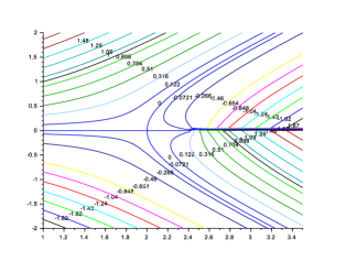
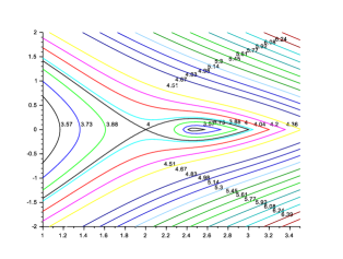
Figure 15. Level sets of $\Im\langle\theta(s)\mid e_{\alpha}\rangle$ and $\Re\langle\theta(s)\mid e_{\alpha}\rangle$

Let $z_{\alpha,+}=(\theta_{1}(z_{\alpha,+}),\theta_{2}(z_{\alpha,+}))$ and $z_{\alpha,-}=(\theta_{1}(z_{\alpha,-}),\theta_{2}(z_{\alpha,-}))$ be the end points of $\gamma_{\alpha}$ where $\Im\theta_{1}(z_{\alpha,-})>0$ and $\Im\theta_{1}(z_{\alpha,-})<0$. We can fix end points $z_{\alpha,-}$ and $z_{\alpha,+}$ in such a way that $\forall\alpha\in\mathcal{O}(\alpha_{0})$ and some small $\epsilon>0$

$$\Re\langle z_{\alpha,\pm}\mid e_{\alpha}\rangle=\langle\theta(\alpha)\mid e_{\alpha}\rangle+\epsilon.$$

For technical reasons we choose $\epsilon$ small enough such that $\Re\theta_{1}(z_{\alpha,\pm})\in]\theta_{1}^{-},\theta_{1}^{+}[$ and $\Re\theta_{2}(z_{\alpha,\pm})\in]\theta_{2}^{-},\theta_{2}^{+}[$.

4.3. Shifting the integration contours

Our aim now is to shift the integration contours $\mathcal{I}_{\theta_{1}}^{+}$ and $\mathcal{I}_{\theta_{2}}^{+}$ in (49) up to new contours $\Gamma_{\theta_{1},\alpha}$ and $\Gamma_{\theta_{2},\alpha}$ respectively which coincide with $\gamma_{\alpha}$ in a neighborhood of $\theta(\alpha)$ on ${\bf S}$ and are “higher” than $\theta(\alpha)$ in the sense of level curves of the function $\Re\langle\theta(s)\mid e_{\alpha}\rangle$, that is $\Re\langle\theta(s)\mid e_{\alpha}\rangle>\Re\langle\theta(\alpha)\mid e_{\alpha}\rangle+\epsilon$ for any $s\in\Gamma_{\theta_{i},\alpha}\setminus\gamma_{\alpha}$ with $i=1,2$. When shifting the contours we should of course take into account the poles of the integrands and the residues at them.

Let us construct $\Gamma_{\theta_{1},\alpha}$ and $\Gamma_{\theta_{2},\alpha}$. We set

$$\Gamma_{\theta_{1},\alpha}^{1,+}=\{s:\Re\theta_{1}(s)=\Re\theta_{1}(z_{\alpha,+}),\Im\theta_{1}(z_{\alpha,+})\leqslant\Im\theta_{1}(s)\leqslant V(\alpha)\}$$

where $V(\alpha)>0$ will be defined later. Then the end points of $\Gamma_{\theta_{1},\alpha}^{1,+}$ are $z_{\alpha,+}$ and $Z_{\alpha,+}$ where $\Re\theta_{1}(z_{\alpha,+})=\Re\theta_{1}(Z_{\alpha,+})$, $\Im\theta_{1}(Z_{\alpha,+})=V(\alpha)$. Next

$$\Gamma_{\theta_{1},\alpha}^{2,+}=\{s:\Im\theta_{1}(s)=V(\alpha),0\leqslant\Re\theta_{1}(s)\leqslant\Re\theta_{1}(z_{\alpha,+})\}$$

if $\Re\theta_{1}(z_{\alpha,+})>0$ and

$$\Gamma_{\theta_{1},\alpha}^{2,+}=\{s:\Im\theta_{1}(s)=V(\alpha),0\geqslant\Re\theta_{1}(s)\geqslant\Re\theta_{1}(z_{\alpha,+})\}$$

if $\Re\theta_{1}(z_{\alpha,+})<0$. This contour goes from $Z_{\alpha,+}$ up to $Z^{0}_{\alpha,+}$ on ${\mathcal{I}}_{\theta_{1}}$ with $\Re(\theta_{1}(s))=0$, $\Im(\theta_{1}(s))=V(\alpha)$. Finally $\Gamma_{\theta_{1},\alpha}^{3,+}$ coincides with $\mathcal{I}_{\theta_{1}}^{+}$ from $Z_{\alpha,+}^{0}$ up to infinity :

$$\Gamma_{\theta_{1},\alpha}^{3,+}=\{s:\Re\theta_{1}(s)=0,\Im\theta_{1}(s)\geqslant V(\alpha)\}.$$

We define in the same way $\Gamma_{\theta_{1},\alpha}^{1,-}=\{s:\Re\theta_{1}(s)=\Re\theta_{1}(z_{\alpha,-}),-V(\alpha)\leqslant\Im s\leqslant\Im\theta_{1}(z_{\alpha,-})\}$. The end points of $\Gamma_{\theta_{1},\alpha}^{1,-}$ are $z_{\alpha,-}$ and $Z_{\alpha,-}$ where $\Re\theta_{1}(z_{\alpha,-})=\Re\theta_{1}(Z_{\alpha,-})$, $\Im\theta_{1}(Z_{\alpha,-})=-V(\alpha)$. Next $\Gamma_{\theta_{2},\alpha}^{2,-}=\{s:\Im\theta_{1}(s)=-V(\alpha),0\leqslant\Re\theta_{1}(s)\leqslant\Re\theta_{1}(z_{\alpha,-})\}$ or $\Gamma_{\theta_{2},\alpha}^{2-}=\{s:\Im\theta_{1}(s)=-V(\alpha),0\geqslant\Re\theta_{1}(s)\geqslant\Re\theta_{1}(z_{\alpha,-})\}$ according to the sign of $\Re\theta_{1}(z_{\alpha,-})$. It goes from $Z_{\alpha,-}$ to $Z^{0}_{\alpha,-}$ on ${\bf S}_{\theta_{1}}$ with $\Re(\theta_{1}(Z^{0}_{\alpha,-}))=0$, $\Im(\theta_{1}(Z^{0}_{\alpha,-}))=-V(\alpha)$. Finally $\Gamma_{\theta_{1},\alpha}^{3,+}$ coincides with ${\mathcal{I}}_{\theta_{1}}^{+}$ from $Z_{\alpha,-}^{0}$ up to infinity. Then contour $\Gamma_{\theta_{1},\alpha}=\Gamma_{\theta_{1},\alpha}^{3,-}\cup\Gamma_{\theta_{1},\alpha}^{2,-}\cup\Gamma_{\theta_{1},\alpha}^{1,-}\cup\gamma_{\alpha}\cup\Gamma_{\theta_{1},\alpha}^{1,+}\cup\Gamma_{\theta_{1},\alpha}^{2,+}\cup\Gamma_{\theta_{1},\alpha}^{3,+}\subset{\bf S}_{\theta_{1}}^{1}$. One can visualize this contour on Figure 16 : in the left picture it is drawn on parametrized ${\bf S}$, in the right picture it is projected on the complex plane ${\bf C}_{\theta_{1}}$ .

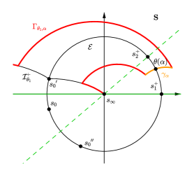
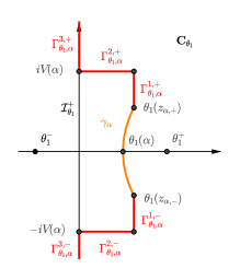
Figure 16. Contour $\Gamma_{\theta_{1},\alpha}$ on parametrized ${\bf S}$ and projected on ${\bf C}_{\theta_{1}}$.

The contour $\Gamma_{\theta_{2},\alpha}$ is constructed analogously with respect to $\theta_{2}$-coordinate, $\Gamma_{\theta_{2},\alpha}=\Gamma_{\theta_{2},\alpha}^{3,-}\cup\Gamma_{\theta_{2},\alpha}^{2,-}\cup\Gamma_{\theta_{2},\alpha}^{1,-}\cup\gamma_{\alpha}\cup\Gamma_{\theta_{2},\alpha}^{1,+}\cup\Gamma_{\theta_{2},\alpha}^{2,+}\cup\Gamma_{\theta_{2},\alpha}^{3,+}\subset{\bf S}_{\theta_{2}}^{1}$. The curve of steepest descent $\gamma_{\alpha}$ is common for $\Gamma_{\theta_{1},\alpha}$ and $\Gamma_{\theta_{2},\alpha}$.

Let us recall that poles of $\varphi_{1}(s)$ and $\varphi_{2}(s)$ on ${\bf S}$ may occur only at $\cal{E}$. Let us also recall the convention that an arc $\}a,b\{$ on $\cal{E}$ is the one with ends $a$ and $b$ which does not include $s_{0}=(0,0)$.

Notation of the sets of poles $\mathcal{P}^{\prime}_{\alpha}$ and $\mathcal{P}^{\prime\prime}_{\alpha}$. Let ${\cal P^{\prime}}_{\alpha}$ be the set of poles of the first order of the function $\varphi_{2}(\theta_{1}(s))$ on the arc $\}\theta(\alpha),s^{\prime}_{0}\{$. Let ${\cal P^{\prime\prime}}_{\alpha}$ be the set of poles of the first order of the function $\varphi_{1}(\theta_{2}(s))$ on the arc $\}\theta(\alpha),s^{\prime\prime}_{0}\{$.

Then the following lemma holds true.

Lemma 18.

Let $\alpha_{0}\in]0,\pi/2[$ be such that $\theta(\alpha_{0})$ is not a pole of $\varphi_{1}(\theta_{2}(s))$ neither of $\varphi_{2}(\theta_{1}(s))$. If ${\cal P^{\prime}}_{\alpha}\cup{\cal P^{\prime\prime}}_{\alpha}$ is not empty, then for any $\alpha\in\mathcal{O}(\alpha_{0})$

$$\pi(re_{\alpha})=\sum_{p\in{\cal P^{\prime}}_{\alpha}}{\rm res}_{p}\varphi_{2}(\theta_{1}(s))\frac{\gamma_{2}(p)}{\sqrt{d(\theta_{1}(p))}}e^{-r\langle\theta(p)\mid e_{\alpha}\rangle}+\sum_{p\in{\cal P^{\prime\prime}}_{\alpha}}{\rm res}_{p}\varphi_{1}(\theta_{2}(s))\frac{\gamma_{1}(p)}{\sqrt{\tilde{d}(\theta_{2}(p))}}e^{-r\langle\theta(p)\mid e_{\alpha}\rangle}$$ (51)

$${}+\frac{1}{2\pi\sqrt{\det\Sigma}}\big{(}\int_{\Gamma_{\theta_{1},\alpha}}\frac{\varphi_{2}(s)\gamma_{2}(\theta(s))}{s}e^{-r\langle\theta(s)\mid e_{\alpha}\rangle}{\mathrm{d}s}+\int_{\Gamma_{\theta_{2},\alpha}}\frac{\varphi_{1}(s)\gamma_{1}(\theta(s))}{s}e^{-r\langle\theta(s)\mid e_{\alpha}\rangle}\big{)}\mathrm{d}s.$$

If $\mathcal{P^{\prime}}_{\alpha}\cup\mathcal{P^{\prime\prime}}_{\alpha}$ is empty, representation (51) stays valid where the corresponding sums over $p\in{\cal P^{\prime}}_{\alpha}$ and $p\in{\cal P^{\prime\prime}}_{\alpha}$ are omitted.

Proof.

It follows from the assumption of the lemma that $\theta(\alpha)$ is not a pole of $\varphi_{1}(\theta_{2}(s))$ neither of $\varphi_{2}(\theta_{1}(s))$ for any $\alpha$ in a small enough neighborhood $\mathcal{O}(\alpha_{0})$. Then we use the representation of the density (49) and apply Cauchy theorem shifting the contours to $\Gamma_{\theta_{1},\alpha}$ and $\Gamma_{\theta_{2},\alpha}$. ∎

In order to find the asymptotic expansion of the density $\pi(r\cos(\alpha),r\sin(\alpha))$, we have to evaluate now the contribution of the residues at poles in (51) and the one of integrals along shifted contours $\Gamma_{\theta_{1},\alpha}$ and $\Gamma_{\theta_{2},\alpha}$. This is the subject of the next two sections.

4.4. Asymptotics of integrals along shifted contours $\Gamma_{\theta_{1},\alpha}$ and $\Gamma_{\theta_{2},\alpha}$

To finish the construction of $\Gamma_{\theta_{1},\alpha}$ and $\Gamma_{\theta_{2},\alpha}$, it remains to specify $V(\alpha)$. For that purpose we consider closer the function

$$f_{\alpha}(s)=\langle\theta(s)\mid e_{\alpha}\rangle=\theta_{1}(s)\cos\alpha+\theta_{2}(s)\sin\alpha.$$

Let us define the projection of this function on ${\bf C}_{\theta_{1}}$ :

$$f_{\alpha}(\theta_{1})=\theta_{1}\cos\alpha+\Theta_{2}^{+}(\theta_{1})\sin\alpha,\ \ \theta_{1}\in{\bf C}_{\theta_{1}}.$$

Clearly $f_{\alpha}(s)=f_{\alpha}(\theta_{1}(s))=\langle\theta(s)\mid e_{\alpha}\rangle$ on ${\bf S}_{\theta_{1}}^{1}$.

Lemma 19.

• For any fixed $u\in[\theta_{1}^{-},\theta_{1}^{+}]$ the function $v\to\Re(f_{\alpha}(u+iv))$ is increasing on $[0,\infty[$ and decreasing on $]-\infty,0]$.

• There exist constants $d_{1}\leqslant 0$, $d_{2}>0$ and $V>0$ such that:

  $$\inf_{u\in[\theta_{1}^{-},\theta_{1}^{+}]}\Re(f_{\alpha}(u+iv))\geqslant d_{1}+d_{2}\sin(\alpha)|v|\ \ \forall v\geqslant V\ \hbox{and }\forall v\leqslant-V,\ \ \forall\alpha\in]0,\pi/2[.$$ (52)

Proof.

We compute :

$$\Re(f_{\alpha}(u+iv))=\cos(\alpha)u+\frac{\sin(\alpha)}{\sigma_{22}}(-\sigma_{12}u-\mu_{2}+\Re\sqrt{d(u+iv)})$$

with the discriminant $d(u+iv)=(\det\Sigma)(u+iv-\theta_{1}^{-})(\theta_{1}^{+}-u-iv)$. Then

$$\Re\sqrt{d(u+iv)}=\sqrt{\det\Sigma}\sqrt{|(u+iv-\theta_{1}^{-})(\theta_{1}^{+}-u-iv)|}\cos(\frac{\omega_{-}(u+iv)+\omega_{+}(u+iv)}{2})$$

where $\omega_{-}(u+iv)$ et $\omega_{+}(u+iv)$ are defined as $\omega_{-}(u+iv)=\arg(\theta_{1}^{+}-u-iv)$ and $\omega_{+}(u+iv)=\arg(u+iv-\theta_{1}^{-})$, see Figure 17. We have

$$\cos(\frac{\omega_{-}(u+iv)+\omega_{+}(u+iv)}{2})=\sqrt{\frac{1}{2}\cos(\omega_{-}(u+iv)+\omega_{+}(u+iv))+\frac{1}{2}}$$

$$=\sqrt{\frac{1}{2}\cos(\omega_{-}(u+iv))\cos(\omega_{+}(u+iv))-\frac{1}{2}\sin(\omega_{-}(u+iv))\sin(\omega_{+}(u+iv))+\frac{1}{2}}$$

$$=\sqrt{\frac{(u-\theta_{1}^{-})(\theta_{1}^{+}-u)-v(-v)}{2|(u+iv-\theta_{1}^{-})(\theta_{1}^{+}-u-iv)|}+\frac{1}{2}}.$$

Thus

$$\Re(f_{\alpha}(u+iv))=\cos(\alpha)u\\ +\frac{\sin(\alpha)}{\sigma_{22}}\Big{(}-\sigma_{12}u-\mu_{2}+\sqrt{\frac{1}{2}}\sqrt{(u-\theta_{1}^{-})(\theta_{1}^{+}-u)+v^{2}+|(u+iv-\theta_{1}^{-})(\theta_{1}^{+}-u-iv)|}\Big{)}$$

Both statements of the lemma follow directly from this representation. ∎

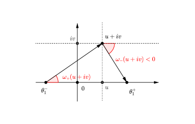
Figure 17. $\omega_{-}(u+iv)$ et $\omega_{+}(u+iv)$

We may now choose $V(\alpha)$ and such that

$$V(\alpha)=\max\Big{(}V,\ \frac{\langle\theta(\alpha)\mid e_{\alpha}\rangle+\epsilon-d_{1}}{d_{2}\sin(\alpha)}\Big{)}$$ (53)

in accordance with notations of Lemma 19. This concludes the construction of $\Gamma_{\theta_{1},\alpha}$ and $\Gamma_{\theta_{2},\alpha}$.

The asymptotic expansion of integrals along these contours is given in the following lemma. The main contribution comes from the integrals along $\gamma_{\alpha}$, while all other parts of integrals are proved to be exponentially negligible by construction.

Lemma 20.

Let $\alpha_{0}\in]0,\pi/2[$ and $\mathcal{O}(\alpha_{0})$ a small enough neighborhood of $\alpha_{0}$. Then when $r\to\infty$ uniformly for $\alpha\in\mathcal{O}(\alpha_{0})$ we have

$$\frac{1}{2\pi\sqrt{\det\Sigma}}\int_{\Gamma_{\theta_{1},\alpha}}\frac{\varphi_{2}(s)\gamma_{2}(\theta(s))}{s}e^{-r\langle\theta(s)\mid e_{\alpha}\rangle}{\mathrm{d}s}\sim\sum_{l=0}^{k}\frac{c^{l}_{\theta_{1}}(\alpha)}{r^{l}\sqrt{r}}e^{-r\langle\theta(\alpha)\mid e_{\alpha}\rangle},$$ (54)

$$\frac{1}{2\pi\sqrt{\det\Sigma}}\int_{\Gamma_{\theta_{2},\alpha}}\frac{\varphi_{1}(s)\gamma_{1}(\theta(s))}{s}e^{-r\langle\theta(s)\mid e_{\alpha}\rangle}\mathrm{d}s\sim\sum_{l=0}^{k}\frac{c^{l}_{\theta_{2}}(\alpha)}{r^{l}\sqrt{r}}e^{-r\langle\theta(\alpha)\mid e_{\alpha}\rangle}.$$ (55)

The constants $c^{l}_{\theta_{1}}(\alpha)$, $c^{l}_{\theta_{2}}(\alpha)$, $l=0,1,2,\ldots$ depend continuously of $\alpha$ and can be made explicit in terms of functions $\varphi_{1}$ and $\varphi_{2}$ and their derivatives at $\theta(\alpha)$. Namely

$$c^{0}_{\theta_{1}}(\alpha) = \frac{1}{\sqrt{2\pi\det\Sigma}}\frac{\varphi_{2}(s(\alpha))\gamma_{2}(\theta(\alpha))}{s(\alpha)\sqrt{f_{\alpha}^{\prime\prime}(s(\alpha))}},$$

$$c^{0}_{\theta_{2}}(\alpha) = \frac{1}{\sqrt{2\pi\det\Sigma}}\frac{\varphi_{1}(s(\alpha))\gamma_{1}(\theta(\alpha))}{s(\alpha)\sqrt{f_{\alpha}^{\prime\prime}(s(\alpha))}}.$$

Proof.

By Lemma 19 (i) and by (48) for any $r>0$.

$$\Big{|}\int_{\Gamma_{\theta_{1},\alpha}^{1,\pm}}\frac{\varphi_{2}(\theta_{1}(s))\gamma_{2}(s)}{s\sqrt{\det\Sigma}}\exp^{-r\langle\theta(s)\mid e_{\alpha}\rangle}{\rm d}\,s\Big{|}\leqslant 2V(\alpha)\sup_{s\in\Gamma_{\theta_{1},\alpha}^{1,\pm}}\Big{|}\frac{\varphi_{2}(\theta_{1}(s))\gamma_{2}(s)}{\sqrt{d(\theta_{1}(s))}}\Big{|}e^{-r\langle\theta(\alpha)\mid e_{\alpha}\rangle-r\epsilon}.$$ (56)

The length of $\Gamma_{\theta_{2},\alpha}^{\pm}$ being smaller than $(\theta_{1}^{+}-\theta_{1}^{-})$, by Lemma 19 (ii) and by (48) for any $r>0$

$$\Big{|}\int_{\Gamma_{\theta_{1},\alpha}^{2,\pm}}\frac{\varphi_{2}(\theta_{1}(s))\gamma_{2}(s)}{s\sqrt{\det\Sigma}}\exp^{-r\langle\theta(s)\mid e_{\alpha}\rangle}{\rm d}\,s\Big{|}\leqslant(\theta_{1}^{+}-\theta_{1}^{-})\sup_{s\in\Gamma_{\theta_{2},\alpha}^{2,\pm}}\Big{|}\frac{\varphi_{2}(\theta_{1}(s))\gamma_{2}(s)}{\sqrt{d(\theta_{1}(s))}}\Big{|}e^{-r(d_{1}+d_{2}\sin(\alpha)V(\alpha))}$$ (57)

where due to the choice (53) of $V(\alpha)$

$$e^{-r(d_{1}+d_{2}\sin(\alpha)V(\alpha))}\leqslant e^{-r\langle\theta(\alpha)\mid e_{\alpha}\rangle-r\epsilon}.$$ (58)

Finally note that for any $s\in\Gamma_{\theta_{1},\alpha}^{3,\pm}$

$$\frac{\gamma_{2}(s)}{\sqrt{d(\theta_{1}(s))}}=r_{1,2}\frac{\theta_{1}(s)}{\sqrt{d(\theta_{1}(s))}}+r_{22}\frac{-b(\theta_{1}(s))+\sqrt{d(\theta_{1}(s))}}{2a(\theta_{1}(s))\sqrt{d(\theta_{1}(s))}}$$

where $\Re\theta_{1}(s)=0$, $\Im\theta_{1}(s)\geqslant V$. Then there exists a constant $D>0$ such that $|\gamma_{2}(s)d^{-1/2}(\theta_{1}(s))|\leqslant D$ for any $s\in\Gamma_{\theta_{1},\alpha}^{3,\pm}$ and any $\alpha\in]0,\pi/2[$. Moreover $|\varphi_{2}(\theta_{1}(s))|\leqslant\nu_{1}({\bf R_{+}})$ for any $s\in{\mathcal{I}}_{\theta_{1}}$. Thus by Lemma 19 (ii) and by (48)

$$\Big{|}\int_{\Gamma_{\theta_{1},\alpha}^{3,\pm}}\frac{\varphi_{2}(\theta_{1}(s))\gamma_{2}(s)}{s\sqrt{\det\Sigma}}\exp^{-r\langle\theta(s)\mid e_{\alpha}\rangle}{\rm d}\,s\Big{|}\leqslant 2D\nu_{1}({\bf R_{+}})\int\limits_{V(\alpha)}^{\infty}e^{-r(d_{1}+d_{2}\sin(\alpha)v)}dv$$

$$\leqslant 2D\nu_{1}({\bf R_{+}})\frac{1}{c\sin(\alpha)V(\alpha)}e^{-r(d_{1}+d_{2}\sin(\alpha)V(\alpha))}\leqslant 2D\nu_{1}({\bf R_{+}})\frac{1}{c\sin(\alpha)V(\alpha)}e^{-r\langle\theta(\alpha)\mid e_{\alpha}\rangle-r\epsilon}.$$ (59)

The contours $\Gamma_{\theta_{1},\alpha}^{i,\pm}$ for $i=1,2$ being far away from poles of $\varphi_{2}$ and zeros of $d(\theta_{1}(s))$ for all $\alpha\in{\cal O}(\alpha_{0})$, $\sup_{\alpha\in{\cal O}(\alpha_{0})}\sup_{s\in\Gamma_{\theta_{1},\alpha}^{i,\pm}}\Big{|}\frac{\varphi_{2}(\theta_{1}(s))\gamma_{2}(s)}{\sqrt{d(\theta_{1}(s))}}\Big{|}<\infty$ for $i=1,2$, and of course $\sup_{\alpha\in{\cal O}(\alpha_{0})}(\sin(\alpha)V(\alpha))^{-1}$ and $\sup_{\alpha\in{\cal O}(\alpha_{0})}V(\alpha)$ are finite as well. It follows that for some constant $C>0$ , any $r>0$ and any $\alpha\in{\cal O}(\alpha_{0})$

$$\Big{|}\int_{\Gamma_{\theta_{1},\alpha}^{1,\pm}\cup\Gamma_{\theta_{1},\alpha}^{2,\pm}\cup\Gamma_{\theta_{1},\alpha}^{3,\pm}}\frac{\varphi_{2}(\theta_{1}(s))\gamma_{2}(s)}{s\sqrt{\det\Sigma}}e^{-r\langle\theta(s)\mid e_{\alpha}\rangle}{\rm d}\,s\Big{|}\leqslant Ce^{-r\langle\theta(\alpha)\mid e_{\alpha}\rangle-r\epsilon}.$$ (60)

As for the contour $\gamma_{\alpha}$ of the steepest descent of the function $\langle\theta(s)\mid e_{\alpha}\rangle$, we apply the standard saddle-point method, see e.g. Theorem 1.7, Chapter IV in [14]: for any $k>0$ when $r\to\infty$, uniformly $\forall\alpha\in{\mathcal{O}}(\alpha_{0})$,

$$\frac{1}{2\pi\sqrt{\det\Sigma}}\int_{\gamma_{\alpha}}\frac{\varphi_{2}(s)\gamma_{2}(\theta(s))}{s}e^{-r\langle\theta(s)\mid e_{\alpha}\rangle}{\rm d}\,s\sim\sum_{l=0}^{k}\frac{c^{l}_{\theta_{1}}(\alpha)}{r^{l}\sqrt{r}}e^{-r\langle\theta(\alpha)\mid e_{\alpha}\rangle},$$ (61)

where $c^{0}_{\theta_{1}}(\alpha)$ is given explicitly in the statement of the lemma and all other constants $c^{l}_{\theta_{1}}(\alpha)$ can be written in terms of the same functions and their derivatives at $\theta(\alpha)$. Thus (54) is proved and the proof of (55) for the integral over $\Gamma_{\theta_{2},\alpha}$ is absolutely analogous. ∎

4.5. Contribution of poles into the asymptotics of $\pi(r\cos(\alpha),r\sin(\alpha))$

Once Lemma 20 established the asymptotics of integrals along shifted contours $\Gamma_{\theta_{1},\alpha}$ and $\Gamma_{\theta_{2},\alpha}$, let us come back to Lemma 18 and evaluate the contribution to the density of residues at poles over $\mathcal{P}^{\prime}_{\alpha}\cup\mathcal{P}^{\prime\prime}_{\alpha}$. There are two possibilities:

• $\mathcal{P}^{\prime}_{\alpha}\cup\mathcal{P}^{\prime\prime}_{\alpha}$ is empty, then the asymptotics of the density is determined by the saddle-point via Lemma 20.

• $\mathcal{P}^{\prime}_{\alpha}\cup\mathcal{P}^{\prime\prime}_{\alpha}$ is not empty. Then due to monotonicity of the function $\langle\theta(s)\mid e_{\alpha}\rangle$ on $\mathcal{E}$, see Lemma 17 (iv), for any $p\in\mathcal{P}^{\prime}_{\alpha}\cup\mathcal{P}^{\prime\prime}_{\alpha}$ we have $\langle\theta(p)\mid e_{\alpha}\rangle<\langle\theta(\alpha)\mid e_{\alpha}\rangle$. Hence all residues at poles $p\in\mathcal{P}^{\prime}_{\alpha}\cup\mathcal{P}^{\prime\prime}_{\alpha}$ bring more important contribution to the asymptotic expansion as $r\to\infty$ than integrals over $\Gamma_{\theta_{1},\alpha}$ and $\Gamma_{\theta_{2},\alpha}$.

First of all, we would like to distinguish the set of parameters $(\Sigma,\mu,R)$ under which (i) or (ii) hold true. Secondly, under (ii), we would like to find the most important pole from the asymptotic point of view. Let us look closer at the arc $\{s^{\prime}_{0},\theta(\alpha)\}$. Under parameters such that $\theta_{1}(s_{2}^{+})<0$ we have $s^{\prime}_{0}\in]s_{1}^{+},s_{2}^{+}[$, see Figure 18, the left picture. Then for some $\alpha^{\prime}\in]0,\pi/2[$ $\theta(\alpha^{\prime})=s^{\prime}_{0}$. This arc written in square brackets in the anticlockwise direction is $]s^{\prime}_{0},\theta(\alpha)[$ for any $\alpha\in]\alpha^{\prime},\pi/2[$ and the function $\langle\theta(s)\mid e_{\alpha}\rangle$ is increasing when $s$ runs from $s^{\prime}_{0}$ to $\theta(\alpha)$. For any $\alpha\in[0,\alpha^{\prime}[$ this arc is written $]\theta(\alpha),s^{\prime}_{0}[$ and the function $\langle\theta(s)\mid e_{\alpha}\rangle$ is decreasing when $s$ runs from $\theta(\alpha)$ so $s^{\prime}_{0}$. Under parameters such that $\theta_{1}(s_{2}^{+})\geqslant 0$, we have $s^{\prime}_{0}\not\in]s_{1}^{+},s_{2}^{+}[$, see Figure 18 the right picture, from where this arc is written $]\theta(\alpha),s^{\prime}_{0}[$ for any $\alpha\in]0,\pi/2[$. The function $\langle\theta(s)\mid e_{\alpha}\rangle$ is decreasing when $s$ runs from $\theta(\alpha)$ to $s^{\prime}_{0}$.

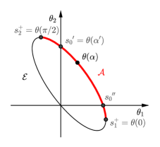
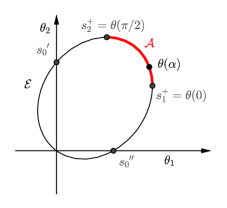
Figure 18. The arc $\mathcal{A}=[s_{1}^{+},s_{2}+]$ if $\theta_{1}(s_{2}^{+})<0$, $\theta_{2}(s_{1}^{+})<0$ on the left picture, if $\theta_{1}(s_{2}^{+})>0$, $\theta_{2}(s_{1}^{+})>0$ on the right picture

The important conclusion is that in all cases, the pole $p$ of $\varphi_{2}$ on the arc $\{s^{\prime}_{0},\theta(\alpha)\}$ with the smallest $\langle\theta(p)\mid e_{\alpha}\rangle$ is the closest to $s^{\prime}_{0}$. In the same way we can consider the arc $\{s^{\prime\prime}_{0},\theta(\alpha)\}$ and find out, due to monotonicity of the function $\langle\theta(s)\mid e_{\alpha}\rangle$, that the pole of $\varphi_{1}$ with the smallest $\langle\theta(p)\mid e_{\alpha}\rangle$ is the closest to $s^{\prime\prime}_{0}$. We know from Lemmas 12–15 the way that these poles are related to zeros of $\gamma_{1}$ and $\gamma_{2}$. Now we summarize this information in the following theorem.

Theorem 21.

• Let $\zeta\theta^{**}\not\in\{\theta(\alpha),s^{\prime}_{0}\}$, $\eta\theta^{*}\not\in\{\theta(\alpha),s^{\prime\prime}_{0})\}$. Then ${\cal P^{\prime}}_{\alpha}$ and ${\cal P^{\prime\prime}}_{\alpha}$ are both empty, $\theta(\alpha)$ is not a pole of $\varphi_{1}$ and neither of $\varphi_{2}$.

• Let $\zeta\theta^{**}\in\}\theta(\alpha),s^{\prime}_{0}\}$ and $\eta\theta^{*}\not\in\}\theta(\alpha),s^{\prime\prime}_{0}\}$. Then

  $$\min_{p\in{\cal P^{\prime}}_{\alpha}\cup{\cal P^{\prime\prime}}_{\alpha}}\langle\theta(p)\mid e_{\alpha}\rangle=\langle\zeta\theta^{**}\mid e_{\alpha}\rangle$$ (62)

  and this minimum over ${\cal P^{\prime}}_{\alpha}\cup{\cal P^{\prime\prime}}_{\alpha}$ is achieved at the unique element $p=\zeta\theta^{**}$ which is a pole of the first order of $\varphi_{2}$.

• Let $\zeta\theta^{**}\not\in\}\theta(\alpha),s^{\prime}_{0}\}$ and $\eta\theta^{*}\in\{s^{\prime\prime}_{0},\theta(\alpha)\{$. Then

  $$\min_{p\in{\cal P^{\prime}}_{\alpha}\cup{\cal P^{\prime\prime}}_{\alpha}}\langle\theta(p)\mid e_{\alpha}\rangle=\langle\eta\theta^{*}\mid e_{\alpha}\rangle$$ (63)

  and this minimum over ${\cal P^{\prime}}_{\alpha}\cup{\cal P^{\prime\prime}}_{\alpha}$ is achieved at the unique element $p=\eta\theta^{*}$ which is a pole of the first order of $\varphi_{1}$.

• Let $\zeta\theta^{**}\in\}\theta(\alpha),s^{\prime}_{0}\}$ and $\eta\theta^{*}\in\{s^{\prime\prime}_{0},\theta(\alpha)\{$.

  If $\langle\zeta\theta^{**}\mid e_{\alpha}\rangle<\langle\eta\theta^{*}\mid e_{\alpha}\rangle$, then (62) is valid. If $\langle\zeta\theta^{*}\mid e_{\alpha}\rangle>\langle\eta\theta^{**}\mid e_{\alpha}\rangle$, then (63) is valid. In both cases the minimum over ${\cal P^{\prime}}_{\alpha}\cup{\cal P^{\prime\prime}}_{\alpha}$ is achieved at the unique element which is the pole of the first order $p=\zeta\theta^{**}$ of $\varphi_{2}$ or the pole of the first order $p=\eta\theta^{*}$ of $\varphi_{1}$ respectively.

  If $\langle\zeta\theta^{**}\mid e_{\alpha}\rangle=\langle\eta\theta^{*}\mid e_{\alpha}\rangle$, then

  $$\min_{p\in{\cal P^{\prime}}_{\alpha}\cup{\cal P^{\prime\prime}}_{\alpha}}\langle\theta(p)\mid e_{\alpha}\rangle=\langle\zeta\theta^{**}\mid e_{\alpha}\rangle=\langle\eta\theta^{*}\mid e_{\alpha}\rangle.$$ (64)

  This minimum over ${\cal P^{\prime}}_{\alpha}\cup{\cal P^{\prime\prime}}_{\alpha}$ is achieved at exactly two elements $p=\zeta\theta^{**}$ and $p=\eta\theta^{*}$ which are poles of the first order of $\varphi_{1}$ and $\varphi_{2}$ respectively.

Proof.

(a) Let $\theta_{1}(s_{2}^{+})<0$ and let $\alpha>\alpha^{\prime}$ defined above. Then $\theta_{1}(\alpha)<0$ and all points of the arc $\{\theta(\alpha),s^{\prime}_{0}\{$ have the first coordinate negative, so that function $\varphi_{2}(\theta_{1}(s))$ is initially well defined at them and holomorphic. Let now $\theta_{1}(s_{2}^{+})<0$ and $\alpha\in]0,\alpha^{\prime}[$ or $\theta_{1}(s_{2}^{+})\geqslant 0$. Then $\theta_{1}(\alpha)>0$ and the arc $\{\theta(\alpha),s^{\prime}_{0}\}$ written in the anticlockwise direction is $[\theta(\alpha),s^{\prime}_{0}]$. Assume that $\varphi_{2}(\theta_{1}(s))$ has poles on $[\theta(\alpha),s^{\prime}_{0}[$ and $\theta^{p}$ is the closest to $s^{\prime}_{0}$. Then by Lemma 13 either $\gamma_{2}(\zeta\theta^{p})=0$ or parameters are such that $\theta_{2}(s_{1}^{+})>0$, $\eta\zeta\theta^{p}\in]\eta s_{1}^{+},s_{0}[$ and $\gamma_{1}(\eta\zeta\theta^{p})=0$. In the first case $\zeta\theta^{p}=\theta^{**}$ is a zero of $\gamma_{2}$ different from $s_{0}$. This implies $\theta^{p}=\zeta\theta^{**}\in[\theta(\alpha)s^{\prime}_{0}[$ which is impossible by assumptions. In the second case $\eta\zeta\theta^{p}=\theta^{*}$ is a zero of $\gamma_{1}$ different from $s_{0}$. This implies $\zeta\theta^{p}=\eta\theta^{*}\in\eta]\eta s_{1}^{+},s_{0}[=]s^{\prime\prime}_{0},s_{1}^{+}[\subset]s^{\prime\prime}_{0},\theta(\alpha)[=\}\theta(\alpha),s^{\prime\prime}_{0}\{$ that contradicts the assumptions as well. Hence $\varphi_{2}(\theta_{1}(s))$ has no poles on the open arc $\}\theta(\alpha),s^{\prime}_{0}\{$ and neither at $\theta(\alpha)$, ${\cal P^{\prime}}_{\alpha}$ is empty, The reasoning for ${\cal P^{\prime\prime}}_{\alpha}$ is the same.

(b) By stability conditions (1) and (2) $\theta^{**}_{1}>0$, then $\zeta\theta^{**}_{1}>0$. Thus $\theta_{1}(\alpha)>0$, in the case $\theta_{1}(s_{2}^{+})<0$ the angle $\alpha$ must be smaller than $\alpha^{\prime}$ and the arc $\}\theta(\alpha),s^{\prime}_{0}\{$ should be written $]\theta(\alpha),s^{\prime}_{0}[$. By Lemma 12 there exist poles of function $\varphi_{2}(\theta_{1}(s))$ on this arc and $\zeta\theta^{**}$ is one among them. By Lemma 13 $\zeta\theta^{**}$ can not be the closest pole to $s^{\prime}_{0}$ only if the parameters are such that $\theta_{2}(s_{1}^{+})>0$ and for some $\theta^{p}\in]\theta(\alpha),s^{\prime}_{0}[$ such that $\eta\zeta\theta^{p}\in]\eta s_{1}^{+},s_{0}[$ $\gamma_{1}(\eta\zeta\theta^{p})=0$. But then $\eta\zeta\theta^{p}=\theta^{*}$ is a zero of $\gamma_{1}$ different from $s_{0}$. It follows $\zeta\theta^{p}=\eta\theta^{*}\in\eta]\eta s_{1}^{+},s_{0}[=]s^{\prime\prime}_{0},s_{1}^{+}[\subset]s^{\prime\prime}_{0},\theta(\alpha)[=\}\theta(\alpha),s^{\prime\prime}_{0}\{$ that is impossible by assumptions. Hence by Lemma 13 $\zeta\theta^{**}$ is the closest pole to $s^{\prime}_{0}$ of $\varphi_{2}(\theta_{1}(s))$ and it is of the first order. The function $\langle\theta(s)\mid e_{\alpha}\rangle$ being decreasing on $]\theta(\alpha),s^{\prime}_{0}[$ when $s$ runs the arc in the anticlockwise direction, thus

$$\min_{p\in{\cal P^{\prime}}_{\alpha}}\langle\theta(p)\mid e_{\alpha}\rangle=\langle\zeta\theta^{**}\mid e_{\alpha}\rangle,$$ (65)

and the minimum is achieved on the unique element $\zeta\theta^{**}$.

If ${\cal P}^{\prime\prime}_{\alpha}$ is empty then the statement (b) is proved.

Assume that ${\cal P}^{\prime\prime}_{\alpha}$ is not empty. Then there exist poles of $\varphi_{1}(\theta_{2}(s))$ on the arc $\}\theta(\alpha),s^{\prime\prime}_{0}\{$. Since function $\varphi_{1}(\theta_{2}(s))$ is initially well defined and holomorphic at all points with the second coordinate negative, then $\theta_{2}(\alpha)>0$ and the arc is $]s^{\prime\prime}_{0},\theta(\alpha)[$ when written in the anticlockwise direction. Let $\theta^{p}$ be a pole of $\varphi_{1}(\theta_{2}(s))$ which is the closest to $s^{\prime\prime}_{0}$. Then by Lemma 13 either $\gamma_{1}(\eta\theta^{p})=0$ or parameters are such that $\theta_{1}(s_{2}^{+})>0$, $\zeta\eta\theta^{p}\in]s_{0},\zeta s_{2}^{+}[$ and $\gamma_{2}(\zeta\eta\theta^{p})=0$. In the first case $\eta\theta^{p}=\theta^{*}$ is a zero of $\gamma_{1}$ different from $s_{0}$. This implies $\theta^{p}=\eta\theta^{*}\in]s^{\prime\prime}_{0},\theta(\alpha)[$ which is impossible by assumptions. In the second case $\zeta\eta\theta^{p}=\theta^{**}$ where $\eta\theta^{p}=\zeta\theta^{**}\in\zeta]s_{0},\zeta s_{2}^{+}[=]s_{2}^{+},s^{\prime}_{0}[\subset]\theta(\alpha),s^{\prime}_{0}[$. Thus $\theta^{p}=\eta\zeta\theta^{**}$ is the closest pole to $s^{\prime\prime}_{0}$. Hence, the closest pole of the first order coincides with it or is further away from $s^{\prime\prime}_{0}$. Since the function $<\theta(s)\mid e_{\alpha}>$ is increasing on $]s^{\prime\prime}_{0},\theta(\alpha)[$ when $s$ is running from $s^{\prime\prime}_{0}$ to $\theta(\alpha)$, we derive

$$\min_{p\in{\cal P^{\prime\prime}}_{\alpha}}\langle\theta(p)\mid e_{\alpha}\rangle\geqslant\langle\eta\zeta\theta^{**}\mid e_{\alpha}\rangle.$$

But by Lemma 14

$$\theta_{1}(\eta\zeta\theta^{**})>\theta_{1}(\zeta\theta^{**}),\ \ \theta_{2}(\eta\zeta\theta^{**})=\theta_{2}(\zeta\theta^{**})$$

from where

$$\langle\eta\zeta\theta^{**}\mid e_{\alpha}\rangle>\langle\zeta\theta^{**}\mid e_{\alpha}\rangle.$$

Thus, whenever ${\cal P^{\prime\prime}}_{\alpha}$ is non empty,

$$\min_{p\in{\cal P^{\prime\prime}}_{\alpha}}\langle\theta(p)\mid e_{\alpha}\rangle>\langle\zeta\theta^{**}\mid e_{\alpha}\rangle.$$

This inequality combined with (65) finishes the proof of (b).

The proof of (c) is symmetric.

(d) Since $\theta^{*}_{2}=\eta\theta^{*}_{2}>0$ and $\theta^{**}_{1}=\zeta\theta^{**}_{1}>0$ by stability conditions (1) and (2), then $\theta(\alpha)$ has both coordinates positive. The corresponding arcs written in the anticlockwise direction are $]\theta(\alpha),s^{\prime}_{0}[\subset]s_{1}^{+},s^{\prime}_{0}[$ and $]s^{\prime\prime}_{0},\theta(\alpha)[\subset]s^{\prime\prime}_{0},s_{2}^{+}[$. By Lemma 13 $\zeta\theta^{**}$ is a pole of $\varphi_{2}(\theta_{1}(s))$ on the first of these arcs while $\eta\theta^{*}$ is a pole of $\varphi_{1}(\theta_{2}(s))$ on the second one. Then one of the statements of Lemma 15 (i), (ii) or (iii) holds true.

Under the statement (i), taking into account the monotonicity of the function $\langle\theta(s)\mid e_{\alpha}\rangle$ on the arcs, we derive immediately that $\min_{p\in{\cal P^{\prime}}_{\alpha}}\langle\theta(p)\mid e_{\alpha}\rangle=\langle\zeta\theta^{**}\mid e_{\alpha}\rangle$, and this minimum is achieved on the unique element $p=\zeta\theta^{**}$ . We derive also that $\min_{p\in{\cal P^{\prime\prime}}_{\alpha}}\langle\theta(p)\mid e_{\alpha}\rangle=\langle\eta\theta^{*}\mid e_{\alpha}\rangle$ and this minimum is achieved on the unique element $p=\eta\theta^{*}$. Thus, under the statement (i) of Lemma 15, the theorem is immediate.

Assume now (ii) of Lemma 15. Again by monotonicity of $\langle\theta(s)\mid e_{\alpha}\rangle$ we deduce $\min_{p\in{\cal P^{\prime}}_{\alpha}}\langle\theta(p)\mid e_{\alpha}\rangle=\langle\zeta\theta^{**}\mid e_{\alpha}\rangle$ where the minimum is achieved at the unique element $\zeta\theta^{**}$. Under (ii) all poles of $\varphi_{1}(\theta_{2}(s))$ on $]s^{\prime\prime}_{0},\theta(\alpha)[$ are not closer to $s^{\prime\prime}_{0}$ than $\eta\zeta\theta^{**}$ , so that either ${\cal P^{\prime\prime}}_{\alpha}$ is empty or

$$\min_{p\in{\cal P^{\prime\prime}}_{\alpha}}\langle\theta(p)\mid e_{\alpha}\rangle\geqslant\langle\eta\zeta\theta^{**}\mid e_{\alpha}\rangle.$$

By Lemma 14 $\theta_{1}(\eta\zeta\theta^{**})>\theta_{1}(\zeta\theta^{**}),$ $\theta_{2}(\eta\zeta\theta^{**})=\theta_{2}(\zeta\theta^{**})$ from where $\langle\eta\zeta\theta^{**}\mid e_{\alpha}\rangle>\langle\zeta\theta^{**}\mid e_{\alpha}\rangle$. Hence

$$\min_{p\in{\cal P^{\prime\prime}}_{\alpha}}\langle\theta(p)\mid e_{\alpha}\rangle>\langle\zeta\theta^{**}\mid e_{\alpha}\rangle,$$

and finally

$$\min_{p\in{\cal P^{\prime}}_{\alpha}\cup{\cal P^{\prime\prime}}_{\alpha}}\langle\theta(p)\mid e_{\alpha}\rangle=\langle\zeta\theta^{**}\mid e_{\alpha}\rangle$$ (66)

where the minimum is achieved on the unique element $\zeta\theta^{**}$. From the other hand, the pole $\eta\theta^{*}\in]s^{\prime\prime}_{0},\theta(\alpha)[$ of $\varphi_{1}(\theta_{2}(s))$ in this case is not closer to $s^{\prime\prime}_{0}$ than $\eta\zeta\theta^{**}$. Then the inequality

$$\langle\eta\theta^{*}\mid e_{\alpha}\rangle\geqslant\langle\eta\zeta\theta^{**}\mid e_{\alpha}\rangle>\langle\zeta\theta^{**}\mid e_{\alpha}\rangle$$ (67)

is valid.

Under the statement (iii) of Lemma 15, by symmetric arguments, $\min_{p\in{\cal P^{\prime}}_{\alpha}\cup{\cal P^{\prime\prime}}_{\alpha}}\langle\theta(p)\mid e_{\alpha}\rangle=\langle\eta\theta^{*}\mid e_{\alpha}\rangle$ where the minimum is achieved on the unique element $\eta\theta^{*}$, while $\langle\eta\theta^{*}\mid e_{\alpha}\rangle<\langle\zeta\theta^{**}\mid e_{\alpha}\rangle$. The concludes the proof of the lemma.

∎

5. Asymptotic expansion of the density $\pi(r\cos(\alpha),r\sin(\alpha))$, $r\to\infty$, $\alpha\in\mathcal{O}(\alpha_{0})$

5.1. Given angle $\alpha_{0}$, asymptotic expansion of the density as a function of parameters $(\Sigma,\mu,R)$

We are now ready to formulate and prove the results. In this section we fix an angle $\alpha_{0}\in]0,\pi/2[$ and give the asymptotic expansion of the density of stationary distribution depending on parameters $(\Sigma,\mu,R)$, and more precisely on the position of zeros of $\gamma_{1}$ and $\gamma_{2}$ on ellipse $\mathcal{E}$.

In the first theorem parameters $(\Sigma,\mu,R)$ are such that the asymptotic expansion is determined by the saddle-point.

Theorem 22.

Let $\alpha_{0}\in]0,\pi/2[$, $\mathcal{O}(\alpha_{0})$ is a small enough neighborhood of $\alpha_{0}$. Assume that $\zeta\theta^{**}\not\in\{\theta(\alpha_{0}),s^{\prime}_{0}\}$, $\eta\theta^{*}\not\in\{\theta(\alpha_{0}),s^{\prime\prime}_{0})\}$. Then there exist constants $c^{l}(\alpha)$, $l=0,1,2,\ldots$, such that for any $k>0$:

$$\pi(r\cos(\alpha),r\sin(\alpha))\sim\sum_{l=0}^{k}\frac{c^{l}(\alpha)}{r^{l}\sqrt{r}}e^{-r\langle\theta(\alpha)\mid e_{\alpha}\rangle},\ \hbox{ as }r\to\infty,\ \hbox{ uniformly for }\alpha\in\mathcal{O}(\alpha_{0}).$$ (68)

Constants $c^{l}(\alpha)$ $l=0,1,2,\ldots$ depend continuously on $\alpha$ and can be expressed in terms of functions $\varphi_{1}$ and $\varphi_{2}$ and their derivatives at $\theta(\alpha)$. Namely

$$c^{0}(\alpha)=c_{\theta_{1}}^{0}(\alpha)+c_{\theta_{2}}^{0}(\alpha)$$ (69)

where $c_{\theta_{1}}^{0}(\alpha)$ and $c_{\theta_{2}}^{0}(\alpha)$ are defined in Lemma 20.

Proof.

By Lemma 17 (iii) $\theta(\alpha)$ depends continuously on $\alpha$, then $\zeta\theta^{**}\not\in\{\theta(\alpha),s^{\prime}_{0}\}$, $\eta\theta^{*}\not\in\{\theta(\alpha),s^{\prime\prime}_{0}\}$ for all $\alpha\in\mathcal{O}(\alpha_{0})$. By Theorem 21 (a) the sets ${\cal P^{\prime}}_{\alpha}$ and ${\cal P^{\prime\prime}}_{\alpha}$ are both empty, furthermore, $\theta(\alpha)$ is not a pole of $\varphi_{1}$ and neither of $\varphi_{2}$. Then by Lemma 18 the density equals the sum of integrals along shifted contours $\Gamma_{\theta_{1},\alpha}$ and $\Gamma_{\theta_{2},\alpha}$ the asymptotics of which is found in Lemma 20, $c^{l}(\alpha)=c^{l}_{\theta_{1}}(\alpha)+c^{l}_{\theta_{2}}(\alpha)$, $l=0,1,2,\ldots$. ∎

In the second theorem parameters $(\Sigma,\mu,R)$ are such that the most important terms of the asymptotic expansion come from the poles of $\varphi_{1}$ or $\varphi_{2}$ and the smaller ones come from the saddle-point.

Theorem 23.

Let $\alpha_{0}\in]0,\pi/2[$, $\mathcal{O}(\alpha_{0})$ is a small enough neighborhood of $\alpha_{0}$. Assume that $\zeta\theta^{**}\in\}\theta(\alpha_{0}),s^{\prime}_{0}\}$ or $\eta\theta^{*}\in\}\theta(\alpha_{0}),s^{\prime\prime}_{0}\}$. Assume also that $\theta(\alpha_{0})$ is not a pole of $\varphi_{1}(\theta_{2}(s))$ neither of $\varphi_{2}(\theta_{1}(s))$. Then for any $k>0$ when $r\to\infty$, uniformly for $\alpha\in\mathcal{O}(\alpha_{0})$ we have

$$\pi(r\cos(\alpha),r\sin(\alpha)) \sim \sum_{p\in{\cal P^{\prime}}_{\alpha_{0}}}{\rm res}_{p}\varphi_{2}(\theta_{1}(s))\frac{\gamma_{2}(p)}{\sqrt{d(\theta_{1}(p))}}e^{-r\langle\theta(p)\mid e_{\alpha}\rangle}$$ (70)

$${}+\sum_{p\in{\cal P^{\prime\prime}}_{\alpha_{0}}}{\rm res}_{p}\varphi_{1}(\theta_{2}(s))\frac{\gamma_{1}(p)}{\sqrt{\tilde{d}(\theta_{2}(p))}}e^{-r\langle\theta(p)\mid e_{\alpha}\rangle}$$

$${}+\sum_{l=0}^{k}\frac{c^{l}(\alpha)}{r^{l}\sqrt{r}}e^{-r\langle\theta(\alpha)\mid e_{\alpha}\rangle}.$$

Constants $c^{l}(\alpha)$ $l=0,1,2,\ldots$ are the same as in Theorem 22. Furthermore

• If $\zeta\theta^{**}\in\}\theta(\alpha_{0}),s^{\prime}_{0}\}$ and $\eta\theta^{*}\not\in\}\theta(\alpha_{0}),s^{\prime\prime}_{0}\}$, then the main term in the expansion (70) is at $p=\zeta\theta^{**}$.

• If If $\zeta\theta^{**}\not\in\}\theta(\alpha_{0}),s^{\prime}_{0}\}$ and $\eta\theta^{*}\in\}\theta(\alpha_{0}),s^{\prime\prime}_{0}\}$, then the main term in (70) is at $p=\eta\theta^{*}$.

• Let $\zeta\theta^{**}\in\}\theta(\alpha_{0}),s^{\prime}_{0}\}$ and $\eta\theta^{*}\in\}\theta(\alpha_{0}),s^{\prime\prime}_{0}\}$. If $\langle\zeta\theta^{**}\mid e_{\alpha_{0}}\rangle<\langle\eta\theta^{*}\mid e_{\alpha_{0}}\rangle$, then the main term in (70) is at $p=\zeta\theta^{**}$.

  If $\langle\zeta\theta^{**}\mid e_{\alpha_{0}}\rangle>\langle\eta\theta^{*}\mid e_{\alpha_{0}}\rangle$, then main term in (70) is at $p=\eta\theta^{*}$.

  If $\langle\zeta\theta^{**}\mid e_{\alpha_{0}}\rangle=\langle\eta\theta^{*}\mid e_{\alpha_{0}}\rangle$, then two the most important terms in the expansion (70) are at $p=\zeta\theta^{**}$ and at $p=\eta\theta^{*}$.

Proof.

Point $\theta(\alpha_{0})$ being not a pole of $\varphi_{1}$ neither of $\varphi_{2}$, one can choose $\mathcal{O}(\alpha_{0})$ small enough such that $\theta(\alpha)$ is not a pole of no one of these functions and $\mathcal{P}^{\prime}_{\alpha}\cup\mathcal{P}^{\prime\prime}_{\alpha}=\mathcal{P}^{\prime}_{\alpha_{0}}\cup\mathcal{P}^{\prime\prime}_{\alpha_{0}}$ for all $\alpha\in\mathcal{O}(\alpha_{0})$. By assumptions $\zeta\theta^{**}\in\}\theta(\alpha_{0}),s^{\prime}_{0}\}$ or $\eta\theta^{*}\in\}\theta(\alpha_{0}),s^{\prime\prime}_{0}\}$, then by Theorem 21 (b), (c) or (d) $\mathcal{P}^{\prime}_{\alpha_{0}}\cup\mathcal{P}^{\prime\prime}_{\alpha_{0}}$ is not empty. Finally by virtue of Lemma 18 and Lemma 20 the representation (70) holds true.

Let us study the main asymptotic term. Statements (i), (ii) and (iii) for $\alpha=\alpha_{0}$ follow directly from Theorem 21 (b), (c) and (d). They remain valid for any $\alpha\in\mathcal{O}(\alpha_{0})$ due to the continuity of the functions $\alpha\to\langle\theta(p)\mid e_{\alpha}\rangle$ for any $p\in\mathcal{P}^{\prime}_{\alpha_{0}}\cup\mathcal{P}^{\prime\prime}_{\alpha_{0}}$. ∎

Remark. Under parameters such that $\zeta\theta^{**}\in\}\theta(\alpha_{0}),s^{\prime}_{0}\}$, $\eta\theta^{*}\in\}\theta(\alpha_{0}),s^{\prime\prime}_{0}\}$ and $\langle\zeta\theta^{**}\mid e_{\alpha_{0}}\rangle=\langle\eta\theta^{*}\mid e_{\alpha_{0}}\rangle$ (case (iii)), for any fixed angle $\alpha<\alpha_{0}$, the main asymptotic term is at $\eta\theta^{*}$ and the second one is at $\zeta\theta^{**}$; for any fixed angle $\alpha>\alpha_{0}$ the pole $\zeta\theta^{**}$ provides the main asymptotic term and $\eta\theta^{*}$ gives the second one. If $r\to\infty$ and $\alpha\to\alpha_{0}$, both of these terms should be taken into account.

In Theorem 23 $\theta(\alpha_{0})$ is assumed not to be a pole of $\varphi_{1}$ and neither of $\varphi_{2}$, that is why Lemma 18 applies. Nevertheless, it may happen (for a very few angles and under some sets of parameters) that $\theta(\alpha_{0})$ is a pole of one of these functions. In this case the following theorem holds true.

Theorem 24.

Let $\alpha_{0}\in]0,\pi/2[$. Assume that $\zeta\theta^{**}\in\}\theta(\alpha_{0}),s^{\prime}_{0}\}$ or $\eta\theta^{*}\in\}\theta(\alpha_{0}),s^{\prime\prime}_{0})\}$.

Assume also that $\theta(\alpha_{0})$ is a pole of $\varphi_{1}(\theta_{2}(s))$ or of $\varphi_{2}(\theta_{1}(s))$.

Then for any $\delta>0$ there exists a small enough neighborhood $\mathcal{O}(\alpha_{0})$ such that

$$\pi(r\cos(\alpha),r\sin(\alpha)) \sim \sum_{p\in{\cal P^{\prime}}_{\alpha_{0}}}{\rm res}_{p}\varphi_{2}(\theta_{1}(s))\frac{\gamma_{2}(p)}{\sqrt{d(\theta_{1}(p))}}e^{-r\langle\theta(p)\mid e_{\alpha}\rangle}$$ (71)

$${}+\sum_{p\in{\cal P^{\prime\prime}}_{\alpha_{0}}}{\rm res}_{p}\varphi_{1}(\theta_{2}(s))\frac{\gamma_{1}(p)}{\sqrt{\tilde{d}(\theta_{2}(p))}}e^{-r\langle\theta(p)\mid e_{\alpha}\rangle}$$

$${}+o(e^{-r(\langle\theta(\alpha)\mid e_{\alpha}\rangle-\delta)})\ \ \ r\to\infty,\hbox{ uniformly }\forall\alpha\in\mathcal{O}(\alpha_{0})$$

Furthermore, the main term in this expansion is the same as in Theorem 23, cases (i), (ii) and (iii).

Proof.

For any $\delta>0$ one can choose $\tau^{\prime}\in\}s^{\prime}_{0},\theta(\alpha_{0})\{$ and $\tau^{\prime\prime}\in\}s^{\prime\prime}_{0},\theta(\alpha_{0})\{$ close enough to $\theta(\alpha_{0})$ so that $\mathcal{P}^{\prime}_{\alpha_{0}}\subset\}s^{\prime}_{0},\tau^{\prime}\{$ and $\mathcal{P}^{\prime\prime}_{\alpha_{0}}\subset\}s^{\prime\prime}_{0},\tau"\{$. Furthermore $\tau^{\prime}$ and $\tau^{\prime\prime}$ can be chosen close enough to $\alpha_{0}$ so that $\langle\theta(\alpha_{0})\mid e_{\alpha_{0}}\rangle-\langle\tau^{\prime}\mid e_{\alpha_{0}}\rangle<\delta/4$ and $\langle\theta(\alpha_{0})\mid e_{\alpha_{0}}\rangle-\langle\tau^{\prime\prime}\mid e_{\alpha_{0}}\rangle<\delta/4$. Then by continuity of the functions $\alpha\to\langle\theta(\alpha)\mid e_{\alpha}\rangle$, $\alpha\to\langle\tau^{\prime}\mid e_{\alpha}\rangle$, $\alpha\to\langle\tau^{\prime\prime}\mid e_{\alpha}\rangle$ one can fix a small enough neighborhood $\mathcal{O}(\alpha_{0})$ such that

$$\langle\theta(\alpha)\mid e_{\alpha}\rangle-\langle\tau^{\prime}\mid e_{\alpha}\rangle<\delta/2,\ \ \ \langle\theta(\alpha)\mid e_{\alpha}\rangle-\langle\tau^{\prime\prime}\mid e_{\alpha}\rangle<\delta/2,\ \ \forall\alpha\in\mathcal{O}(\alpha_{0}).$$ (72)

Next, we shift the integration contours in (49) $\mathcal{I}_{\theta_{1}}^{+}$ and $\mathcal{I}_{\theta_{2}}^{+}$ to the new ones $\Gamma^{\prime}_{\theta_{1},\alpha}$ and $\Gamma^{\prime\prime}_{\theta_{2},\alpha}$ going through $\tau^{\prime}$ and $\tau^{\prime\prime}$ respectively that we construct as follows: $\Gamma^{\prime}_{\theta_{1},\alpha}=\Gamma^{\prime 1}_{\theta_{1},\alpha}\cup\Gamma^{\prime 2,\pm}_{\theta_{1},\alpha}\cup\Gamma^{\prime 3,\pm}_{\theta_{1},\alpha}$ where $\Gamma^{\prime 1}_{\theta_{1}}=\{s:\Re\theta_{1}(s)=\Re\theta_{1}(\tau^{\prime}),-V(\alpha)\leqslant\Im\theta_{1}(s)\leqslant V(\alpha)\}$, $\Gamma^{\prime 2,\pm}_{\theta_{1},\alpha}=\{s:\Im\theta_{1}(s)=\pm V(\alpha),0\leqslant\Re\theta_{1}(s)\leqslant\Re\theta_{1}(\tau^{\prime})\}$ if $\Re\theta_{1}(\tau^{\prime})>0$ and $\Gamma^{\prime 2,\pm}_{\theta_{1},\alpha}=\{s:\Im\theta_{1}(s)=\pm V(\alpha),0\geqslant\Re\theta_{1}(s)\geqslant\Re\theta_{1}(\tau^{\prime})\}$ if $\Re\theta_{1}(\tau^{\prime})<0$ , finally $\Gamma^{\prime 3,+}_{\theta_{1},\alpha}=\{s:\Re\theta_{1}(s)=0,\Im\theta_{1}(s)\geqslant V(\alpha)\}$, $\Gamma^{\prime 3,-}_{\theta_{1},\alpha}=\{s:\Re\theta_{1}(s)=0,\Im\theta_{1}(s)\leqslant-V(\alpha)\}$. The construction of $\Gamma^{\prime\prime}_{\theta_{2},\alpha}$ is analogous. The value $V(\alpha)$ is fixed as:

$$V(\alpha)=\max\Big{(}V,\frac{\langle\tau^{\prime}\mid e_{\alpha}\rangle-d_{1}}{d_{2}\sin(\alpha)},\frac{\langle\tau^{\prime\prime}\mid e_{\alpha}\rangle-d_{1}}{d_{2}\sin(\alpha)}\Big{)}$$ (73)

with notations from Lemma 19. Thanks to the representation (49) and Cauchy theorem

$$\pi(re_{\alpha})=\sum_{p\in{\cal P^{\prime}}_{\alpha_{0}}}{\rm res}_{p}\varphi_{2}(\theta_{1}(s))\frac{\gamma_{2}(p)}{\sqrt{d(\theta_{1}(p))}}e^{-r\langle\theta(p)\mid e_{\alpha}\rangle}+\sum_{p\in{\cal P^{\prime\prime}}_{\alpha_{0}}}{\rm res}_{p}\varphi_{1}(\theta_{2}(s))\frac{\gamma_{1}(p)}{\sqrt{\tilde{d}(\theta_{2}(p))}}e^{-r\langle\theta(p)\mid e_{\alpha}\rangle}$$

$${}+\frac{1}{2\pi\sqrt{\det\Sigma}}\int_{\Gamma^{\prime}_{\theta_{1},\alpha}}\frac{\varphi_{2}(s)\gamma_{2}(\theta(s))}{s}e^{-r\langle\theta(s)\mid e_{\alpha}\rangle}{\mathrm{d}s}+\frac{1}{2\pi\sqrt{\det\Sigma}}\int_{\Gamma^{\prime\prime}_{\theta_{2},\alpha}}\frac{\varphi_{1}(s)\gamma_{1}(\theta(s))}{s}e^{-r\langle\theta(s)\mid e_{\alpha}\rangle}\mathrm{d}s.$$ (74)

Applying Lemma 19 (i) for the estimation of integrals along $\Gamma^{\prime 1}_{\theta_{1},\alpha}$ and $\Gamma^{\prime\prime 1}_{\theta_{1},\alpha}$, and the same lemma (ii) for the estimation of those along $\Gamma^{\prime\pm 2}_{\theta_{1},\alpha}$ $\Gamma^{\prime\prime\pm 2}_{\theta_{2},\alpha}$, $\Gamma^{\prime\pm 3}_{\theta_{1},\alpha}$ and $\Gamma^{\prime\prime\pm 3}_{\theta_{2},\alpha}$ exactly as in Lemma 20 and in view of (73) we can show that with some constant $C>0$

$$\Big{|}\int_{\Gamma^{\prime}_{\theta_{1},\alpha}}\frac{\varphi_{2}(s)\gamma_{2}(\theta(s))}{s}e^{-r\langle\theta(s)\mid e_{\alpha}\rangle}{\mathrm{d}s}\Big{|} \leqslant Ce^{-r\langle\tau^{\prime}\mid e_{\alpha}\rangle},$$

$$\Big{|}\int_{\Gamma^{\prime\prime}_{\theta_{1},\alpha}}\frac{\varphi_{2}(s)\gamma_{2}(\theta(s))}{s}e^{-r\langle\theta(s)\mid e_{\alpha}\rangle}{\mathrm{d}s}\Big{|} \leqslant Ce^{-r\langle\tau^{\prime\prime}\mid e_{\alpha}\rangle}\ \ \forall r>0,\forall\alpha\in\mathcal{O}(\alpha_{0}).$$

Hence, by (72)

$$\int_{\Gamma^{\prime}_{\theta_{1},\alpha}}\frac{\varphi_{2}(s)\gamma_{2}(\theta(s))}{s}e^{-r\langle\theta(s)\mid e_{\alpha}\rangle}{\mathrm{d}s}+\int_{\Gamma^{\prime\prime}_{\theta_{2},\alpha}}\frac{\varphi_{1}(s)\gamma_{1}(\theta(s))}{s}e^{-r\langle\theta(s)\mid e_{\alpha}\rangle}\mathrm{d}s=o(e^{-r(\langle\theta(\alpha)\mid e_{\alpha}\rangle-\delta)})$$ (75)

as $r\to\infty$ uniformly $\forall\alpha\in\mathcal{O}(\alpha_{0})$. This finishes the proof of the representation (71). The analysis of the main term is the same as in Theorem 23. ∎

It remains to study the cases of parameters such that

• $\zeta\theta^{**}=\theta(\alpha_{0})$ and $\eta\theta^{*}\not\in\{s^{\prime\prime}_{0},\theta(\alpha_{0})\{$

• $\eta\theta^{*}=\theta(\alpha_{0})$ and $\zeta\theta^{**}\not\in\{s^{\prime\prime}_{0},\theta(\alpha_{0})\{$.

By Lemma 12 this means that $\theta(\alpha_{0})$ is a pole of one of functions $\varphi_{1}$ or $\varphi_{2}$. Since in both cases $\eta\theta^{*}\not\in\{s^{\prime\prime}_{0},\theta(\alpha)\{$, $\zeta\theta^{**}\not\in\{s^{\prime\prime}_{0},\theta(\alpha)\{$, we derive by the same reasoning as in Theorem 21 (a) that $\mathcal{P}^{\prime}_{\alpha_{0}}\cup\mathcal{P}^{\prime\prime}_{\alpha_{0}}$ is empty. The following theorem is valid.

Theorem 25.

Assume that $\alpha_{0}$ is such that the assumptions on parameters (O1) or (O2) are valid. Then for any $\delta>0$ there exists a small enough neighborhood $\mathcal{O}(\alpha_{0})$ such that

$$\pi(r\cos(\alpha),r\sin(\alpha))=o(e^{-r(\langle\theta(\alpha)\mid e_{\alpha}\rangle-\delta)})\ \ \ r\to\infty,\hbox{ uniformly }\forall\alpha\in\mathcal{O}(\alpha_{0}).$$ (76)

Proof.

We choose $\tau^{\prime}$ and $\tau^{\prime\prime}$ according to (72) and proceed exactly as in the proof of Theorem 24. ∎

Remark. In Theorems 24 and 25 $\theta(\alpha_{0})$ is a pole of one of the functions $\varphi_{1}$ or $\varphi_{2}$, hence at least one of the integrals (49) can not be shifted to $\Gamma_{\theta_{1},\alpha_{0}}$ or $\Gamma_{\theta_{2},\alpha_{0}}$ going through $\theta(\alpha_{0})$. Furthermore, although for any $\alpha\in\mathcal{O}(\alpha_{0})$, $\alpha\neq\alpha_{0}$, this shift is possible, the uniform asymptotic expansion by the saddle-point method as in Lemma 20 does not stay valid, that is why we are not able to specify small asymptotic terms in Theorem 24 neither to obtain a more precise result in Theorem 25. This should be possible if we consider the double asymptotics $r\to\infty$ and $\alpha\to\alpha_{0}$ and apply the (more advanced) saddle-point method in the special case when the saddle-point is approaching a pole of the integrand. We do not do it in the present paper.

Remark. Assumptions of theorems 22 — 25 are expressed in terms of positions on ellipse $\mathcal{E}$ of points $\zeta\theta^{**}$ and $\eta\theta^{*}$ that are images of zeros of $\gamma_{1}$ and $\gamma_{2}$ on $\mathcal{E}$ by Galois automorphisms. They can be also expressed in terms of the following simple inequalities.

Under parameters such that $\theta_{1}(\alpha_{0})>0$, we have $\zeta\theta^{**}\neq\{s^{\prime}_{0},\theta(\alpha_{0})\}$ iff $\theta^{**}\neq\{s_{0},\zeta\theta(\alpha_{0})\}$ that is equivalent to $\gamma_{2}(\zeta\theta(\alpha))<0$. Under parameters such that $\theta_{1}(\alpha_{0})\leqslant 0$, we have always $\zeta\theta^{**}\neq\{s^{\prime}_{0},\theta(\alpha_{0})\}$ because $\theta_{1}(\zeta\theta^{**})>0$ by stability conditions, in this case we have also $\gamma_{2}(\zeta\theta(\alpha_{0}))\geqslant 0$. We come to the following conclusions.

• Assumption $\zeta\theta^{**}\neq\{s^{\prime}_{0},\theta(\alpha_{0})\}$ is equivalent to the one that $\gamma_{2}(\zeta\theta(\alpha_{0}))<0$ or $\theta_{1}(\alpha_{0})\leqslant 0$.

  Assumption $\zeta\theta^{**}\in\{s^{\prime}_{0},\theta(\alpha_{0})\{$ is equivalent to the one that $\gamma_{2}(\zeta\theta(\alpha_{0}))>0$ and $\theta_{1}(\alpha_{0})>0$.

• Assumption $\eta\theta^{*}\neq\{s^{\prime\prime}_{0},\theta(\alpha_{0})\}$ is equivalent to the one that $\gamma_{1}(\eta\theta(\alpha_{0}))<0$ or $\theta_{2}(\alpha_{0})\leqslant 0$.

  Assumption $\eta\theta^{**}\in\{s^{\prime\prime}_{0},\theta(\alpha_{0})\{$ is equivalent to the one that $\gamma_{1}(\eta\theta(\alpha_{0}))>0$ and $\theta_{2}(\alpha_{0})>0$.

5.2. Given parameters $(\Sigma,\mu,R)$, density asymptotics for all angles $\alpha_{0}\in]0,\pi/2[$

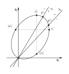
Figure 19. Theorem 26 case (i)

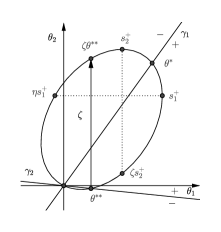
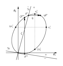
Figure 20. Theorem 26 case (iia) and (iva)

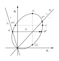
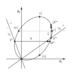
Figure 21. Theorem 26 case (iiia) and (ivb)

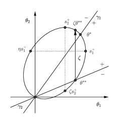
Figure 22. Theorem 26 case (iib)

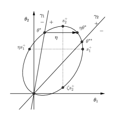
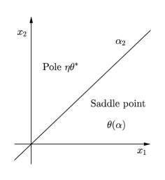
Figure 23. Theorem 26 case (iiib)

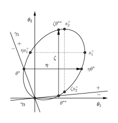
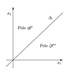
Figure 24. Theorem 26 case (ivc)

In this section we state the asymptotics of the density for all angles $\alpha_{0}\in]0,\pi/2[$ once parameters $(\Sigma,\mu,R)$ are fixed. Theorems 26 – 28 below are direct corollaries of Theorems 22 – 25 and elementary geometric properties of ellipse $\mathcal{E}$ and straight lines $\gamma_{1}(\theta)=0$ and $\gamma_{2}(\theta)=0$, therefore we do not give their proofs. To shorten the presentation, we restrict ourselves to the main term in the formulations of the results, although of course further terms of the expansions could be written. The different cases of Theorem 26 are illustrated by Figures 19–25.

Theorem 26.

Let $\theta_{1}(s_{2}^{+})>0$, $\theta_{2}(s_{1}^{+})>0$.

• Let $\gamma_{2}(s_{1}^{+})\leqslant 0$ and $\gamma_{1}(s_{2}^{+})\leqslant 0$ Then for any $\alpha_{0}\in]0,\pi/2[$ we have :

  $$\pi(r\cos\alpha,r\sin\alpha)\sim\frac{c(\alpha_{0})}{\sqrt{r}}\exp(-r\langle\theta(\alpha)\mid e_{\alpha}\rangle),\ \ r\to\infty,\alpha\to\alpha_{0},$$ (77)

  where the constant $c(\alpha_{0})$ depends continuously on $\alpha_{0}\in]0,\pi/2[$ and $\lim_{\alpha_{0}\to 0}c(\alpha_{0})=\lim_{\alpha_{0}\to\pi/2}c(\alpha_{0})=0$.

• Let $\gamma_{2}(s_{1}^{+})>0$ and $\gamma_{1}(s_{2}^{+})\leqslant 0$.

  • Let $\gamma_{2}(\zeta s_{2}^{+})\geqslant 0$ or equivalently $\frac{d\Theta_{2}^{+}(\theta_{1})}{d\theta_{1}}\Bigm{|}_{\theta_{1}^{**}}\geqslant 0$. Then for any $\alpha_{0}\in]0,\pi/2[$ we have

    $$\pi(r\cos\alpha,r\sin\alpha)\sim d_{1}\exp(-r\langle\zeta\theta^{**}\mid e_{\alpha}\rangle),\ \ r\to\infty,\alpha\to\alpha_{0},$$ (78)

    with some constant $d_{1}>0$.

  • Let $\gamma_{2}(\zeta s_{2}^{+})<0$ or equivalently $A^{**}\equiv\frac{d\Theta_{2}^{+}(\theta_{1})}{d\theta_{1}}\Bigm{|}_{\theta_{1}^{**}}<0$. Define $\alpha_{1}=\arctan(-1/A^{**})\in]0,\pi/2[$. Then for any $\alpha_{0}\in]0,\alpha_{1}[$ we have (78) and for any $\alpha\in]\alpha_{1},\pi/2[$ we have (77).

• Let $\gamma_{2}(s_{1}^{+})<0$ and $\gamma_{1}(s_{2}^{+})\geqslant 0$.

  • Let $\gamma_{1}(\eta s_{1}^{+})\geqslant 0$ or equivalently $\frac{d\Theta_{1}^{+}(\theta_{2})}{d\theta_{2}}\Bigm{|}_{\theta_{2}^{*}}\geqslant 0$. Then for any $\alpha_{0}\in]0,\pi/2[$ we have

    $$\pi(r\cos\alpha,r\sin\alpha)\sim d_{2}\exp(-r\langle\eta\theta^{*}\mid e_{\alpha}\rangle),\ \ r\to\infty,\alpha\to\alpha_{0},$$ (79)

    with some constant $d_{2}>0$.

  • Let $\gamma_{1}(\eta s_{1}^{+})<0$ or equivalently $A^{*}\equiv\frac{d\Theta_{1}^{+}(\theta_{2})}{d\theta_{2}}\Bigm{|}_{\theta_{2}^{*}}<0$. Define $\alpha_{2}=\arctan(-A^{*})\in]0,\pi/2[$. Then for any $\alpha_{0}\in]0,\alpha_{2}[$ we have (77) and for any $\alpha\in]\alpha_{2},\pi/2[$ we have (79).

• Let $\gamma_{2}(s_{1}^{+})>0$ and $\gamma_{1}(s_{2}^{+})>0$.

  • Let $\theta_{1}(\zeta\theta^{**})\leqslant\theta_{1}(\eta\theta^{*})$ and $\theta_{2}(\zeta\theta^{**})\leqslant\theta_{2}(\eta\theta^{*})$ where at least one of inequalities is strict. Then for any $\alpha_{0}\in]0,\pi/2[$ we have (78).

  • Let $\theta_{1}(\zeta\theta^{**})\geqslant\theta_{1}(\eta\theta^{*})$ and $\theta_{2}(\zeta\theta^{**})\geqslant\theta_{2}(\eta\theta^{*})$ where at least one of inequalities is strict. Then for any $\alpha\in]0,\pi/2[$ we have (79).

  • Let $\theta_{1}(\zeta\theta^{**})\leqslant\theta_{1}(\eta\theta^{*})$ and $\theta_{2}(\zeta\theta^{**})\geqslant\theta_{2}(\eta\theta^{*})$ where at least one of the inequalities is strict. Let us define $\beta_{0}=\arctan\frac{\theta_{1}(\zeta\theta^{**})-\theta_{1}(\eta\theta^{*})}{\theta_{2}(\eta\theta^{*})-\theta_{2}(\zeta\theta^{**})}$ Then for any $\alpha_{0}\in]0,\beta_{0}[$ we have (78), for any $\alpha_{0}\in]\beta_{0},\pi/2[$ we have (79) and for $\alpha_{0}=\beta_{0}$ we have

    $$\pi(r\cos\alpha,r\sin\alpha)\sim d_{1}\exp(-r\langle\zeta\theta^{**}\mid e_{\alpha}\rangle)+d_{2}\exp(-r\langle\eta\theta^{*}\mid e_{\alpha}\rangle),\ \ r\to\infty,\alpha\to\alpha_{0}.$$ (80)

  • Let $\theta_{1}(\zeta\theta^{**})\geqslant\theta_{1}(\eta\theta^{*})$ and $\theta_{2}(\zeta\theta^{**})\leqslant\theta_{2}(\eta\theta^{*})$. Let us define angles $\alpha_{1}$ and $\alpha_{2}$ as in (ii) and (iii). Then $0<\alpha_{1}\leqslant\alpha_{2}<\pi/2$; for any $\alpha_{0}\in]0,\alpha_{1}[$ we have (78) , for any $\alpha_{0}\in]\alpha_{1},\alpha_{2}[$ we have (77) and for any $\alpha_{0}\in]\alpha_{2},\pi/2[$ we have (79).

Theorem 27.

Let $\theta_{1}(s_{2}^{+})\leqslant 0$, $\theta_{2}(s_{1}^{+})\leqslant 0$.

• Let $\gamma_{2}(s_{1}^{+})\leqslant 0$ and $\gamma_{1}(s_{2}^{+})\leqslant 0$ Then for any $\alpha_{0}\in]0,\pi/2[$ the asymptotics (77) is valid.

• Let $\gamma_{2}(s_{1}^{+})>0$ and $\gamma_{1}(s_{2}^{+})\leqslant 0$. Let $A^{**}\equiv\frac{d\Theta_{2}^{+}(\theta_{1})}{d\theta_{1}}\Bigm{|}_{\theta_{1}^{**}}$. Then $\alpha_{1}=\arctan(-1/A^{**})\in]0,\pi/2[$. For any $\alpha_{0}\in]0,\alpha_{1}[$ the asymptotics (78) is valid and and for any $\alpha\in]\alpha_{1},\pi/2[$ the asymptotics (77) holds true.

• Let $\gamma_{2}(s_{1}^{+})<0$ and $\gamma_{1}(s_{2}^{+})\geqslant 0$. Let $A^{*}\equiv\frac{d\Theta_{1}^{+}(\theta_{2})}{d\theta_{2}}\Bigm{|}_{\theta_{2}^{*}}$. Then $\alpha_{2}=\arctan(-A^{*})\in]0,\pi/2[$. For any $\alpha_{0}\in]0,\alpha_{2}[$ the asymptotics (77) is valid and for any $\alpha\in]\alpha_{2},\pi/2[$ the asymptotics (79) holds true.

• Let $\gamma_{2}(s_{1}^{+})>0$ and $\gamma_{1}(s_{2}^{+})>0$. Then either $\theta_{1}(\zeta\theta^{**})<\theta_{1}(\eta\theta^{*})$ and $\theta_{2}(\zeta\theta^{**})>\theta_{2}(\eta\theta^{*})$, or $\theta_{1}(\zeta\theta^{**})>\theta_{1}(\eta\theta^{*})$ and $\theta_{2}(\zeta\theta^{**})<\theta_{2}(\eta\theta^{*})$, or finally $\theta_{1}(\zeta\theta^{**})=\theta_{1}(\eta\theta^{*})$ and $\theta_{2}(\zeta\theta^{**})=\theta_{2}(\eta\theta^{*})$.

  • Let $\theta_{1}(\zeta\theta^{**})<\theta_{1}(\eta\theta^{*})$ and $\theta_{2}(\zeta\theta^{**})>\theta_{2}(\eta\theta^{*})$. Let us define $\beta_{0}=\arctan\frac{\theta_{1}(\zeta\theta^{**})-\theta_{1}(\eta\theta^{*})}{\theta_{2}(\eta\theta^{*})-\theta_{2}(\zeta\theta^{**})}$ Then for any $\alpha_{0}\in]0,\beta_{0}[$ we have (78), for any $\alpha_{0}\in]\beta_{0},\pi/2[$ we have (79) and for $\alpha_{0}=\beta_{0}$ we have (80).

  • Let $\theta_{1}(\zeta\theta^{**})>\theta_{1}(\eta\theta^{*})$ and $\theta_{2}(\zeta\theta^{**})<\theta_{2}(\eta\theta^{*})$ or $\theta_{1}(\zeta\theta^{**})=\theta_{1}(\eta\theta^{*})$ and $\theta_{2}(\zeta\theta^{**})=\theta_{2}(\eta\theta^{*})$ Let us define angles $\alpha_{1}$ and $\alpha_{2}$ as in (ii) and (iii). Then $0<\alpha_{1}\leqslant\alpha_{2}<\pi/2$; for any $\alpha_{0}\in]0,\alpha_{1}[$ we have (78) , for any $\alpha_{0}\in]\alpha_{1},\alpha_{2}[$ we have (77) and for any $\alpha_{0}\in]\alpha_{2},\pi/2[$ we have (79).

Theorem 28.

Let $\theta_{1}(s_{2}^{+})>0$, $\theta_{2}(s_{1}^{+})\leqslant 0$.

• Let $\gamma_{2}(s_{1}^{+})\leqslant 0$ and $\gamma_{1}(s_{2}^{+})\leqslant 0$ Then for any $\alpha_{0}\in]0,\pi/2[$ the asymptotics (77) is valid.

• Let $\gamma_{2}(s_{1}^{+})>0$ and $\gamma_{1}(s_{2}^{+})\leqslant 0$.

  • Let $\gamma_{2}(\zeta s_{2}^{+})\geqslant 0$ or equivalently $\frac{d\Theta_{2}^{+}(\theta_{1})}{d\theta_{1}}\Bigm{|}_{\theta_{1}^{**}}\geqslant 0$. Then for any $\alpha_{0}\in]0,\pi/2[$ the asymptotics (78) is valid.

  • Let $\gamma_{2}(\zeta s_{2}^{+})<0$ or equivalently $A^{**}\equiv\frac{d\Theta_{2}^{+}(\theta_{1})}{d\theta_{1}}\Bigm{|}_{\theta_{1}^{**}}<0$. Define $\alpha_{1}=\arctan(-1/A^{**})\in]0,\pi/2[$. Then for any $\alpha_{0}\in]0,\alpha_{1}[$ we have (78) and for any $\alpha\in]\alpha_{1},\pi/2[$ we have (77).

• Let $\gamma_{2}(s_{1}^{+})<0$ and $\gamma_{1}(s_{2}^{+})\geqslant 0$. Let $A^{*}\equiv\frac{d\Theta_{1}^{+}(\theta_{2})}{d\theta_{2}}\Bigm{|}_{\theta_{2}^{*}}$. Then $\alpha_{2}=\arctan(-A^{*})\in]0,\pi/2[$. For any $\alpha_{0}\in]0,\alpha_{2}[$ the asymptotics (77) is valid and for any $\alpha\in]\alpha_{2},\pi/2[$ the asymptotics (79) holds true.

• Let $\gamma_{2}(s_{1}^{+})>0$ and $\gamma_{1}(s_{2}^{+})>0$. Then either $\theta_{1}(\zeta\theta^{**})\leqslant\theta_{1}(\eta\theta^{*})$ and $\theta_{2}(\zeta\theta^{**})\leqslant\theta_{2}(\eta\theta^{*})$, or $\theta_{1}(\zeta\theta^{**})<\theta_{1}(\eta\theta^{*})$ and $\theta_{2}(\zeta\theta^{**})>\theta_{2}(\eta\theta^{*})$, or $\theta_{1}(\zeta\theta^{**})>\theta_{1}(\eta\theta^{*})$ and $\theta_{2}(\zeta\theta^{**})<\theta_{2}(\eta\theta^{*})$, or finally $\theta_{1}(\zeta\theta^{**})=\theta_{1}(\eta\theta^{*})$ and $\theta_{2}(\zeta\theta^{**})=\theta_{2}(\eta\theta^{*})$.

  • Let $\theta_{1}(\zeta\theta^{**})\leqslant\theta_{1}(\eta\theta^{*})$ and $\theta_{2}(\zeta\theta^{**})\leqslant\theta_{2}(\eta\theta^{*})$ where at least one of inequalities is strict. Then for any $\alpha_{0}\in]0,\pi/2[$ we have (78).

  • Let $\theta_{1}(\zeta\theta^{**})<\theta_{1}(\eta\theta^{*})$ and $\theta_{2}(\zeta\theta^{**})>\theta_{2}(\eta\theta^{*})$. Let us define $\beta_{0}=\arctan\frac{\theta_{1}(\zeta\theta^{**})-\theta_{1}(\eta\theta^{*})}{\theta_{2}(\eta\theta^{*})-\theta_{2}(\zeta\theta^{**})}$ Then for any $\alpha_{0}\in]0,\beta_{0}[$ we have (78), for any $\alpha_{0}\in]\beta_{0},\pi/2[$ we have (79) and for $\alpha_{0}=\beta_{0}$ we have (80).

  • Let $\theta_{1}(\zeta\theta^{**})>\theta_{1}(\eta\theta^{*})$ and $\theta_{2}(\zeta\theta^{**})<\theta_{2}(\eta\theta^{*})$ or $\theta_{1}(\zeta\theta^{**})=\theta_{1}(\eta\theta^{*})$ and $\theta_{2}(\zeta\theta^{**})=\theta_{2}(\eta\theta^{*})$ Let us define angles $\alpha_{1}$ and $\alpha_{2}$ as in (ii) and (iii). Then $0<\alpha_{1}\leqslant\alpha_{2}<\pi/2$; for any $\alpha_{0}\in]0,\alpha_{1}[$ we have (78) , for any $\alpha_{0}\in]\alpha_{1},\alpha_{2}[$ we have (77) and for any $\alpha_{0}\in]\alpha_{2},\pi/2[$ we have (79).

The symmetric theorem for the case $\theta_{1}(s_{2}^{+})\leqslant 0$, $\theta_{2}(s_{1}^{+})>0$ holds.

5.3. Concluding remarks

Let us remark that the approach of this article applies to the SRBM in any cone of ${\bf R}^{2}$. Thanks to a linear transformation $T\in{\bf R}^{2\times 2}$, it is easy to transform $Z(t)$, a reflected Brownian motion of parameters $(\Sigma,\mu,R)$ in a cone into $TZ(t)$ a reflected Brownian motion of parameters $(T\Sigma T^{t},T\mu,TR)$ in the quarter plane. For example if the initial cone is the set $\{(x,y)|x\geqslant 0\text{ and }y\leqslant ax\}$ for some $a>0$, we may just take $T=\begin{pmatrix}1&-\frac{1}{a}\\ 0&1\end{pmatrix}$. The process $TZ(t)$ lives in a quarter plane. Then the approach of this article applies and its results can be converted to the initial cone by the inverse linear transformation. The analytic approach for discrete random walks is essentially restricted to those with jumps to the nearest neighbors in the interior of the quarter plane. Since a linear transformation can not generally keep the length of jumps, this procedure does not work in the discrete case. That is why the analytic approach in ${\bf R}^{2}$ has a more general scope of applications.

To conclude this article, we sketch the way of recovering the asymptotic results of Dai and Miyazawa [6] via the approach of this article. Given a directional vector $c=(c_{1},c_{2})\in{\bf R}_{+}^{2}$, thanks to the representation of Lemma 16 we obtain

$$\mathbf{P}(\langle c\mid Z(\infty)\rangle\geqslant R)=\int_{x_{1}\geqslant 0,\ x_{2}\geqslant 0\atop c_{1}x_{1}+c_{2}x_{2}\geqslant R}\pi(x_{1},x_{2})\mathrm{d}x_{1}\mathrm{d}x_{2}$$

$$= \int_{x_{1}\geqslant 0,\ x_{2}\geqslant 0\atop c_{1}x_{1}+c_{2}x_{2}\geqslant R}I_{1}(x_{1},x_{2})\mathrm{d}x_{1}\mathrm{d}x_{2}+\int_{x_{1}\geqslant 0,\ x_{2}\geqslant 0\atop c_{1}x_{1}+c_{2}x_{2}\geqslant R}I_{2}(x_{1},x_{2})\mathrm{d}x_{1}\mathrm{d}x_{2}$$

$$= \int\limits_{\mathcal{I}_{\theta_{1}}^{\epsilon,+}}g_{1}(\theta_{1})\frac{1}{\theta_{1}}\frac{1}{\Theta_{2}^{+}(\theta_{1})-\theta_{1}\frac{c_{2}}{c_{1}}}e^{-\frac{R}{c_{1}}\theta_{1}}\mathrm{d}\theta_{1}+\int\limits_{\mathcal{I}_{\theta_{1}}^{\epsilon,+}}g_{1}(\theta_{1})\frac{-c_{2}/c_{1}}{\Theta_{2}^{+}(\theta_{1})(\Theta_{2}^{+}(\theta_{1})-\theta_{1}\frac{c_{2}}{c_{1}})}e^{-\frac{R}{c_{2}}\Theta_{2}^{+}(\theta_{1})}\mathrm{d}\theta_{1}$$

$${}+\int\limits_{\mathcal{I}_{\theta_{2}}^{\epsilon,+}}g_{2}(\theta_{2})\frac{1}{\theta_{2}}\frac{1}{\Theta_{1}^{+}(\theta_{2})-\theta_{2}\frac{c_{1}}{c_{2}}}e^{-\frac{R}{c_{2}}\theta_{2}}\mathrm{d}\theta_{2}+\int\limits_{\mathcal{I}_{\theta_{2}}^{\epsilon,+}}g_{2}(\theta_{2})\frac{-c_{1}/c_{2}}{\Theta_{1}^{+}(\theta_{2})(\Theta_{1}^{+}(\theta_{2})-\theta_{2}\frac{c_{1}}{c_{2}})}e^{-\frac{R}{c_{1}}\Theta_{1}^{+}(\theta_{2})}\mathrm{d}\theta_{2},$$

where

$$g_{1}(\theta_{1})=\frac{\varphi_{2}(\theta_{1})\gamma_{2}(\theta_{1},\Theta_{2}^{+}(\theta_{1}))}{\sqrt{d(\theta_{1})}},\ \ \ \ g_{2}(\theta_{2})=\frac{\varphi_{1}(\theta_{2})\gamma_{1}(\Theta_{1}^{+}(\theta_{2}),\theta_{2})}{\sqrt{d(\theta_{2})}}.$$

The first term in (5.3) is just the Laplace transform of the function $h_{1}(\theta_{1})=g_{1}(\theta_{1})\frac{1}{\theta_{1}}\frac{1}{\Theta_{2}^{+}(\theta_{1})-\theta_{1}\frac{c_{2}}{c_{1}}}$, its asymptotics is determined by the smallest real singularity of $h_{1}(\theta_{1})$, see e.g. [9]. This may be either the branch point $\theta_{1}^{+}$ of $\varphi_{2}(\theta_{1})$, or the smallest pole of $h_{1}(\theta_{1})$ on $]0,\theta_{1}^{+}[$ whenever it exists, the natural candidates are $\zeta\theta^{**}$, $\zeta\eta\theta^{*}$ due to Lemmas 12– 15 or a point $\theta^{c}=(\theta_{1}^{c},\theta_{2}^{c})$ such that $\theta_{2}^{c}=\Theta_{2}^{+}(\theta_{1}^{c})=\theta_{1}^{c}\frac{c_{2}}{c_{1}}$. To determine the asymptotics of the second integral in (5.3), we shift the integration contour to the new one passing through the saddle-point $\Theta_{1}(\theta_{2}^{+})$ and take into account the poles of the integrand we encounter, the most important of these poles are those listed above. The asymptotics of two terms in (LABEL:ggg) is determined in the same way. Combining all these results together we derive the main asymptotic term depending on the parameters that can be either $e^{-\frac{R}{c_{1}}\theta_{1}^{+}}$, $e^{-\frac{R}{c_{2}}\theta_{2}^{+}}$ preceding by $R^{-1/2}$ or $R^{-3/2}$ with some constant, or $e^{-\frac{R}{c_{1}}\theta_{1}^{c}}=e^{\frac{R}{c_{2}}\theta_{2}^{c}}$, $e^{-\frac{R}{c_{i}}(\zeta\theta^{**})_{i}}$, $e^{-\frac{R}{c_{i}}(\eta\theta^{*})_{i}}$, $i=1,2$ preceding by some constant and the factor $R$ in some critical cases. This analysis leads to the results of [6].

Acknowledgement We are grateful to Kilian Raschel and Sandrine Péché for helpful discussions and suggestions.

Figure 25. Theorem 26 case (ivd)

References

- Avram et al., [2001] Avram, F., Dai, J. G., and Hasenbein, J. J. (2001). Explicit solutions for variational problems in the quadrant. Queueing Systems. Theory and Applications, 37(1-3):259–289.
- Baccelli and Fayolle, [1987] Baccelli, F. and Fayolle, G. (1987). Analysis of models reducible to a class of diffusion processes in the positive quarter plane. SIAM Journal on Applied Mathematics, 47(6):1367–1385.
- Brychkov et al., [1992] Brychkov, Y., Glaeske, H.-J., Prudnikov, A., and Tuan, V. K. (1992). Multidimensional Integral Transformations. CRC Press.
- Dai, [1990] Dai, J. (1990). Steady-state analysis of reflected Brownian motions: Characterization, numerical methods and queueing applications. ProQuest LLC, Ann Arbor, MI. Thesis (Ph.D.)–Stanford University.
- Dai and Harrison, [1992] Dai, J. G. and Harrison, J. M. (1992). Reflected Brownian motion in an orthant: numerical methods for steady-state analysis. The Annals of Applied Probability, 2(1):65–86.
- Dai and Miyazawa, [2011] Dai, J. G. and Miyazawa, M. (2011). Reflecting Brownian motion in two dimensions: Exact asymptotics for the stationary distribution. Stochastic Systems, 1(1):146–208.
- Dai and Miyazawa, [2013] Dai, J. G. and Miyazawa, M. (2013). Stationary distribution of a two-dimensional SRBM: geometric views and boundary measures. Queueing Systems, 74(2-3):181–217.
- Dieker and Moriarty, [2009] Dieker, A. B. and Moriarty, J. (2009). Reflected Brownian motion in a wedge: sum-of-exponential stationary densities. Electronic Communications in Probability, 14:1–16.
- Doetsch, [1974] Doetsch, G. (1974). Introduction to the Theory and Application of the Laplace Transformation. Springer Berlin Heidelberg, Berlin, Heidelberg.
- Dupuis and Williams, [1994] Dupuis, P. and Williams, R. J. (1994). Lyapunov functions for semimartingale reflecting Brownian motions. The Annals of Probability, 22(2):680–702.
- Fayolle and Iasnogorodski, [1979] Fayolle, G. and Iasnogorodski, R. (1979). Two coupled processors: The reduction to a Riemann-Hilbert problem. Zeitschrift für Wahrscheinlichkeitstheorie und Verwandte Gebiete, 47(3):325–351.
- Fayolle et al., [1999] Fayolle, G., Iasnogorodski, R., and Malyshev, V. (1999). Random Walks in the Quarter-Plane. Springer Berlin Heidelberg, Berlin, Heidelberg.
- Fayolle and Raschel, [2015] Fayolle, G. and Raschel, K. (2015). About a possible analytic approach for walks in the quarter plane with arbitrary big jumps. Comptes Rendus Mathematique, 353(2):89–94.
- Fedoryuk, [1977] Fedoryuk, M. V. (1977). The saddle-point method. Izdat. “Nauka”, Moscow.
- Fedoryuk, [1989] Fedoryuk, M. V. (1989). Asymptotic methods in analysis. In Analysis I, pages 83–191. Springer.
- Foddy, [1984] Foddy, M. E. (1984). Analysis of Brownian motion with drift, confined to a quadrant by oblique reflection (diffusions, Riemann-Hilbert problem). ProQuest LLC, Ann Arbor, MI. Thesis (Ph.D.)–Stanford University.
- Franceschi and Raschel, [2016] Franceschi, S. and Raschel, K. (2016). Tutte’s invariant approach for Brownian motion reflected in the quadrant. ESAIM Probab. Stat. to appear.
- Franceschi and Raschel, [2017] Franceschi, S. and Raschel, K. (2017). Explicit expression for the stationary distribution of reflected brownian motion in a wedge. Preprint arXiv:1703.09433.
- Harrison, [1978] Harrison, J. M. (1978). The diffusion approximation for tandem queues in heavy traffic. Advances in Applied Probability, 10(4):886–905.
- Harrison and Hasenbein, [2009] Harrison, J. M. and Hasenbein, J. J. (2009). Reflected Brownian motion in the quadrant: tail behavior of the stationary distribution. Queueing Systems, 61(2-3):113–138.
- Harrison and Nguyen, [1993] Harrison, J. M. and Nguyen, V. (1993). Brownian models of multiclass queueing networks: current status and open problems. Queueing Systems. Theory and Applications, 13(1-3):5–40.
- [22] Harrison, J. M. and Williams, R. J. (1987a). Brownian models of open queueing networks with homogeneous customer populations. Stochastics, 22(2):77–115.
- [23] Harrison, J. M. and Williams, R. J. (1987b). Multidimensional reflected Brownian motions having exponential stationary distributions. The Annals of Probability, 15(1):115–137.
- Hobson and Rogers, [1993] Hobson, D. G. and Rogers, L. C. G. (1993). Recurrence and transience of reflecting Brownian motion in the quadrant. In Mathematical Proceedings of the Cambridge Philosophical Society, volume 113, pages 387–399. Cambridge Univ Press.
- Ignatyuk et al., [1994] Ignatyuk, I. A., Malyshev, V. A., and Shcherbakov, V. V. (1994). The influence of boundaries in problems on large deviations. Rossi\uı skaya Akademiya Nauk. Moskovskoe Matematicheskoe Obshchestvo. Uspekhi Matematicheskikh Nauk, 49(2(296)):43–102.
- Kourkova and Raschel, [2011] Kourkova, I. and Raschel, K. (2011). Random walks in $Z_+^2$ with non-zero drift absorbed at the axes. Bulletin de la Société Mathématique de France, 139:341–387.
- Kourkova and Raschel, [2012] Kourkova, I. and Raschel, K. (2012). On the functions counting walks with small steps in the quarter plane. Publications mathématiques de l’IHES, 116(1):69–114.
- Kurkova and Malyshev, [1998] Kurkova, I. A. and Malyshev, V. A. (1998). Martin boundary and elliptic curves. Markov Processes and Related Fields, 4(2):203–272.
- Kurkova and Suhov, [2003] Kurkova, I. A. and Suhov, Y. M. (2003). Malyshev’s Theory and JS-Queues. Asymptotics of Stationary Probabilities. The Annals of Applied Probability, 13(4):1313–1354.
- Latouche and Miyazawa, [2013] Latouche, G. and Miyazawa, M. (2013). Product-form characterization for a two-dimensional reflecting random walk. Queueing Systems, 77(4):373–391.
- Lieshout and Mandjes, [2007] Lieshout, P. and Mandjes, M. (2007). Tandem Brownian queues. Mathematical Methods of Operations Research, 66(2):275–298.
- Lieshout and Mandjes, [2008] Lieshout, P. and Mandjes, M. (2008). Asymptotic analysis of Lévy-driven tandem queues. Queueing Systems. Theory and Applications, 60(3-4):203–226.
- Majewski, [1996] Majewski, K. (1996). Large Deviations of Stationary Reflected Brownian Motions. Stochastic Networks: Theory and Applications.
- Majewski, [1998] Majewski, K. (1998). Large deviations of the steady-state distribution of reflected processes with applications to queueing systems. Queueing Systems, 29(2-4):351–381.
- Malyshev, [1970] Malyshev, V. A. (1970). Sluchainye bluzhdaniya Uravneniya. Vinera-Khopfa v chetverti ploskosti. Avtomorfizmy Galua. Izdat. Moskov. Univ., Moscow.
- Malyshev, [1973] Malyshev, V. A. (1973). Asymptotic behavior of the stationary probabilities for two-dimensional positive random walks. Siberian Mathematical Journal, 14(1):109–118.
- Pemantle and Wilson, [2013] Pemantle, R. and Wilson, M. C. (2013). Analytic combinatorics in several variables, volume 140 of Cambridge Studies in Advanced Mathematics. Cambridge University Press, Cambridge.
- Raschel, [2012] Raschel, K. (2012). Counting walks in a quadrant: a unified approach via boundary value problems. Journal of the European Mathematical Society, pages 749–777.
- Reiman and Williams, [1988] Reiman, M. I. and Williams, R. J. (1988). A boundary property of semimartingale reflecting Brownian motions. Probability Theory and Related Fields, 77(1):87–97.
- Taylor and Williams, [1993] Taylor, L. M. and Williams, R. J. (1993). Existence and uniqueness of semimartingale reflecting Brownian motions in an orthant. Probability Theory and Related Fields, 96(3):283–317.
- Williams, [1985] Williams, R. J. (1985). Recurrence classification and invariant measure for reflected Brownian motion in a wedge. Annals of Probabability, 13:758–778.
- Williams, [1995] Williams, R. J. (1995). Semimartingale reflecting Brownian motions in the orthant. Stochastic Networks, 13.
- Williams, [1996] Williams, R. J. (1996). On the Approximation of Queuing Networks in Heavy Traffic. In Stochastic Networks: Theory and Applications, Royal Statistical Society Series. F. P. Kelly, S. Zachary, and I. Ziedins, oxford university press edition.