A construction method for discrete constant negative Gaussian curvature surfaces

Abstract.

This article is an application of the author’s paper [9] about a construction method for discrete constant negative Gaussian curvature surfaces, the nonlinear d’Alembert formula. The heart of this formula is the Birkhoff decomposition, and we give a simple algorithm for the Birkhoff decomposition in Lemma 3.1. As an application, we draw figures of discrete constant negative Gaussian curvature surfaces given by this method (Figures 1 and 2).

1. Introduction

The study of smooth constant negative Gaussian curvature surfaces (PS surfaces in this article) is a classical subject of differential geometry. It is known that the Gauss-Codazzi equations (nonlinear partial differential equations) for a PS surface become a famous integrable system, sine-Gordon equation:

$$\partial_{y}\partial_{x}u-\sin u=0.$$

One of the prominent features of integrable systems is that they can be obtained by compatibility conditions for certain linear partial differential equations, the so-called Lax pairs. Moreover, the Lax pair contains an additional parameter, the spectral parameter, and it is a fundamental tool to study integrable systems. On a PS surface, the spectral parameter induces a family of PS surfaces, which will be called the associated family, and the Lax pair is a family of moving frames (Darboux frames) and it will be called the extended frame of a PS surface. The extended frame can be thought as an element of the set of maps from the unit circle $S^{1}$ in the complex plane into a Lie group, the loop group, see Appendix for the definition.

In [10, 13], it was shown that loop group decompositions (Birkhoff decompositions, see Theorem 3.3) of the extended frame $F$ of a PS surface induced a pair of $1$-forms $(\xi_{+},\xi_{-})$, that is, $F=F_{+}F_{-}=G_{-}G_{+}$ with $\xi_{+}=F_{+}^{-1}dF_{+}$ and $\xi_{-}=G_{-}^{-1}dG_{-}$. Then it was proved that $\xi_{+}$ and $\xi_{-}$ depended only on $x$ and $y$, respectively. Conversely it was shown that solving the pair of ordinary differential equations $dF_{+}=F_{+}\xi_{+}$ and $dG_{+}=G_{+}\xi_{-}$ and using the loop group decomposition, the extended frame could be recovered. This construction is called the nonlinear d’Alembert formula for PS surfaces.

On the one hand a discrete analogue of smooth PS surfaces was defined in [1] and the nonlinear d’Alembert formula for discrete PS surfaces was recently shown in [9]. In this article we first review basic results for smooth/discrete PS surfaces and the nonlinear d’Alembert formula for smooth/discrete PS surfaces according to [5, 1, 9]. The heart of the formula is the Birkhoff decomposition. We next give a simple algorithm (Lemma 3.1) for the Birkhoff decomposition. As an application, we finally draw figures of discrete pseudospherical surfaces given by this method (Figures 1 and 2).

2. Preliminaries

We briefly recall basic notation and results about smooth and discrete PS surfaces in the Euclidean three space $\mathbb{E}^{3}$, that is $\mathbb{R}^{3}$ with the standard inner product $\langle\cdot,\cdot\rangle$, see for examples [11, 1, 13, 5, 10]. Moreover, we recall the nonlinear d’Alembert formula for discrete PS surfaces [9].

2.1. Pseudospherical surfaces

We first identify $\mathbb{E}^{3}$ with the Lie algebra of the special unitary group ${\rm SU}_{2}$, which will be denoted by $\mathfrak{su}_{2}$:

(2.1) $${}^{t}(x,y,z)\in\mathbb{E}^{3}\longleftrightarrow\frac{i}{2}x\sigma_{1}-\frac{i}{2}y\sigma_{2}+\frac{i}{2}z\sigma_{3}\in\mathfrak{su}_{2},$$

where $\sigma_{j}\;(j=1,2,3)$ are the Pauli matrices as follows:

$$\sigma_{1}=\begin{pmatrix}0&1\\ 1&0\end{pmatrix},\;\;\sigma_{2}=\begin{pmatrix}0&-i\\ i&0\end{pmatrix}\;\;\mbox{and}\;\;\sigma_{3}=\begin{pmatrix}1&0\\ 0&-1\end{pmatrix}.$$

Note that the inner product of $\mathbb{E}^{3}$ can be computed as $\langle\mathbf{x},\mathbf{y}\rangle=-2\operatorname{trace}(XY)$, where $\mathbf{x},\mathbf{y}\in\mathbb{E}^{3}$ and $X,Y\in\mathfrak{s}u_{2}$ are the corresponding matrices in (2.1). Let $f$ be a PS surface in $\mathbb{E}^{3}$ with Gaussian curvature $K=-1$. It is known that there exist the Chebyshev coordinates $(x,y)\in\mathbb{R}^{2}$ for $f$, that is, they are asymptotic coordinates normalized by $|f_{x}|=|f_{y}|=1$. Here the subscripts $x$ and $y$ denote the $x$- and $y$-derivatives $\partial_{x}$ and $\partial_{y}$, respectively. Then the first and second fundamental forms for $f$ can be computed as

$${\rm I}=dx^{2}+2\cos u\;dxdy+dy^{2},\;\;\;{\rm I\!I}=2\sin u\;dxdy,$$

where $0<u<\pi/2$ is the angle between two asymptotic lines. Let

$$e_{1}=\frac{1}{2}\sec(u/2)(f_{x}+f_{y}),\;\;e_{2}=\frac{1}{2}\csc(u/2)(f_{x}-f_{y})\;\;\mbox{and}\;\;e_{3}=e_{1}\times e_{3}$$

be the Darboux frame rotating on the tangent plane clockwise angle $u$. Note that it is easy to see that $\{e_{1},e_{2},e_{3}\}$ is an orthonormal basis of $\mathbb{E}^{3}$. Under the identification (2.1), $\{-\frac{i}{2}\sigma_{1},-\frac{i}{2}\sigma_{2},-\frac{i}{2}\sigma_{3}\}$ is an orthonormal basis of $\mathbb{E}^{3}$, and for a given $F\in{\rm SU}_{2}$ and $x\in\mathfrak{su}_{2}$, ${\rm Ad}(F)(x)(:=FxF^{-1})$ denotes the rotation of $x$. Thus there exists a $\widetilde{F}$ taking values in ${\rm SU}_{2}$ such that

(2.2) $$e_{1}=-\frac{i}{2}\widetilde{F}\sigma_{1}\widetilde{F}^{-1},\;\;e_{2}=-\frac{i}{2}\widetilde{F}\sigma_{2}\widetilde{F}^{-1}\;\;\mbox{and}\;\;e_{3}=-\frac{i}{2}\widetilde{F}\sigma_{3}\widetilde{F}^{-1}.$$

Without loss of generality, at some base point $(x_{*},y_{*})\in\mathbb{R}^{2}$, we have $\tilde{F}(x_{*},y_{*})=\operatorname{Id}$. Then there exists a family of frames $F$ parametrized by $\lambda\in\mathbb{R}_{+}:=\{r\in\mathbb{R}\;|\;r>0\}$ satisfying the following system of partial differential equations, see [5] in detail:

(2.3) $$F_{x}=FU\;\;\mbox{and}\;\;F_{y}=FV,$$

where

(2.4) $$U=\frac{i}{2}\begin{pmatrix}-u_{x}&\lambda\\ \lambda&u_{x}\end{pmatrix},\;\;V=-\frac{i}{2}\begin{pmatrix}0&\lambda^{-1}e^{iu}\\ \lambda^{-1}e^{-iu}&0\end{pmatrix}.$$

The parameter $\lambda\in\mathbb{R}_{+}$ will be called the spectral parameter. We choose $F$ such that

$$F|_{\lambda=1}=\widetilde{F}\;\;\mbox{and}\;\;F|_{(x_{*},y_{*})}=\operatorname{Id}.$$

The compatibility condition of the system in (2.3), that is $U_{y}-V_{x}+[V,U]=0$, becomes a version of the sine-Gordon equation:

(2.5) $$u_{xy}-\sin u=0.$$

It turns out that the sine-Gordon equation is the Gauss-Codazzi equations for PS surfaces. Thus from the fundamental theorem of surface theory there exists a family of PS surfaces parametrized by the spectral parameter $\lambda\in\mathbb{R}_{+}$. Then the family of frames $F$ will be called the extended frame for $f$.

From the extended frame $F$, a family of PS surfaces $f^{\lambda},\;(\lambda\in\mathbb{R}_{+})$ is given by the so-called Sym formula, [12]:

(2.6) $$f^{\lambda}=\lambda\left.\frac{\partial F}{\partial\lambda}F^{-1}\right|_{\lambda\in\mathbb{R}_{+}}.$$

The immersion $f^{\lambda}|_{\lambda=1}$ is the original PS surface $f$ up to rigid motion. The one-parameter family $\{f^{\lambda}\}_{\lambda\in\mathbb{R}_{+}}$ will be called the associated family of $f$.

2.2. Nonlinear d’Alembert formula

Firstly, we note that the extended frame $F$ of a PS surface $f$ is an element of the loop group for ${\rm SU}_{2}$, that is, it is a set of smooth maps from $S^{1}$ into ${\rm SU}_{2}$, see Appendix for the definition. In fact by (2.4) the extended frame is defined on $\mathbb{C}^{\times}=\mathbb{C}\setminus\{0\}$ and it can be thought as an element in the loop group of ${\rm SU}_{2}$. Then the loop group becomes a Banach Lie group with suitable topology, which is an infinite-dimensional Lie group and thus it will be called the loop group. Then the Birkhoff decomposition of the loop group is fundamental, which will be now explained. The loop group of ${\rm SU}_{2}$ will be denoted by $\Lambda{\rm SU}_{2}$ and we consider two subgroups $\Lambda^{+}{\rm SU}_{2}$ and $\Lambda^{-}{\rm SU}_{2}$ of $\Lambda{\rm SU}_{2}$ as sets of maps which can be extended inside the unit disk and outside the unit disk, respectively. In other words, maps $F\in\Lambda{\rm SU}_{2}$, $F_{+}\in\Lambda^{+}{\rm SU}_{2}$ and $F_{-}\in\Lambda^{-}{\rm SU}_{2}$ have the following Fourier expansions:

$$F=\sum_{j=-\infty}^{\infty}F_{j}\lambda^{j},\;\;F_{+}=\sum_{j=0}^{\infty}F^{+}_{j}\lambda^{j}\;\;\;\mbox{and}\;\;\;F_{-}=\sum_{j=-\infty}^{0}F^{-}_{j}\lambda^{j}.$$

Then we consider the following problem: for a given map $F\in\Lambda{\rm SU}_{2}$, does there exist $F_{\pm}$ or $G_{\pm}$ taking values in $\Lambda^{\pm}{\rm SU}_{2}$ such that

$$F=F_{+}F_{-}\;\;\mbox{or}\;\;F=G_{-}G_{+}$$

holds? The Birkhoff decomposition theorem assures that this decomposition always holds in case of the loop group of ${\rm SU}_{2}$, see Theorem 3.3 in detail. By using the Birkhoff decomposition theorem, we give a construction method for PS surfaces, the so-called the nonlinear d’Alembert formula.

From now on, for simplicity, we assume that the base point is $(x_{*},y_{*})=(0,0)$ and the extended frame $F$ at the base point is identity:

$$F(0,0,\lambda)=\operatorname{Id}.$$

The nonlinear d’Alembert formula for smooth PS surfaces is summarized as follows, [10, 13, 5].

Theorem 2.1 ([13, 5]).

Let $F$ be the extended frame for a PS surface $f$ in $\mathbb{E}^{3}$. Moreover, let $F=F_{+}F_{-}=G_{-}G_{+}$ be the Birkhoff decompositions given in Theorem 3.3, respectively. Then $F_{+}$ and $G_{-}$ do not depend on $y$ and $x$, respectively, and the Maurer-Cartan forms of $F_{+}$ and $G_{-}$ are given as follows$:$

(2.7) $$\left\{\begin{array}[]{l}\xi_{+}=\displaystyle F_{+}^{-1}dF_{+}=\frac{i}{2}\lambda\begin{pmatrix}0&e^{-i\alpha(x)}\\ e^{i\alpha(x)}&0\end{pmatrix}dx,\\[8.5359pt] \xi_{-}=G_{-}^{-1}dG_{-}=\displaystyle-\frac{i}{2}\lambda^{-1}\begin{pmatrix}0&e^{i\beta(y)}\\ e^{-i\beta(y)}&0\end{pmatrix}dy,\end{array}\right.$$

where, using the angle function $u(x,y)$, $\alpha$ and $\beta$ are given by

$$\alpha(x)=u(x,0)-u(0,0)\;\;\mbox{and}\;\;\beta(y)=u(0,y).$$

Conversely, let $\xi_{\pm}$ be a pair of $1$-forms defined in (2.7) with functions $\alpha(x)$ and $\beta(y)$ satisfying $\alpha(0)=0$. Moreover, let $F_{+}$ and $G_{-}$ be solutions of the pair of the following ordinary differential equations$:$

$$\left\{\begin{array}[]{l}dF_{+}=F_{+}\xi_{+},\\ dG_{-}=G_{-}\xi_{-},\end{array}\right.$$

with $F_{+}(x=0,\lambda)=G_{-}(y=0,\lambda)=\operatorname{Id}$. Moreover let $D=\operatorname{diag}(e^{-\frac{i}{2}\alpha},e^{\frac{i}{2}\alpha})$ and decompose $(F_{+}D)^{-1}G_{-}$ by the Birkhoff decomposition in Theorem 3.3$:$

$$(F_{+}D)^{-1}G_{-}=V_{-}V_{+}^{-1},$$

where $V_{-}\in\Lambda^{-}_{*}{\rm SU}_{2}$ and $V_{+}\in\Lambda^{+}{\rm SU}_{2}$. Then $F=G_{-}V_{+}=F_{+}DV_{-}$ is the extended frame of some PS surface in $\mathbb{E}^{3}$.

Definition 1.

The pair of $1$-forms $(\xi_{+},\xi_{-})$ in (2.7) will be called the pair of normalized potentials.

Definition 2.

In [5], it was shown that the extended frames of PS surfaces can be also constructed from the following pair of $1$-forms:

(2.8) $$\eta^{x}=\sum_{j=-\infty}^{1}\eta^{x}_{j}\lambda^{j}dx\;\;\mbox{and}\;\;\eta^{y}=\sum_{j=-1}^{\infty}\eta^{y}_{j}\lambda^{j}dy,$$

where $\eta_{j}^{x}$ and $\eta_{j}^{y}$ take values in $\mathfrak{su}_{2}$, and each entry of $\eta_{j}^{x}$ (resp. $\eta_{j}^{y}$) is smooth on $x$ (resp. $y$), and $\det\eta^{x}_{1}\neq 0,\det\eta^{y}_{-1}\neq 0$. Moreover $\eta_{j}^{x}$ and $\eta_{j}^{y}$ are diagonal (resp. off-diagonal) if $j$ is even (resp. odd). This pair of $1$-forms $(\eta^{x},\eta^{y})$ is a generalization of the normalized potentials $(\xi_{+},\xi_{-})$ in (2.7) and will be called the pair of generalized potentials, see also [4].

2.3. Discrete pseudospherical surfaces

Discrete PS surfaces were first defined in [1]. Instead of the smooth coordinates $(x,y)\in\mathbb{R}^{2}$, we use the quadrilateral lattice $(n,m)\in\mathbb{Z}^{2}$, that is, all functions depend on the lattice $(n,m)\in\mathbb{Z}^{2}$. The subscripts $1$ and $2$ (resp. $\bar{1}$ and $\bar{2}$) denote the forward (resp. backward) lattice points with respect to $n$ and $m$: For a map $s(n,m)$ of the lattice $(n,m)\in\mathbb{Z}^{2}$, we define $s_{1},s_{2},s_{\bar{1}}$ and $s_{\bar{2}}$ by

$$s_{1}=s(n+1,m),\;s_{\bar{1}}=s(n-1,m),\;s_{2}=s(n,m+1)\;\;\mbox{and}\;\;s_{\bar{2}}=s(n,m-1).$$

A discrete PS surface $f:\mathbb{Z}^{2}\to\mathbb{E}^{3}$ was defined by the following two conditions:

1. For each point $f\in\mathbb{E}^{3}$, there is a plane $P$ such that

   $$f,\;f_{1},\;f_{\bar{1}},\;f_{2},\;f_{\bar{2}}\in P.$$

2. The length of the opposite edge of an elementary quadrilateral are equal:

   $$|f_{1}-f|=|f_{12}-f_{2}|=a(n)\neq 0,\;\;|f_{2}-f|=|f_{12}-f_{1}|=b(m)\neq 0.$$

Then the discrete extended frame $F$, which takes values in $\Lambda{\rm SU}_{2}$, of a discrete PS surface $f$ can be defined by the following partial difference system, see [2, Section 3.2] and [1]:

(2.9) $$F_{1}=FU\;\;\mbox{and}\;\;F_{2}=FV,$$

where

(2.10) $$\left\{\begin{array}[]{l}\displaystyle U=\frac{1}{\Delta_{+}}\begin{pmatrix}e^{-\frac{i}{2}(u_{1}-u)}&\frac{i}{2}p\lambda\\ \frac{i}{2}p\lambda&e^{\frac{i}{2}(u_{1}-u)}\end{pmatrix},\\[5.69046pt] \displaystyle V=\frac{1}{\Delta_{-}}\begin{pmatrix}1&-\frac{i}{2}qe^{\frac{i}{2}(u_{2}+u)}\lambda^{-1}\\ -\frac{i}{2}qe^{-\frac{i}{2}(u_{2}+u)}\lambda^{-1}&1\end{pmatrix},\end{array}\right.$$

with $\Delta_{+}=\sqrt{1+(p/2)^{2}\lambda^{2}}$ and $\Delta_{-}=\sqrt{1+(q/2)^{2}\lambda^{-2}}$. Here $u$ is a real function depending on both $n$ and $m$, and $p\neq 0$ and $q\neq 0$ are real functions depending only on $n$ and $m$, respectively:

$$u=u(n,m),\;\;p=p(n)\;\;\mbox{and}\;\;q=q(m).$$

The compatibility condition of the system in (2.9), that is $VU_{2}=UV_{1}$, gives the so-called discrete sine-Gordon equation:

(2.11) $$\sin\left(\frac{u_{12}-u_{1}-u_{2}+u}{4}\right)=\frac{pq}{4}\sin\left(\frac{u_{12}+u_{1}+u_{2}+u}{4}\right).$$

The equation (2.11) was first found by Hirota in [7] and also called the Hirota equation.

Remark 2.2.

Strictly speaking, the lengths of the edges for a discrete PS surface should be small (less than $1$). If the length is big (greater than or equal to $1$), then the compatibility condition $VU_{2}=UV_{1}$ gives a discrete analogue of mKdV equation, see [8] in detail. Since this restriction is fundamental for the discrete nonlinear d’Alembert formula, we assume the conditions in (2.13).

Then the discrete PS surface $f$ can be given by the so-called Sym formula, [1]:

(2.12) $$f^{\lambda}=\lambda\left.\frac{\partial F}{\partial\lambda}F^{-1}\right|_{\lambda\in\mathbb{R}_{+}}.$$

The original discrete PS surface $f$ and $f^{\lambda}|_{\lambda=1}$ are the same surface up to rigid motion. It is easy to see that the map $f^{\lambda}$ defined in (2.12) satisfies two properties of a discrete PS surface and $\{f^{\lambda}\}_{\lambda\in\mathbb{R}_{+}}$ gives a family of discrete PS surfaces, see [2, Theorem 3].

2.4. Nonlinear d’Alembert formula for discrete PS surfaces

In this subsection we assume that the base point is $(n_{*},m_{*})=(0,0)$ and the discrete extended frame $F$ at the base point is identity:

$$F(0,0,\lambda)=\operatorname{Id}.$$

Moreover, we also assume that the functions $p$ and $q$ in (2.10) satisfy the inequalities,

(2.13) $$0<\left|\frac{p}{2}\right|<1\;\;\mbox{and}\;\;0<\left|\frac{q}{2}\right|<1,$$

see Remark 2.2. Then the discrete nonlinear d’Alembert formula can be summarized as follows.

Theorem 2.3 ([9]).

Let $f$ be a discrete PS surface and $F$ the corresponding discrete extended frame. Decompose $F$ according to the Birkhoff decomposition in Theorem 3.3$:$

$$F=F_{+}F_{-}=G_{-}G_{+},$$

where $F_{+}\in\Lambda^{+}_{*}{\rm SU}_{2},F_{-}\in\Lambda^{-}{\rm SU}_{2},G_{-}\in\Lambda^{-}_{*}{\rm SU}_{2}$ and $G_{+}\in\Lambda^{+}{\rm SU}_{2}$. Then $F_{+}$ and $G_{-}$ do not depend on $m\in\mathbb{Z}$ and $n\in\mathbb{Z}$, respectively, and the discrete Maurer-Cartan forms of $F_{+}$ and $G_{-}$ are given as follows:

(2.14) $$\left\{\begin{array}[]{l}\displaystyle\xi_{+}=F_{+}^{-1}(F_{+})_{1}=\frac{1}{\Delta_{+}}\begin{pmatrix}1&\frac{i}{2}pe^{-i\alpha}\lambda\\ \frac{i}{2}pe^{i\alpha}\lambda&1\end{pmatrix},\\[8.5359pt] \displaystyle\xi_{-}=G_{-}^{-1}(G_{-})_{2}=\frac{1}{\Delta_{-}}\begin{pmatrix}1&-\frac{i}{2}qe^{i\beta}\lambda^{-1}\\ -\frac{i}{2}qe^{-i\beta}\lambda^{-1}&1\end{pmatrix},\end{array}\right.$$

where $\Delta_{+}=\sqrt{1+(p/2)^{2}\lambda^{2}}$ and $\Delta_{-}=\sqrt{1+(q/2)^{2}\lambda^{-2}}$, the functions $p$ and $q$ are given in (2.10), and $\alpha$ and $\beta$ are functions of $n\in\mathbb{Z}$ and $m\in\mathbb{Z}$, respectively. Moreover using the function $u(n,m)$ in (2.10), $\alpha(n)$ and $\beta(m)$ are given by

(2.15) $$\left\{\begin{array}[]{l}\alpha(n)=\frac{1}{2}u(n+1,0)+\frac{1}{2}u(n,0)-u(0,0),\\[2.84544pt] \beta(m)=\frac{1}{2}u(0,m+1)+\frac{1}{2}u(0,m).\end{array}\right.$$

Conversely, Let $\xi_{\pm}$ be a pair of matrices defined in (2.14) with arbitrary functions $\alpha=\alpha(n),\beta=\beta(m)$ with $\alpha(0)=0$ and $p=p(n),q=q(m)$ satisfying the conditions (2.13). Moreover, let $F_{+}=F_{+}(n,\lambda)$ and $G_{-}=G_{-}(m,\lambda)$ be the solutions of the ordinary difference equations

(2.16) $$(F_{+})_{1}=F_{+}\xi_{+}\;\;\mbox{and}\;\;(G_{-})_{2}=G_{-}\xi_{-},$$

with $F_{+}(n=0,\lambda)=G_{-}(m=0,\lambda)=\operatorname{Id}$ and set a matrix $D=\operatorname{diag}(e^{\frac{i}{2}k},e^{-\frac{i}{2}k})\in{\rm U}_{1}$, where $k(0)=0$ and $k(n)=2\sum_{j=0}^{n-1}(-1)^{j+n}\alpha(j)$ for $n\geqq 1$. Decompose $(F_{+}D)^{-1}G_{-}$ by the Birkhoff decomposition in Theorem 3.3$:$

(2.17) $$(F_{+}D)^{-1}G_{-}=V_{-}V_{+}^{-1},$$

where $V_{-}\in\Lambda^{-}_{*}{\rm SU}_{2},V_{+}\in\Lambda^{+}{\rm SU}_{2}$. Then $F=G_{-}V_{+}=F_{+}DV_{-}$ is the discrete extended frame of some discrete PS surface in $\mathbb{E}^{3}$. Moreover the solution $u=u(n,m)$ of the discrete sine-Gordon for the discrete PS surface satisfies the relations in (2.15).

Definition 3.

The pair of matrices $(\xi_{-},\xi_{+})$ given in (2.14) will be called the pair of discrete normalized potentials.

Similar to the smooth case, we generalize the pair of discrete normalized potentials:

Definition 4.

Let $(\xi_{-},\xi_{+})$ be a pair of discrete normalized potentials and let $\eta_{m}$ and $\eta_{n}$ be

(2.18) $$\eta_{n}=P_{-}^{l}\xi_{+}P_{-}^{r},\;\;\eta_{m}=P_{+}^{l}\xi_{-}P_{+}^{r}.$$

Here we assume that $P_{\pm}^{\star}$ ($\star=l$ or $r$) take values in $\Lambda^{\pm}{\rm SU}_{2}$ and do not depend on $m$ and $n$, respectively, that is, $P_{-}^{\star}=P_{-}^{\star}(n,\lambda)$ and $P_{+}^{\star}=P_{+}^{\star}(m,\lambda)$. Thus the $\eta_{n}$ and $\eta_{m}$ do not depend on $m$ and $n$, respectively:

$$\eta_{n}=\eta_{n}(n,\lambda),\;\;\eta_{m}=\eta_{m}(m,\lambda).$$

The pair $(\eta_{n},\eta_{m})$ given in (2.18) will be called the pair of discrete generalized potentials.

Remark 2.4.

The pair of normalized potentials $(\xi_{+},\xi_{-})$ and the corresponding pair of discrete generalized potentials $(\eta_{n},\eta_{m})$ in (2.18) give in general different discrete PS surfaces.

3. Algorithm for Birkhoff decomposition

In this section, we give a simple algorithm performing the Birkhoff decomposition used in Theorem 2.3.

When one looks at the discrete extended frame $F$ defined in (2.9), $F_{+}$ and $G_{-}$ defined in (2.16), one notices that they are given by products of two types of matrices:

(3.1) $$e_{+}=\frac{1}{\sqrt{1+|a|^{2}\lambda^{2}}}\begin{pmatrix}e^{i\theta}&a\lambda\\ -\bar{a}\lambda&e^{-i\theta}\end{pmatrix},\;e_{-}=\frac{1}{\sqrt{1+|b|^{2}\lambda^{-2}}}\begin{pmatrix}e^{i\kappa}&b\lambda^{-1}\\ -\bar{b}\lambda^{-1}&e^{-i\kappa}\end{pmatrix},$$

where $\theta,\kappa\in\mathbb{R},a,b\in\mathbb{C}\;\mbox{and}\;|a|,|b|<1$. It is easy to see that $e_{\pm}$ take values in $\Lambda^{\pm}{\rm SU}_{2}$, respectively. Two matrices $e_{+}$ and $e_{-}$ do not commute in general, however, the following lemma holds.

Lemma 3.1.

Let $e_{\pm}$ be matrices in (3.1). Then there exist matrices $\tilde{e}_{\pm}$ which take values in $\Lambda^{\pm}{\rm SU}_{2}$ such that

$$e_{+}e_{-}=\tilde{e}_{-}\tilde{e}_{+}$$

holds. In particular $\tilde{e}_{\pm}$ can be explicitly computed as follows$:$

$$\tilde{e}_{+}=\frac{1}{\sqrt{1+|\tilde{a}|^{2}\lambda^{2}}}\begin{pmatrix}e^{i\tilde{\theta}}&\tilde{a}\lambda\\ -\bar{\tilde{a}}\lambda&e^{-i\tilde{\theta}}\end{pmatrix}\;\;\mbox{and}\;\;\tilde{e}_{-}=\frac{1}{\sqrt{1+|\tilde{b}|^{2}\lambda^{-2}}}\begin{pmatrix}e^{i\tilde{\kappa}}&\tilde{b}\lambda^{-1}\\ -\bar{\tilde{b}}\lambda^{-1}&e^{-i\tilde{\kappa}}\end{pmatrix},$$

where $\tilde{a},\tilde{b},\tilde{\theta}$ and $\tilde{k}$ are explicitly chosen by the following equations$:$

$$\tilde{a}=ae^{-i(\kappa+\tilde{\kappa})},\;\tilde{b}=be^{i(\theta+\tilde{\theta})}\;\;\mbox{and}\;\;\tilde{\theta}+\tilde{\kappa}=\theta+\kappa+2\arg(1-a\bar{b}e^{-i(\theta+\kappa)}).$$

Note that $\tilde{e}_{\pm}$ are not unique and one can always choose $\tilde{\theta}=0$ or $\tilde{\kappa}=0$.

Proof.

It is just a consequence of a direct computation of $e_{+}e_{-}$ and $\tilde{e}_{-}\tilde{e}_{+}$, respectively. ∎

Using Lemma 3.1 iteratively, we obtain the following algorithm for the Birkhoff decomposition.

Theorem 3.2.

Let $F$ be the discrete extended frame of a PS surface. Moreover let $F_{+},G_{-}$ and $D$ be the matrices defined in (2.16). Then the Birkhoff decompositions for $F$ and $(F_{+}D)^{-1}G_{-}$ can be explicitly computed.

As an example of the above theorem, we draw figures (figures 1 and 2) of discrete PS surfaces of revolution according to the following potential, see also [9, Section 3]. Let $\eta_{n}$ and $\eta_{m}$ be $\eta_{n}=\eta_{m}^{-1}=A_{+}LA_{-}$ with

$$A_{\pm}=\frac{1}{\Delta_{\pm}}\begin{pmatrix}1&\pm\frac{i}{2}q\lambda^{\pm 1}\\ \pm\frac{i}{2}q\lambda^{\pm 1}&1\end{pmatrix}\;\;\mbox{and}\;\;L=\operatorname{diag}(e^{ic},e^{-ic}),$$

where $\Delta_{\pm}=\sqrt{1+(q/2)^{2}\lambda^{\pm 2}}$, $q\;(0<|q/2|<1)$ and $c=\pi\ell^{-1}\;(\ell\in\mathbb{Z}_{+})$ are some constants. We note that $(\eta_{n},\eta_{m})$ is a pair of discrete generalized potentials in Definition 4. The pair of solutions for $((F_{n})_{1},(G_{m})_{2})=(F_{n},G_{m})(\eta_{n},\eta_{m})$ with $F_{n}(0)=G_{m}(0)=\operatorname{Id}$ is explicitly given by

$$F_{n}=(A_{+}LA_{-})^{n},\;\;\;\mbox{and}\;\;\;G_{m}=(A_{+}LA_{-})^{-m},$$

respectively. Then the Birkhoff decomposition

$$F_{n}^{-1}G_{m}=V_{-}V_{+}^{-1}$$

is given by using Lemma 3.1. In fact, $F_{n}^{-1}G_{m}$ can be rephrased as

$$F_{n}^{-1}G_{m}=(A_{+}LA_{-})^{-(n+m)}=\overbrace{(B_{-}B_{+})(B_{-}B_{+})\cdots(B_{-}B_{+})}^{n+m},$$

where we set $B_{+}=(A_{+}L)^{-1}$ and $B_{-}=A_{-}^{-1}$. Then by using Lemma 3.1, there exist $B_{+,1}$ and $B_{-,1}$ such that $B_{+}B_{-}=B_{-,1}B_{+,1}$ holds. Thus we can compute $F_{n}^{-1}G_{m}$ as follows:

$$F_{n}^{-1}G_{m}=B_{-}(B_{+}B_{-})\cdots(B_{+}B_{-})B_{+}=B_{-}(B_{-,1}B_{+,1})\cdots(B_{-,1}B_{+,1})B_{+}.$$

Next, we use recursively Lemma 3.1 for $B_{-,i}B_{+,i}\;\;(i=1,2,\ldots,n+m-1)$, that is, there exist $B_{+,i+1}$ and $B_{-,i+1}$ such that $B_{+,i}B_{-,i}=B_{-,i+1}B_{+,i+1}$ holds. Finally, $F_{n}^{-1}G_{m}$ can be computed as

$$F_{n}^{-1}G_{m}=(B_{-}B_{-,1}\cdots B_{-,n+m-1})\cdot(B_{+,n+m-1}\cdots B_{+,1}B_{+}).$$

Note that since $B_{-}$ takes values in $\Lambda^{-}_{*}{\rm SU}_{2}$, all $B_{-,i}$ also take values in $\Lambda^{-}_{*}{\rm SU}_{2}$. Thus $V_{-}=B_{-}B_{-,1}\cdots B_{-,n+m-1}$ and $V_{+}^{-1}=B_{+,n+m-1}\cdots B_{+,1}B_{+}$. Then we do not need to compute the diagonal matrix $D$ as in Theorem 2.3 for drawing figures, since any $\lambda$-independent diagonal term goes away in Sym formula (2.12), that is, we can use $F_{n}V_{-}=G_{m}V_{+}$ in stead of the discrete extended frame $F$ which is given by $F=F_{n}V_{-}D=F_{n}V_{-}D$.

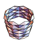
Figure 1. A discrete PS surface of revolution with the parameters $q=0.8$ and $c=\pi/8$. The right figure is a wired model of the left one. The figures are made by using Wolfram Mathematica 10.

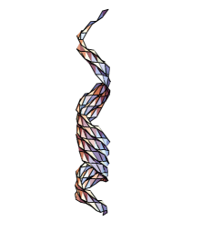
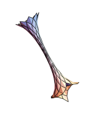
Figure 2. (Left) a discrete PS surface is given by the same data in Figure 1 and the spectral parameter has been chosen as $\lambda=1.5$ in Sym formula (2.6). The surface has a screw motion symmetry. (Right) a discrete PS surface of revolution with the parameters $q=0.4$ and $c=\pi/8$.

Appendix

In this appendix we give a definition of the loop group of ${\rm SU}_{2}$ and its subgroups $\Lambda^{\pm}{\rm SU}_{2}$. Moreover theorem of the Birkhoff decomposition will be stated.

It is easy to see that $F$ defined in (2.3) together with the condition $F|_{(x_{*},y_{*})}=\operatorname{Id}$ is an element in the twisted ${\rm SU}_{2}$-loop group:

(3.2) $$\Lambda{\rm SU}_{2}:=\left\{g:\mathbb{R}^{\times}\cup S^{1}\to{\rm SL}_{2}\mathbb{C}\;\Big{|}\;\begin{array}[]{l}\mbox{ $g$ is smooth, $g(\lambda)=\left(\overline{g(\bar{\lambda})}^{-1}\right)^{T}$}\\ \mbox{\;and $\sigma g(\lambda)=g(-\lambda)$}\end{array}\right\},$$

where $\mathbb{R}^{\times}=\mathbb{R}\setminus\{0\}$, $\sigma X=\operatorname{Ad}(\sigma_{3})X=\sigma_{3}X\sigma_{3}^{-1},(X\in{\rm SL}_{2}\mathbb{C})$ is an involution on ${\rm SL}_{2}\mathbb{C}$. In order to make the above group a Banach Lie group, we restrict the occurring matrix coefficients to the Wiener algebra $\mathcal{A}=\{f(\lambda)=\sum_{n\in\mathbb{Z}}f_{n}\lambda^{n}:S^{1}\rightarrow\mathbb{C}\;|\;\sum_{n\in\mathbb{Z}}|f_{n}|<\infty\}$, where we denote the Fourier expansion of $f$ on $S^{1}$ by $f(\lambda)=\sum_{n\in\mathbb{Z}}f_{n}\lambda^{n}$. Then the Wiener algebra is a Banach algebra relative to the norm $\|f\|=\sum|f_{n}|$ and the loop group $\Lambda{\rm SU}_{2}$ is a Banach Lie group, [6].

Let $\mathbb{D}^{+}$ and $\mathbb{D}^{-}$ be the interior of the unit disk in the complex plane and the union of the exterior of the unit disk in the complex plane and infinity, respectively. We first define two subgroups of $\Lambda{\rm SU}_{2}$:

(3.3) $$\Lambda^{+}{\rm SU}_{2}=\left\{g\in\Lambda{\rm SU}_{2}\;|\;\mbox{$g$ can be analytically extended to $\mathbb{D}^{+}$}\right\},$$

(3.4) $$\Lambda^{-}{\rm SU}_{2}=\left\{g\in\Lambda{\rm SU}_{2}\;|\;\mbox{$g$ can analytically be extended to $\mathbb{D}^{-}$}\right\}.$$

Then $\Lambda^{+}_{*}{\rm SU}_{2}$ and $\Lambda^{-}_{*}{\rm SU}_{2}$ denote subgroups of $\Lambda^{+}{\rm SU}_{2}$ and $\Lambda^{-}{\rm SU}_{2}$ normalized at $\lambda=0$ and $\lambda=\infty$, respectively:

$$\Lambda^{+}_{*}{\rm SU}_{2}=\left\{g\in\Lambda^{+}{\rm SU}_{2}\;|\;g(\lambda=0)=\operatorname{Id}\right\},$$

$$\Lambda^{-}_{*}{\rm SU}_{2}=\left\{g\in\Lambda^{-}{\rm SU}_{2}\;|\;g(\lambda=\infty)=\operatorname{Id}\right\}.$$

The following decomposition theorem is fundamental.

Theorem 3.3 (Birkhoff decomposition, [6, 3]).

The multiplication maps

$$\Lambda^{+}_{*}{\rm SU}_{2}\times\Lambda^{-}{\rm SU}_{2}\to\Lambda{\rm SU}_{2}\;\;\mbox{and}\;\;\Lambda^{-}_{*}{\rm SU}_{2}\times\Lambda^{+}{\rm SU}_{2}\to\Lambda{\rm SU}_{2}$$

are diffeomorphisms onto $\Lambda{\rm SU}_{2}$, respectively.

References

• [1] A. Bobenko and U. Pinkall. Discrete surfaces with constant negative Gaussian curvature and the Hirota equation. J. Differential Geom., 43, no. 3, 527 – 611, 1996.
• [2] A. Bobenko and U. Pinkall. Discretization of surfaces and integrable systems. Discrete integrable geometry and physics (Vienna, 1996). Oxford Lecture Ser. Math. Appl., 16, 3 – 58, 1999.
• [3] D. Brander. Loop group decompositions in almost split real forms and applications to soliton theory and geometry. J. Geom. Phys. 58, no. 12, 1792 – 1800, 2008.
• [4] D. Brander, J. Inoguchi, S.-P. Kobayashi. Constant Gaussian curvature surfaces in the 3-sphere via loop groups. Pacific J. Math., 269, no. 2, 281 – 303, 2014.
• [5] J. F. Dorfmeister, T. Ivey and I. Sterling. Symmetric pseudospherical surfaces. I. General theory. Results Math., 56, no. 1 – 4, 3–21, 2009.
• [6] I. Ts. Gohberg. The factorization problem in normed rings, functions of isometric and symmetric operators, and singular integral equations. Russian Math. Surv., 19, 63 – 114, 1964.
• [7] R. Hirota. Nonlinear partial difference equations. III. Discrete sine-Gordon equation. J. Phys. Soc. Japan, 43, no. 6, 2079 – 2086, 1977.
• [8] J. Inoguchi, K. Kajiwara, N. Matsuura and Y. Ohta. Discrete mKdV and discrete sine-Gordon flows on discrete space curves. J. Phys. A, 47, no.23, 235022, 26pp, 2014.
• [9] S.-P. Kobayashi. Nonlinear d’Alembert formula for discrete pseudospherical surfaces. Preprint, arXiv:1505.07189, 2015.
• [10] I. M. Kričever. An analogue of the d’Alembert formula for the equations of a principal chiral field and the sine-Gordon equation. Dokl. Akad. Nauk SSSR, 253, no. 2, 288 – 292, 1980.
• [11] M. Melko and I. Sterling. Application of soliton theory to the construction of pseudospherical surfaces in ${\bf R}^{3}$. Ann. Global Anal. Geom., 11, no. 1, 65 – 107, 1993.
• [12] A. Sym. Soliton surfaces and their applications (soliton geometry from spectral problems). Geometric aspects of the Einstein equations and integrable systems (Scheveningen, 1984), Lecture Notes in Phys., 239, 154 – 231, 1985.
• [13] M. Toda. Weierstrass-type representation of weakly regular pseudospherical surfaces in Euclidean space. Balkan J. Geom. Appl., 7, no. 2, 87 – 136, 2002.