Study of Distributed Spectrum Estimation Using Alternating Mixed Discrete-Continuous Adaptation

Abstract

This paper proposes a distributed alternating mixed discrete-continuous (DAMDC) algorithm to approach the oracle algorithm based on the diffusion strategy for parameter and spectrum estimation over sensor networks. A least mean squares (LMS) type algorithm that obtains the oracle matrix adaptively is developed and compared with the existing sparsity-aware and conventional algorithms. The proposed algorithm exhibits improved performance in terms of mean square deviation and power spectrum estimation accuracy. Numerical results show that the DAMDC algorithm achieves excellent performance.

I Introduction

Distributed signal processing strategies are very promising tools for solving parameter estimation problems in wireless networks and applications such as sensor networks [1, 2, 3]. These techniques can exploit the spatial diversity available in a network of sensors to obtain increased estimation accuracy and robustness against sensor failures.

Another set of tools for enhancing the performance of signal processing algorithms is the exploitation of sparsity, work on which initially dealt with centralized problems [4, 5, 6, 7, 8, 9, 10, 11, 12, 13, 16, 14, 15] and, more recently, has examined distributed techniques [17, 18, 19, 20, 22, 23, 24, 25, 26, 27] in several applications. A common strategy among the techniques reported so far is the development of adaptive algorithms such as the least mean squares (LMS) [8, 16, 18, 19, 20, 22, 25, 26] and recursive least-squares (RLS) [11, 12, 23, 26] using different penalty functions. Such penalty functions perform a regularization that attracts to zero the elements of the parameter vector with small magnitudes. The most well-known and successful penalty functions are the $l_{0}$-norm [5, 11], the $l_{1}$-norm [8] and the log-sum penalty [4, 8]. The optimal algorithm for processing sparse signals is known as the oracle algorithm [16], which requires an exhaustive search for the location of the non-zero coefficients followed by parameter estimation.

With the development and increasing deployment of mobile networks, the frequency spectrum has become a resource that should be exploited in a judicious way to avoid interference. By estimating the power spectrum with spatially distributed sensors this resource can be planned and properly exploited [18, 19, 21]. Diffusion adaptation strategies incorporating sparsity constraints have been used to solve distributed spectrum estimation problems in [18] and [19]. However, prior work on distributed techniques that approach the oracle algorithm is rather limited, and adaptive techniques that exploit potential sparsity of signals using discrete and continuous variables have not been developed so far.

In this work, we propose a sparsity-aware distributed alternating mixed discrete-continuous LMS (DAMDC-LMS) algorithm based on the diffusion adapt-then-combine (ATC) protocol. We consider an alternating optimization strategy with an LMS-type recursion along with a mapping from continuous to discrete variables, which is used to find the actual non-zero values, and another LMS-type recursion that performs continuous adaptation. In particular, the proposed DAMDC-LMS algorithm is incorporated into a distributed spectrum estimation strategy. DAMDC-LMS is compared with prior art in a distributed spectrum estimation application.

This paper is organized as follows. Section II describes the system model and the problem statement. Section III presents the proposed DAMDC-LMS algorithm. Section IV details the proposed algorithm for an application to spectrum estimation. Section V presents and discusses the simulation results. Finally, Section VI provides our conclusions.

Notation: In this paper, matrices and vectors are designated by boldface upper case letters and boldface lower case letters, respectively. The superscript $(.)^{H}$ denotes the Hermitian operator, $\|.\|^{1}$ refers to the $l_{1}$-norm and $E[\cdot]$ denotes expected value.

II System Model and Problem Statement

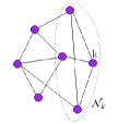
Figure 1: Network topology with $N$ nodes.

We consider a network that is partially connected and consists of $N$ nodes that exchange information among themselves. Each node $k$ employs a parameter estimator and has its neighborhood described by the set ${\mathcal{N}}_{k}$, as shown in Fig. 1. The task of parameter estimation is to adjust an M $\times 1$ weight vector $\boldsymbol{\omega}_{k,i}$ at each node $k$ and time $i$ based on an M$\times 1$ input signal vector $\boldsymbol{x}_{k,i}$ and ultimately estimate an unknown M $\times 1$ system parameter vector $\boldsymbol{\omega}_{0}$ [1]. The desired signal $d_{k,i}$ at each time $i$ and node $k$ is drawn from a random process and given by

$$\ d_{k,i}=\boldsymbol{\omega}_{0}^{H}\boldsymbol{x}_{k,i}+n_{k,i},$$ (1)

where $n_{k,i}$ is measurement noise.

We consider a distributed estimation problem for a network in which each agent $k$ has access at each time instant to a realization of zero-mean spatial data $\{d_{k,i},\boldsymbol{x}_{k,i}\}$ [1, 3]. The goal of the network is to minimize the following cost function:

$$\begin{split}C(\boldsymbol{\omega}_{k,i})&=\sum_{k=1}^{N}E[|d_{k,i}-\hat{d}_{k,i}|^{2}]\\ &=\sum_{k=1}^{N}E[|d_{k,i}-\boldsymbol{\omega}_{k,i}^{H}\boldsymbol{x}_{k,i}|^{2}],~{}{\rm for}~{}k=1,2,\ldots,N,\end{split}$$ (2)

By solving this minimization problem one can obtain the optimum solution for the weight vector at each node. For a network with possibly sparse parameter vectors, the cost function might also involve a penalty function that exploits sparsity. In what follows, we present a novel distributed diffusion technique to approach the oracle algorithm and efficiently solve (2) under sparseness conditions.

III Proposed DAMDC-LMS Algorithm

In this section, we detail the proposed distributed scheme and DAMDC-LMS algorithm using the diffusion ATC strategy. The proposed scheme for each agent $k$ of the network is shown in Fig. 2. The output estimate of the proposed scheme is given by

$$\begin{split}\hat{d}_{k,i}&=\boldsymbol{\omega}_{k,i}^{H}\boldsymbol{P}_{k,i}\boldsymbol{x}_{k,i}=\boldsymbol{p}^{T}_{k,i}\boldsymbol{W}^{*}_{k,i}\boldsymbol{x}_{k,i}\\ &=\boldsymbol{x}^{T}_{k,i}\boldsymbol{W}^{*}_{k,i}\boldsymbol{p}_{k,i}=\boldsymbol{x}^{T}_{k,i}\boldsymbol{P}_{k,i}\boldsymbol{\omega}^{*}_{k,i},\end{split}$$ (3)

where the parameter vector ${\boldsymbol{\omega}}_{k,i}$ is a column vector of $M$ coefficients related to the diagonal matrix $\boldsymbol{W}_{k,i}={\rm diag}(\boldsymbol{\omega}_{k,i})$. The matrix $\boldsymbol{P}_{k,i}$ is a square diagonal matrix with $M$ elements that is applied to the input vector $\boldsymbol{x}_{k,i}$ and aims to simulate the oracle algorithm by identifying the null positions of $\boldsymbol{\omega}_{0}$.

In order to obtain recursions for ${\boldsymbol{P}}_{k,i}$ and ${\boldsymbol{\omega}}_{k,i}$ we compute the stochastic gradient of the cost function in (2) with respect to both parameters, where the optimization of ${\boldsymbol{P}}_{k,i}$ involves discrete variables and ${\boldsymbol{\omega}}_{k,i}$ deals with continuous variables. In particular, we develop an alternating optimization approach using an LMS type algorithm that consists of a recursion for ${\boldsymbol{P}}_{k,i}$ and another recursion for ${\boldsymbol{\omega}}_{k,i}$ that are employed in an alternating fashion.

Figure 2: Proposed adaptive scheme at node $k$.

In order to compute ${\boldsymbol{P}}_{k,i}$ and ${\boldsymbol{\omega}}_{k,i}$ we must solve the mixed discrete-continuous non-convex optimization problem:

$$\begin{split}{\boldsymbol{p}}_{k,i}^{*},{\boldsymbol{\omega}}_{k,i}^{*}&=\min_{{\boldsymbol{p}}_{k,i}\in{\mathcal{I}}^{M\times 1},~{}~{}{\boldsymbol{\omega}}_{k,i}\in{\mathcal{C}}^{M\times 1}}C({\boldsymbol{p}}_{k,i},{\boldsymbol{\omega}}_{k,i}),\\ &~{}{\rm for}~{}k=1,2,\ldots,N,\end{split}$$ (4)

where

$$C({\boldsymbol{p}}_{k,i},{\boldsymbol{\omega}}_{k,i})=\sum_{k=1}^{N}E[|d_{k,i}-\boldsymbol{p}^{T}_{k,i}{\boldsymbol{W}}^{H}_{k,i}{\boldsymbol{x}}_{k,i}|^{2}],$$ (5)

${\boldsymbol{p}}_{k,i}$ contains the elements of the main diagonal of ${\bf P}_{k,i}$, and ${\mathcal{I}}^{M\times 1}$ denotes the set of $M$-dimensional binary vectors with values $0$ and $1$. Since the problem in (4) is NP-hard, we resort to an approach that assumes ${\boldsymbol{p}}_{k,i}$ is a real-valued continuous parameter vector for its computation and then map ${\boldsymbol{p}}_{k,i}$ to discrete values. The relations in (3) allow us to compute the gradient of the cost function with respect to ${\boldsymbol{p}}_{k,i}$ and ${\boldsymbol{\omega}}_{k,i}$ and their diagonal versions ${\boldsymbol{P}}_{k,i}$ and ${\boldsymbol{W}}^{H}_{k,i}$, respectively. The gradient of the cost function with respect to ${\boldsymbol{p}}_{k,i}$ is given by

$$\begin{split}\nabla_{\boldsymbol{p}_{k,i}}C(\boldsymbol{p}_{k,i},\boldsymbol{\omega}_{k,i})&=\frac{\partial}{\partial\boldsymbol{p}_{k,i}}\Big{(}E|d_{k,i}|^{2}-(\boldsymbol{p}^{T}_{k,i}\boldsymbol{W}^{*}_{k,i}E[d^{*}_{k,i}\boldsymbol{x}_{k,i}])\\ &\quad+\boldsymbol{p}^{T}_{k,i}\boldsymbol{W}^{*}_{k,i}E[\boldsymbol{x}_{k,i}\boldsymbol{x}^{H}_{k,i}\boldsymbol{W}_{k,i}\boldsymbol{p}_{k,i}]\\ &\quad-E[d_{k,i}\boldsymbol{x}^{H}_{k,i}]\boldsymbol{W}_{k,i}\boldsymbol{p}_{k,i}\Big{)}.\end{split}$$ (6)

Replacing the expected values with instantaneous values, we obtain

$$\begin{split}\hat{\nabla}_{\boldsymbol{p}_{k,i}}C(\boldsymbol{p}_{k,i},\boldsymbol{\omega}_{k,i})&=\frac{\partial}{\partial\boldsymbol{p}_{k,i}}\Big{(}|d_{k,i}|^{2}-\boldsymbol{p}^{T}_{k,i}\boldsymbol{W}^{*}_{k,i}d^{*}_{k,i}\boldsymbol{x}_{k,i}\\ &\quad+\boldsymbol{p}^{T}_{k,i}\boldsymbol{W}^{*}_{k,i}\boldsymbol{x}_{k,i}\boldsymbol{x}^{H}_{k,i}\boldsymbol{W}_{k,i}\boldsymbol{p}_{k,i}\\ &\quad-d_{k,i}\boldsymbol{x}^{H}_{k,i}\boldsymbol{W}_{k,i}\boldsymbol{p}_{k,i}\Big{)}.\end{split}$$ (7)

Computing the gradient of the cost function with respect to ${\boldsymbol{p}}_{k,i}$, we obtain

$$\begin{split}\hat{\nabla}_{\boldsymbol{p}_{k,i}}C(\boldsymbol{p}_{k,i},\boldsymbol{\omega}_{k,i})&=d^{*}_{k,i}\boldsymbol{W}^{*}_{k,i}{\boldsymbol{x}}_{k,i}-d_{k,i}\boldsymbol{W}^{T}_{k,i}\boldsymbol{x}^{*}_{k,i}\\ &\quad+\boldsymbol{W}^{*}_{k,i}\boldsymbol{x}_{k,i}\boldsymbol{x}^{H}_{k,i}\boldsymbol{W}_{k,i}\boldsymbol{p}_{k,i}\\ &\quad+\boldsymbol{W}^{T}_{k,i}\boldsymbol{x}^{*}_{k,i}\boldsymbol{x}^{T}_{k,i}\boldsymbol{W}^{H}_{k,i}\boldsymbol{p}_{k,i}.\end{split}$$ (8)

Grouping common terms, we arrive at

$$\begin{split}\hat{\nabla}_{\boldsymbol{p}_{k,i}}C(\boldsymbol{p}_{k,i},\boldsymbol{\omega}_{k,i})&=-\Big{(}d_{k,i}-\boldsymbol{x}^{H}_{k,i}\boldsymbol{W}_{k,i}\boldsymbol{p}_{k,i}\boldsymbol{W}_{k,i}\boldsymbol{x}_{k,i}\\ &\quad+d_{k,i}-\boldsymbol{x}^{T}_{k,i}\boldsymbol{W}^{H}_{k,i}\boldsymbol{p}_{k,i}\boldsymbol{W}^{T}_{k,i}\boldsymbol{x}^{*}_{k,i}\Big{)},\end{split}$$ (9)

where $\boldsymbol{p}_{k,i}$ is a real parameter vector, $\boldsymbol{p}_{k,i}=\boldsymbol{p}^{*}_{k,i}$, $\boldsymbol{p}^{H}_{k,i}=[\boldsymbol{p}^{*}_{k,i}]^{T}=\boldsymbol{p}^{T}_{k,i}$. Since $\boldsymbol{W}_{k,i}$ is symmetric, i.e., $\boldsymbol{W}^{T}_{k,i}=\boldsymbol{W}_{k,i}$, we have $\boldsymbol{W}^{H}_{k,i}=[\boldsymbol{W}^{*}_{k,i}]^{T}=[\boldsymbol{W}^{T}_{k,i}]^{*}=\boldsymbol{W}^{*}_{k,i}$. The terms in (9) represent the sum of a vector and its conjugate:

$$\begin{split}\hat{\nabla}_{\boldsymbol{p}_{k,i}}C(\boldsymbol{p}_{k,i},\boldsymbol{\omega}_{k,i})&=-\underbrace{\Big{(}\big{(}d_{k,i}-\boldsymbol{x}^{H}_{k,i}\boldsymbol{W}_{k,i}\boldsymbol{p}_{k,i}\big{)}\boldsymbol{W}^{*}_{k,i}\boldsymbol{x}_{k,i}}_{A}\\ &\quad+\underbrace{\big{(}d_{k,i}-\boldsymbol{x}^{T}_{k,i}\boldsymbol{W}^{H}_{k,i}\boldsymbol{p}_{k,i}\big{)}\boldsymbol{W}_{k,i}\boldsymbol{x}^{*}_{k,i}\Big{)}}_{A^{*}}.\end{split}$$ (10)

Applying the property $A+A^{*}=2\Re(A)$, we have

$$\hat{\nabla}_{\boldsymbol{p}_{k,i}}\mbox{MSE}(\boldsymbol{p}_{k,i},\boldsymbol{\omega}_{k,i})=2\Re(A).$$ (11)

The recursion to update the parameter vector ${\boldsymbol{p}}_{k,i}$ is given by

$$\begin{split}\boldsymbol{p}_{k,i+1}&=\boldsymbol{p}_{k,i}-\eta\hat{\nabla}_{\boldsymbol{p}_{k,i}}\mbox{MSE}(\boldsymbol{p}_{k,i},\boldsymbol{W}_{k,i})\\ &=\boldsymbol{p}_{k,i}+2\eta\Re(e_{p_{k,i}}^{*}\boldsymbol{x}^{H}_{k,i}\boldsymbol{W}_{k,i}),\end{split}$$ (12)

where the error signal is given by

$$\ e_{p_{k,i}}=d_{k,i}-\boldsymbol{p}^{T}_{k,i}\boldsymbol{W}_{i-1}\boldsymbol{x}_{k,i}.$$ (13)

For the update of the parameter vector ${\boldsymbol{w}}_{k,i}$, we can apply well-known adaptive algorithms. By computing the gradient of the cost function with respect to ${\boldsymbol{w}}_{k,i}^{*}$, we have

$$\nabla C_{{\boldsymbol{w}}^{*}_{k,i}}({\boldsymbol{p}}_{k,i},{\boldsymbol{w}}_{k,i})=(d_{k,i}-\boldsymbol{x}^{T}_{k,i}{\boldsymbol{P}}_{k,i}\boldsymbol{\omega}^{*}_{i-1})^{*}{\boldsymbol{P}}_{k,i}{\boldsymbol{x}}_{k,i}$$ (14)

The following LMS type recursion updates the parameter vector ${\boldsymbol{\omega}}_{k,i}$:

$$\boldsymbol{\omega}_{k,i+1}=\boldsymbol{\omega}_{k,i}+\mu e^{*}_{k,i}\boldsymbol{P}_{k,i}\boldsymbol{x}_{k,i},$$ (15)

where the error signal is given by $e_{k,i}=d_{k,i}-\boldsymbol{x}^{T}_{k,i}\boldsymbol{P}_{k,i}\boldsymbol{\omega}^{*}_{i-1}$.

The recursions for ${\boldsymbol{p}}_{k,i}$ and ${\boldsymbol{\omega}}_{k,i}$ using the ATC protocol [1, 2] for $k=1,2,\ldots,N$ are then given by

$$\boldsymbol{p}_{k,i+1}=\boldsymbol{p}_{k,i}+2\eta\Re(e_{p_{k,i}}^{*}\boldsymbol{x}_{k,i}^{H}\boldsymbol{W}_{k,i}),$$ (16)

$$\boldsymbol{\varphi}_{k,i+1}=\boldsymbol{\omega}_{k,i-1}+\mu e^{*}_{k,i}\boldsymbol{P}_{k,i}\boldsymbol{x}_{k,i},\\$$ (17)

$$\boldsymbol{\omega}_{k,i}=\sum_{l\in N_{k}}a_{lk}\boldsymbol{\varphi}_{l,i},$$ (18)

where (16) and (17) are the adaptation step, and (18) is the combination step of the ATC protocol. The combining coefficients of the latter are represented by $a_{lk}$ and should comply with

$$\sum_{l\in N_{k}}a_{lk}=1,\ l\in N_{k,i},\forall k.$$ (19)

The strategy adopted in this work for the $a_{lk}$ combiner is the Metropolis rule [1] given by

$$a_{kl}=\left\{\begin{array}[]{ll}\frac{1}{max\{|\mathcal{N}_{k}|,|\mathcal{N}_{l}|\}}\ \ $if\ $k\neq l$\ are linked$,\\ 1-\sum\limits_{l\in\mathcal{N}_{k}/k}a_{kl},\ \ $for\ $k$\ =\ $l$$.\end{array}\right.$$ (20)

In order to compute the discrete vector $\boldsymbol{p}_{k,i}$, we rely on a simple approach that maps the continuous variables into discrete variables, which is inspired by the likelihood ascent approach adopted for detection problems in wireless communications [28, 29]. The initial value at each node is an all-one vector ($\boldsymbol{p}_{k,0}=\boldsymbol{1}$ or $\boldsymbol{P}_{k,0}=\boldsymbol{I}$). The $\boldsymbol{\omega}_{k,i}$ vector is initialized as an all-zero vector ($\boldsymbol{\omega}_{k,0}=\boldsymbol{0}$ or $\boldsymbol{W}_{k,0}=\boldsymbol{0}$). After each iteration of (16), we obtain discrete values from $\boldsymbol{p}_{k,i}$ using the following rule for $m=1,\ldots,M$:

$$p_{k,i+1}^{m}=\left\{\begin{array}[]{ll}1,\ $if\ $p_{k,i}^{m}>\tau,\\ 0,\ \mbox{otherwise},\end{array}\right.$$ (21)

where $\tau$ is a threshold used to determine the positions of the non-zero values of the parameter vector $\boldsymbol{p}_{k,i}$. The goal is to approach the results of the oracle algorithm and an appropriate value for $\tau$ can be obtained experimentally.

IV Distributed Spectrum Estimation using the DAMDC-LMS Algorithm

We now illustrate the use of DAMDC-LMS in distributed spectrum estimation, which aims to estimate the spectrum of a transmitted signal $s$ with $N$ nodes using a wireless sensor network [3, 18, 19]. The power spectral density (PSD) of the signal $s$ at each frequency denoted by $\Phi_{s}(f)$ is given by

$$\ \Phi_{s}(f)=\sum_{m=1}^{M}b_{m}(f)\omega_{0m}=\boldsymbol{b}_{0}^{T}(f)\boldsymbol{\omega}_{0},$$ (22)

where $\boldsymbol{b}_{0}(f)=[b_{1}(f),...,b_{M}(f)]^{T}$ is the vector of basis functions evaluated at frequency $f$, $\boldsymbol{\omega}_{0}=[\omega_{01},...,\omega_{0M}]$ is a vector of weighting coefficients representing the transmit power of the signal $s$ over each basis, and $M$ is the number of basis functions. For $M$ sufficiently large, the basis expansion in (22) can approximate well the spectrum. Possible choices for the set of basis functions $\{{b_{m}(f)\}}_{m=1}^{M}$ include rectangular functions, raised cosines, Gaussian bells and splines [27].

We denote the channel transfer function between a transmit node conveying the signal $s$ and receive node $k$ at time instant $i$ by $H_{k}(f,i)$, and thus the PSD of the received signal observed by node k can be expressed as

$$\begin{split}\Phi_{k}(f,i)&=|H_{k}(f,i)|^{2}\Phi_{s}(f)+\upsilon^{2}_{n,k},\\ &=\sum_{m=1}^{M}|H_{k}(f,i)|^{2}b_{m}(f)\omega_{0m}+\upsilon^{2}_{n,k},\\ &=\boldsymbol{b}_{k,i}^{T}(f)\boldsymbol{\omega}_{0m}+\upsilon^{2}_{n,k}.\end{split}$$ (23)

where $\boldsymbol{b}_{k,i}^{T}(f)=[|H_{k}(f,i)|^{2}b_{m}(f)]^{M}_{m=1}$ and $\upsilon_{n,k}^{2}$ is the noise power of the receiver at node $k$.

Following the distributed model, at every iteration $i$ every node $k$ measures the PSD $\Phi_{k}(f,i)$ presented in (23) over $N_{c}$ frequency samples $f_{j}=f_{min}:(f_{max}-f_{min})/N_{c}:f_{max}$, for $j=1,...,N_{c}$, the desired signal is given by

$$\ d_{k,i}(j)=\boldsymbol{b}_{k,i}^{T}(f_{j})\boldsymbol{\omega}_{0}+\upsilon_{n,k}^{2}+n_{k,i}(j),$$ (24)

where the last term denotes the observation noise with zero mean and variance $\sigma_{n,j}^{2}$. The noise power $\upsilon_{n,k}^{2}$ at the receiver of node $k$ can be estimated with high accuracy in a preliminary step using, e.g., an energy estimator over an idle band, and then subtracted from (24). A linear model is obtained from the measurements over $N_{c}$ contiguous channels

$$\ \boldsymbol{d}_{k,i}=\boldsymbol{B}_{k,i}\boldsymbol{\omega}_{0}+\boldsymbol{n}_{k,i},$$ (25)

where $\boldsymbol{B}_{k,i}=[\boldsymbol{b}_{k,i}^{T}(f_{j})]_{j=1}^{N_{c}}\in{\mathcal{R}}^{N_{c}\times M}$, and $\boldsymbol{n}_{k,i}$ is a zero mean random vector. Then we can introduce the cost function for each agent $k$ described by

$$\ C(\boldsymbol{\omega}_{k,i})=E[|\boldsymbol{d}_{k,i}-\boldsymbol{B}_{k,i}\boldsymbol{\omega}_{k,i}|^{2}],~{}{\rm for}~{}k=1,\ldots,N.$$ (26)

Once we have the cost function, the DAMDC-LMS algorithm can be applied by introducing the discrete parameter vector $\boldsymbol{p}_{k,i}$ in (26), which results in

$$\ C(\boldsymbol{\omega}_{k,i},\boldsymbol{p}_{k,i})=E[|\boldsymbol{d}_{k,i}-\boldsymbol{B}_{k,i}\boldsymbol{P}_{k,i}\boldsymbol{\omega}_{k,i}|^{2}],~{}{\rm for}~{}k=1,\ldots,N,$$ (27)

where $\boldsymbol{P}_{k,i}$ is the $B\times B$ diagonal matrix to exploit the sparsity for a more accurate spectrum estimation. Introducing the matrix $\boldsymbol{P}_{k,i}$ for exploiting sparsity in the recursions (16), (17) and (18), we obtain for $k=1,2,\ldots,N$:

$${\rm Adaptation}\left\{\begin{array}[]{ll}\boldsymbol{p}_{k,i+1}=\boldsymbol{p}_{k,i}+2\eta\Re(e_{p_{k,i}}^{*}\boldsymbol{B}_{k,i}^{H}\boldsymbol{W}_{k,i-1})\\ p_{k,i+1}^{m}=\left\{\begin{array}[]{ll}1,\ $if\ $p_{k,i}^{m}>\tau,~{}{\rm for}~{}m=1,\ldots,M,\\ 0,\ \mbox{otherwise},\end{array}\right.\\ \boldsymbol{\varphi}_{k,i+1}=\boldsymbol{\omega}_{k,i-1}+\mu e^{*}_{k,i}\boldsymbol{P}_{k,i}\boldsymbol{B}_{k,i},\\ \end{array}\right.$$ (28)

$${\rm Combination}\left\{\begin{array}[]{ll}\boldsymbol{\omega}_{k,i}=\sum_{l\in N_{k}}a_{lk}\boldsymbol{P}_{k,i}\boldsymbol{\varphi}_{l,i}.\end{array}\right.$$ (29)

The positions in $\boldsymbol{p}_{k,i}$ with ones indicate the information content at each node and sample of the signal. With this approach, we can identify the positions of the non-zero coefficients of the frequency spectrum and achieve performance similar to that of the oracle algorithm as seen in the following section.

V Simulation Results

In this section, we evaluate the performance of the DAMDC-LMS algorithm for distributed spectrum estimation using sensor networks, where DAMDC-LMS is compared with existing algorithms. The results are shown in terms of the mean square deviation (MSD), power and PSD estimation.

We consider a network with $20$ nodes for estimating the unknown spectrum $\boldsymbol{\omega}_{0}$ and set the threshold to $\tau=1$, which according to our studies obtained the best performance for the scenarios under evaluation. Each iteration corresponds to a time instant. The results are averaged over 100 experiments. The nodes scan $100$ frequencies over the frequency axis, which is normalized between $0$ and $1$, and use $B=50$ non$-$overlapping rectangular basis functions to model the expansion of the spectrum [24]. The basis functions have amplitudes equal to one. We assume that the unknown spectrum $\boldsymbol{\omega}_{0}$ is examined over 8 basis functions, leading to a sparsity ratio equal to $S=8/50$. The power transmitted over each basis function is set to $0.7$ mW and noise variance is set to $0.001$. For distributed spectrum estimation, we have compared the proposed DADMC-LMS algorithm, the oracle ATC-LMS, the RZA-ATC-LMS [18], the $l_{0}$-ATC-LMS [18] and the standard ATC-LMS algorithms with the parameters optimized. We first measure the performance of the algorithms in terms of MSD as shown in Fig. 3. The results show that DAMDC-LMS outperforms standard and sparsity-aware algorithms and exhibits performance close to that of the oracle algorithm, provided that the step sizes are appropriately adjusted.

Figure 3: MSD for distributed spectrum estimation. Parameters: $\mu=0.05$, $\eta=5\times 10^{-2}$ , $\rho_{\rm RZA}=3.5\times 10^{-5}$, $\rho_{l_{0}}=3.5\times 10^{-5}$, $\rho_{ACS}=10^{-3}$, $\beta=5$, $\beta_{A}CS=50$, $\epsilon=0.1$, ${\rm SNR}=30dB$, $\tau=1$ and $S=8/50$.

In a second example, we assess the PSD estimation performance of the algorithms. Fig. 4 shows that the DAMDC-LMS algorithm is able to accurately estimate the spectrum consistently with the oracle algorithm.

Figure 4: Distributed spectrum estimation. Parameters: $\mu=0.45$, $\eta=0.5\times 10^{-3}$ ,$\rho_{l_{0}}=3\times 10^{-5}$, $\tau=1$, $\beta=50$ and $S=8/50$.

In order to verify the adaptation performance of DAMDC-LMS, in Fig. 5 we evaluate the behavior of the PSD estimates over an initially busy channel (the $16$-th channel in this case) that ceases to be busy after $500$ iterations, by comparing the results achieved by the DAMDC-LMS and the oracle algorithms. We consider the same settings of the previous example. The transmit power is set to $0.20$ mW. We notice that DADMC-LMS is able to more effectively track the spectrum as compared to the oracle algorithm due to its rapid learning.

Figure 5: Power spectrum tracking. Parameters: $\mu=0.45$, $\eta=0.5\times 10^{-3}$ ,$\rho_{l_{0}}=3\times 10^{-5}$, $\beta=50$, $\tau=1$ and $S=8/50$.

VI Conclusion

In this work, we have proposed a distributed sparsity-aware algorithm for spectrum estimation over sensor networks. The proposed DADMC-LMS algorithm outperforms previously reported algorithms. Simulations have shown that DADMC-LMS can obtain lower MSD values and faster convergence than prior art and close to that of the oracle algorithm.

References

• [1] C. G. Lopes and A. H. Sayed, β€œDiffusion least-mean squares over adaptive networks: Formulation and performance analysis,” IEEE Transactions on Signal Processing, vol. 56, no. 7, pp. 3122-3136, July 2008.
• [2] F. S. Cattivelli and A. H. Sayed, β€œDiffusion LMS strategies for distributed estimation,” IEEE Transactions on Signal Processing, vol. 58, pp. 1035-1048, March 2010.
• [3] G. Mateos, J. A. Bazerque, and G. B. Giannakis, β€œDistributed sparse linear regression,” IEEE Transactions on Signal Processing, vol. 58, no. 10, pp. 5262-5276, Oct 2010.
• [4] E. J. Candes, M. Wakin, and S. Boyd, β€œEnhancing sparsity by reweighted l1 minimization,” Journal of Fourier Analysis and Applications, 2008.
• [5] Y. Gu, J. Jin, and S. Mei, β€œL0subscript𝐿0L_{0}-norm constraint LMS algorithm for sparse system identification,” IEEE Signal Processing Letters, vol. 16, pp. 774-777, 2009.
• [6] R. C. de Lamare and R. Sampaio-Neto, β€œAdaptive reduced-rank MMSE filtering with interpolated FIR filters and adaptive interpolators”, IEEE Sig. Proc. Letters, vol. 12, no. 3, 2005, pp. 177 - 180.
• [7] R. C. de Lamare and R. Sampaio-Neto, β€œReduced-rank adaptive filtering based on joint iterative optimization of adaptive filters”, IEEE Signal Process. Lett., vol. 14, no. 12, pp. 980-983, Dec. 2007.
• [8] Y. Chen, Y. Gu, and A. O. Hero, β€œSparse LMS for system identification,” Proc. IEEE International Conference on Acoustics, Speech and Signal Processing (ICASSP), April 2009.
• [9] R. C. de Lamare and R. Sampaio-Neto, β€œAdaptive Reduced-Rank Processing Based on Joint and Iterative Interpolation, Decimation and Filtering”, IEEE Transactions on Signal Processing, vol. 57, no. 7, pp. 2503 - 2514, July 2009.
• [10] R. Fa, R. C. de Lamare, and L. Wang, β€œReduced-Rank STAP Schemes for Airborne Radar Based on Switched Joint Interpolation, Decimation and Filtering Algorithm,” IEEE Transactions on Signal Processing, vol.58, no.8, Aug. 2010, pp.4182-4194.
• [11] E. M. Eksioglu and A. L. Tanc, β€œRLS algorithm with convex regularization,” IEEE Signal Processing Letters, vol. 18, no. 8, pp. 470-473, August 2011.
• [12] D. Angelosante, J.A Bazerque, and G.B. Giannakis, β€œOnline adaptive estimation of sparse signals: Where RLS meets the l1-norm,” IEEE Transactions on Signal Processing, vol. 58, no. 7, pp. 3436-3447, July 2010.
• [13] N. Kalouptsidis, G. Mileounis, B. Babadi, and V. Tarokh, β€œAdaptive algorithms for sparse system identification,” Signal Processing, vol. 91, no. 8, pp. 1910-1919, August 2011.
• [14] Z. Yang, R. C. de Lamare and X. Li, β€œL1-Regularized STAP Algorithms With a Generalized Sidelobe Canceler Architecture for Airborne Radar,” IEEE Transactions on Signal Processing, vol.60, no.2, pp.674-686, Feb. 2012.
• [15] Z. Yang, R. C. de Lamare and X. Li, β€œSparsity-aware space-time adaptive processing algorithms with L1-norm regularisation for airborne radar,” IET signal processing, vol. 6, no. 5, pp. 413-423, 2012.
• [16] R. C. de Lamare and R. Sampaio-Neto, β€œSparsity-aware adaptive algorithms based on alternating optimization with shrinkage,” IEEE Signal Processing Letters, vol. 21, no. 2, February 2014.
• [17] S. Chouvardas, K. Slavakis, Y. Kopsinis, and S. Theodoridis, β€œA sparsity promoting adaptive algorithm for distributed learning,” IEEE Transactions on Signal Processing, vol. 60, no. 10, pp. 5412-5425, October 2012.
• [18] P. Di Lorenzo, S. Barbarossa and A. H. Sayed β€œDistributed spectrum estimation for small cell networks based on sparse diffusion adaptation,” IEEE Signal Processing Letters, vol. 20, no. 12, December 2013.
• [19] P. Di Lorenzo and S. Barbarossa, β€œDistributed least-mean squares strategies for sparsity-aware estimation over Gaussian Markov random fields,” Proc. IEEE International Conference on Acoustic, Speech and Signal Processing (ICASSP), May 2014.
• [20] P. Di Lorenzo and A. H. Sayed, β€œSparse distributed learning based on diffusion adaptation,” IEEE Transactions on Signal Processing, vol. 61, no. 6, March 2013.
• [21] P. Di Lorenzo, S. Barbarossa, and Ali H. Sayed, β€œBio-inspired decentralized radio access based on swarming mechanisms over adaptive networks,” IEEE Transactions on Signal Processing, Vol. 61, no. 12, pp. 3183-3197, June 2013.
• [22] R. Arablouei, S. Werner, Y.-F. Huang and K. DoganΓ§ay, β€œDistributed least mean-square estimation with partial diffusion,” IEEE Transactions on Signal Processing, vol. 62, No. 2, pp. 472-484, January 2014.
• [23] Z. Liu, Y. Liu and C. Li, β€œDistributed sparse recursive least-squares over networks,” IEEE Transactions on Signal Processing, vol. 62, no. 6, pp. 1386-1395, March 2014.
• [24] S. Xu and R. C. de Lamare, β€œDistributed conjugate gradient strategies for distributed estimation over sensor networks,” Proc. Sensor Signal Processing for Defense (SSPD), September 2012
• [25] S. Xu, R. C. de Lamare and H. V. Poor, β€œDistributed compressed estimation based on compressive sensing,” IEEE Signal Processing Letters, vol. 22, no. 9, September 2014.
• [26] S. Xu, R. C. de Lamare and H. V. Poor, β€œAdaptive link selection algorithms for distributed estimation,” EURASIP Journal on Advances in Signal Processing, 2015.
• [27] S. Xu, R. C. de Lamare and H. V. Poor, β€œDistributed estimation over sensor networks based on distributed conjugate gradient strategies,” IET Signal Processing, 2016.
• [28] K. Vardhan, S. Mohammed, A. Chockalingam, and B. Rajan, β€œA low-complexity detector for large MIMO systems and multicarrier CDMA systems,” IEEE Journal on Selected Areas in Communications, vol. 26, no. 3, p. 473-485, 2008.
• [29] P. Li and R. C. Murch, β€œMultiple output selection-LAS algorithm in large MIMO systems,” IEEE Communications Letters, vol.14, no.5, pp.399-401, May 2010.
• [30] O. Axelson, Iterative Solution Methods, Cambridge Univ. Press, 1994.
• [31] G. H. Golub and C. F. Van Loan, Matrix Computations, 2nd Ed. Baltimore, MD: Johns Hopkins Univ. Press, 1989.
• [32] S. Theodoridis, Machine Learning: a Bayesian and Optimization Perspective, Academic Press, March 2015.
• [33] N. A. Lynch, Distributed Algorithms, Morgan Kaufmann, 1997.
• [34] O. Jahromi and P. Aarabi, β€œDistributed spectrum estimation in sensor networks,” Proc. IEEE International Conference on Acoustics, Speech, and Signal Processing, vol. 3, pages. 849-52, May 2004.