Ground state properties of quantum Kagomé ice hardcore bosons

Abstract

We study the quantum Kagomé ice hardcore bosons, which corresponds to the XY limit of quantum spin ice Hamiltonian. We estimate the values of the zero-temperature thermodynamic quantities using the large-$S$ expansion. We show that our semi-classical analysis is consistent with finite temperature quantum Monte Carlo estimates.

Keywords: hardcore bosons, condensate fraction, dynamical structure factors.

1 Introduction

The recent search for a putative quantum spin liquid (QSL) state in three-dimensional (3D) pyrochlore lattice quantum spin ice (QSI) has led to a new proposal of quantum spin Hamiltonian devoid of the debilitating quantum Monte Carlo (QMC) sign problem in a wide range of the parameter regime [1, 2, 3]. Recently, Carrasquilla et al. [3], have studied the projected 3D QSI Hamiltonian of Huang, Chen, and Hermele [1] onto a 2D frustrated Kagomé lattice with a [111] crystallographic field. They have explored this model by an explicit finite temperature QMC simulations and identified the interactions that promote a QSL state. In a recent study, we have complemented the QMC analysis using linear spin wave theory [4]. In that study, we found that quantum fluctuations are suppressed in the quantum Kagomé ice model, hence the semiclassical analysis captures a broad trend of the quantum phase diagram and ground state properties uncovered by QMC [3].

However, there remains the possibility of the XY limit of the quantum Kagomé ice (QKI) model. The XY model essentially controls the dynamics of the fully frustrated system, [1, 3] and it forms the basis of ultra-cold atoms trapped in quantum optical lattices [5, 6, 7]. The quantum XY model is also known to describe quantum magnetic insulators and quantum Hall bilayer systems [8]. Thus, it is crucial to understand the nature of the XY limit of this model. We consider the hardcore boson model

$$\mathcal{H}=-t\sum_{\langle lm\rangle}\left(b_{l}^{\dagger}b_{m}+b_{m}^{\dagger}b_{l}\right)-t^{\prime}\sum_{\langle lm\rangle}\left(b_{l}^{\dagger}b_{m}^{\dagger}+b_{m}b_{l}\right)-\mu\sum_{l}n_{l},$$ (1)

where $t$ and $t^{\prime}$ are the hopping amplitudes between neighbouring sites, $\mu$ is a chemical potential, $b_{l}^{\dagger}(b_{l})$ are the bosonic creation (annihilation) operators at site $l$, and $n_{l}=b_{l}^{\dagger}b_{l}$ is the occupation number. This Hamiltonian maps to XY model via the Matsubara-Matsuda transformation [9], $S_{l}^{+}\to b^{\dagger}_{l},~{}S_{l}^{-}\to b_{l},~{}S_{l}^{z}\to n_{l}-1/2$,

$$\mathcal{H}=-\sum_{\langle lm\rangle}{\mathcal{J}_{\pm\pm}}\left(S_{l}^{+}S_{m}^{+}+S_{l}^{-}S_{m}^{-}\right)+{\mathcal{J}_{\pm}}\left(S_{l}^{+}S_{m}^{-}+S_{l}^{-}S_{m}^{+}\right)-H_{z}\sum_{l}S_{l}^{z},$$ (2)

where $S^{\pm}=S^{x}\pm iS^{y}$ are operators that flip the spins at site $l$, $t\to\mathcal{J}_{\pm},~{}t^{\prime}\to\mathcal{J}_{\pm\pm}$, and $\mu\to H_{z}$. The Hamiltonian 2 corresponds to the XY limit of QSI model [1, 3]. A crucial observation in this model is that the sign of $\mathcal{J}_{\pm\pm}$ is irrelevant. It can be changed by a $\pi/2$-rotation about the $z$-axis: $S_{l,m}^{\pm}\to\pm iS_{l,m}^{\pm}$, leaving the other terms invariant. Hence, the ground state of Eq. 2 is independent of the sign of $\mathcal{J}_{\pm\pm}$ but depends on the sign of $\mathcal{J}_{\pm}$ for non-bipartite lattices. We consider $\mathcal{J}_{\pm}>0$. The usual hard-core bosons is recovered when $\mathcal{J}_{\pm\pm}=0$ [10, 12, 14, 11, 15, 16, 13, 17, 18]. The effects of dominant $\mathcal{J}_{\pm\pm}$ is well-pronounced only on non-bipartite lattices, and it has not been reported in the existing literatures on the Kagomé lattice.

The goal of this paper is to provide the estimated values of the thermodynamic quantities for the quantum Kagomé ice hardcore bosons in the dominant $t^{\prime}$ limit. For this purpose we study the nature of Eq. 2, focusing mainly on large $\mathcal{J}_{\pm\pm}$ limit. Henceforth, we take $\mathcal{J}_{\pm\pm}$ as the energy unit and consider the Hamiltonian

$$\mathcal{H} =-\frac{1}{2}\sum_{\langle lm\rangle}\bigg{[}\left(S_{l}^{+}S_{m}^{+}+S_{l}^{-}S_{m}^{-}\right)+{\Delta}\left(S_{l}^{+}S_{m}^{-}+S_{l}^{-}S_{m}^{+}\right)\bigg{]}$$ (3)

$$-H_{x}\sum_{l}S_{l}^{x}-H_{z}\sum_{l}S_{l}^{z},$$

where $0\leq\Delta=\mathcal{J}_{\pm}/\mathcal{J}_{\pm\pm}\leq 1$. The external magnetic fields are introduced to enable the calculation of magnetizations and susceptibilities. The Hamiltonian 3, retains $Z_{2}$-invariance in the $x$-$y$ plane when $H_{x}=0$, that is a $\pi$-rotation about the $z$-axis in spin space: $S_{l,m}^{z}\to S_{l,m}^{z}$, $S_{l,m}^{\pm}\to-S_{l,m}^{\pm}$. At $H_{x,z}=0$, the limits $\Delta=0$ and $\Delta=1$ correspond to the isotropic $Z_{2}$-invariant XY model and the fully polarized $S_{x}$ (Ising) ferromagnet respectively. We present an analysis based on the semiclassical large-$S$ expansion and we show that the estimated values of our analysis are in good agreement with finite temperature QMC simulation by Carrasquilla on the Kagomé lattice.

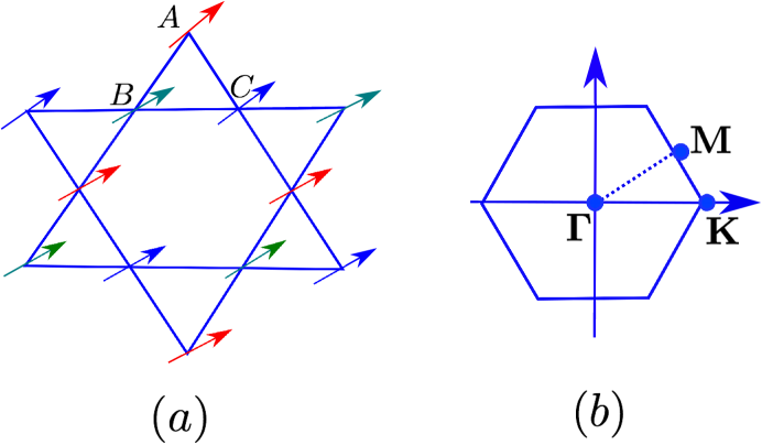
Figure 1: Color online. (a) The three-sublattice ($A,~{}B~{},C$) Kagomé lattice with canted ferromagnet. (b). Brillouin zone of the Kagomé lattice indicating the high symmetry paths ${\bf\Gamma}=(0,0)$; $\mathbb{K}=(2\pi/3,0)$; $\mathbb{M}=(\pi/2,\pi/2\sqrt{3})$.

2 Linear spin wave theory

2.1 Mean-field theory

In the mean-field analysis or large-$S$ limit, the spin operators in Eq. 3 are replaced with classical vectors: $\mathbb{S}_{l}=S\mathbb{n}_{l}$, where $\mathbb{n}_{l}=\left(\sin\theta_{l}\cos\phi_{l},\sin\theta_{l}\sin\phi_{l},\cos\theta_{l}\right)$ is a unit vector. For this model, there is only one possible phase at zero magnetic fields — an easy-axis ferromagnet (FM) resulting from the spontaneously broken $Z_{2}$ symmetry along the $x$-direction. This phase becomes a canted ferromagnet (CFM) for small $H_{z}$. For large $H_{z}$, there is a fully polarized (FP) ferromagnet, with the spins aligned along the $z$-axis. Both ferromagnets are described with $\theta_{l}=\theta$ and $\phi_{l}=0$, hence the classical energy is given by

$$e_{c} =-\zeta\left(1+\Delta\right)\sin^{2}\theta-h_{x}\sin\theta-h_{z}\cos\theta,$$ (4)

where $e_{c}=\mathcal{E}_{c}/\mathcal{N}S^{2}$, $\mathcal{N}$ is the total number of sites, and $\zeta=2,3$ on the Kagomé and the triangular lattices respectively, and $h_{x,z}=H_{x,z}/S$. Minimizing the classical energy with respect to $\theta$ yields

$$h_{x}=\tan\theta_{c}[h_{z}-2\zeta\left(1+\Delta\right)\cos\theta_{c}],$$ (5)

hence

$$e_{c}(\theta_{c}) =\zeta\left(1+\Delta\right)\sin^{2}\theta_{c}-h_{z}\sec\theta_{c},$$ (6)

where $\theta_{c}$ is a function of $h_{x}$. At $h_{x}=0$, we get $h_{z}=h_{F}^{c}\cos\vartheta_{c}$ and the corresponding energy is $e_{c}(\theta_{c}=\vartheta_{c})=-\zeta\left(1+\Delta\right)(1+\cos^{2}\vartheta_{c})$, where $h_{F}^{c}=2\zeta(1+\Delta)$ is the critical field between the CFM and the FP. For $h_{x}\ll 1$, the energy is obtained perturbatively in $h_{x}$:

$$e_{c}=e_{c}(h_{x}=0)+h_{x}\left.\frac{\partial e_{c}(\theta_{c})}{\partial h_{x}}\right|_{h_{x}=0}+\cdots,$$ (7)

where $e_{c}(h_{x}=0)=e_{c}(\theta_{c}=\vartheta_{c})$.

2.2 Holstein-Primakoff transformation

We perform linear spin wave theory (LSWT) by rotating the coordinate about the $y$-axis so that the $z$-axis coincides with the local direction of the classical polarization. The corresponding rotation matrix is

$$\mathcal{R}_{y}(\theta)=\left(\begin{array}[]{ccc}\cos\theta&0&\sin\theta\\ 0&1&0\\ -\sin\theta&0&\cos\theta\\ \end{array}\right).$$ (11)

Next, we employ a three-sublattice Holstein-Primakoff transformation [19] with the bosonic creation and annihilation operators, $a^{\dagger}_{l\alpha}$ and $a_{l\alpha}$ [20] respectively, where $\alpha=A,~{}B,~{}C$ labels the three sublattices on the Kagomé lattice as depicted in Fig. 1(a). After Fourier transform, the linearized momentum space Hamiltonian is given by

$$\mathcal{H}=S\sum_{\mathbb{k},\alpha,\beta}\left(\mathcal{M}_{\alpha\beta}^{0}\delta_{\alpha\beta}+\mathcal{M}_{\alpha\beta}^{-}\right)\left(a_{\mathbb{k}\alpha}^{\dagger}a_{\mathbb{k}\beta}+a_{-\mathbb{k}\alpha}^{\dagger}a_{-\mathbb{k}\beta}\right)$$ (12)

$$+\mathcal{M}_{\alpha\beta}^{+}\left(a_{\mathbb{k}\alpha}^{\dagger}a_{-\mathbb{k}\beta}^{\dagger}+a_{-\mathbb{k}\alpha}a_{\mathbb{k}\beta}\right),$$

where $\alpha,\beta=A,B,C$ and the coefficients are given by $\boldsymbol{\mathcal{M}}^{0}=\xi~{}\rm{diag}\left(1,1,1\right)$, with $\xi=\left(h_{z}\cos\theta+h_{x}\sin\theta\right)/2+\zeta(1+\Delta)\sin^{2}\theta$, and the matrices $\boldsymbol{\mathcal{M}}^{\pm}$ differ only by a pre-factor:

$$\boldsymbol{\mathcal{M}}^{\pm}=-\frac{\chi\pm(1-\Delta)}{2}\boldsymbol{\Omega}$$ (13)

where ${\chi}=(1+\Delta)\cos^{2}\theta$ and $\boldsymbol{\Omega}$ is given by

$$\boldsymbol{\Omega}=\left(\begin{array}[]{ccc}0&\cos k_{1}&\cos k_{2}\\ \cos k_{1}&0&\cos k_{3}\\ \cos k_{2}&\cos k_{3}&0\\ \end{array}\right);$$ (14)

with $k_{j}=\mathbb{k}\cdot\mathbb{\hat{e}}_{j}$; $~{}\mathbb{\hat{e}}_{1}=-\left(1/2,{\sqrt{3}}/2\right);~{}\mathbb{\hat{e}}_{2}=\left(1,0\right);~{}\mathbb{\hat{e}}_{3}=\left(-1/2,{\sqrt{3}}/2\right)$. The eigenvalues of $\boldsymbol{\Omega}$ are given by

$$\omega_{1}=-1;\quad\omega_{2,3}=\frac{1}{2}\left(1\pm\sqrt{1+8g_{\mathbb{k}}}\right);$$ (15)

where $g_{\mathbb{k}}=\cos k_{1}\cos k_{2}\cos k_{3}$. The Hamiltonian 12 is diagonalized in two steps [20]. Firstly, we make a linear transformation

$$a_{\mathbb{k}\alpha}=\sum_{\mu}\mathcal{U}_{\mu\alpha}(\mathbb{k})d_{\mathbb{k}\mu},$$ (16)

where $\mathcal{U}_{\alpha\mu}(\mathbb{k})$ is a unitary matrix constructed from the eigenvectors of $\boldsymbol{\Omega}$ associated with the eigenvalues $\omega_{\alpha}$. Secondly, we apply the Bogoluibov transformation

$$d_{\mathbb{k}\alpha}=u_{\mathbb{k}\alpha}\beta_{\mathbb{k}\alpha}-v_{\mathbb{k}\alpha}\beta_{-\mathbb{k}\alpha}^{\dagger};\quad u_{\mathbb{k}\alpha}^{2}-v_{\mathbb{k}\alpha}^{2}=1.$$ (17)

The resulting Hamiltonian is diagonalized with

$$u_{\mathbb{k}\alpha}^{2}=\frac{1}{2}\left(\frac{A_{\mathbb{k}\alpha}}{{\epsilon}_{\mathbb{k}\alpha}}+1\right);\quad v_{\mathbb{k}\alpha}^{2}=\frac{1}{2}\left(\frac{A_{\mathbb{k}\alpha}}{{\epsilon}_{\mathbb{k}\alpha}}-1\right),$$ (18)

and

$$A_{\mathbb{k}\alpha}=\xi+(1-\Delta)\omega_{\mathbb{k}\alpha}+B_{\mathbb{k}\alpha};~{}B_{\mathbb{k}\alpha}=-\frac{\chi+(1-\Delta)}{2}\omega_{\mathbb{k}\alpha}.$$ (19)

The energy is given by ${\epsilon}_{\mathbb{k}\alpha}=\sqrt{A_{\mathbb{k}\alpha}^{2}-B_{\mathbb{k}\alpha}^{2}}.$ The diagonal Hamiltonian is given by

$$\mathcal{H}=S\sum_{\mathbb{k},\alpha}{\epsilon}_{\mathbb{k}\alpha}\left(\gamma_{\mathbb{k}\alpha}^{\dagger}\gamma_{\mathbb{k}\alpha}+\gamma_{-\mathbb{k}\alpha}^{\dagger}\gamma_{-\mathbb{k}\alpha}\right).$$ (20)

For the triangular lattice, there is only one sublattice. We obtain

$$A_{\mathbb{k}}=\xi+3(1-\Delta)g_{\mathbb{k}}+B_{\mathbb{k}};~{}B_{\mathbb{k}}=-\frac{\chi+3(1-\Delta)}{2}g_{\mathbb{k}},$$ (21)

with $\xi=\left(h_{z}\cos\theta+h_{x}\sin\theta\right)/2+3(1+\Delta)\sin^{2}\theta$, $\chi=3(1+\Delta)\cos^{2}\theta$, and $g_{\mathbb{k}}=(\cos k_{x}+2\cos{k_{x}}/{2}\cos{\sqrt{3}k_{y}}/{2})/3.$ The corresponding Hamiltonian is diagonalized in a similar way, however, without the sublattice indices.

2.3 Excitation spectra

The features of the quantum Kagomé ice hardcore bosons can be understood by analyzing the momentum-dependent eigenfrequencies given by $\varepsilon_{\mathbb{k}\alpha}=2{\epsilon}_{\mathbb{k}\alpha}$. The energy bands for the Kagomé lattice are plotted in Fig. 2 along the Brillouin zone paths in Fig. 1(b) for $\Delta=h_{x,z}=0$ (isotropic limit) and $\Delta=0.25;~{}h_{x}=0;~{}h_{z}=\pm 4.5$. We also show the energy band on the triangular lattice in Fig. 3.

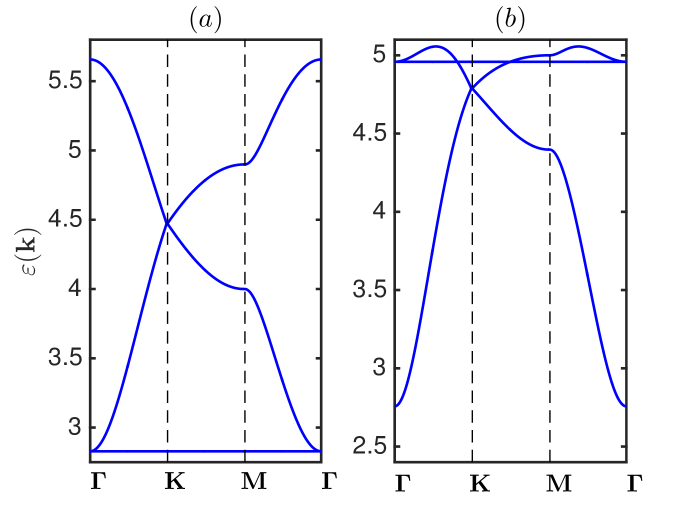
Figure 2: Color online. The plots of the energy bands for the Kagomé lattice at $h_{x}=0$: $\Delta=0=h_{z}$ (a); $\Delta=0.25;~{}h_{z}=\pm 4.5$ (b).

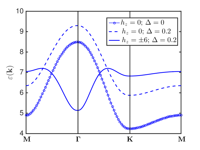
Figure 3: Color online. The plot of the energy band on the triangular lattice at $h_{x}=0$ and several values of $\Delta$ and $h_{z}$. There is only one band for each parameter.

The excitation spectra of Eq. 2 are fully gapped on both lattices for all $\Delta$ between $0$ and $1$ for $h_{x,z}=0$. The gap persists at all values of the magnetic field $h_{z}\leq h_{F}^{c}$ and $h_{x}=0$. The absence of a zero (soft) mode in the quantum Kagomé ice hardcore bosons is a direct consequence of the discrete $Z_{2}$ symmetry of Eq. 2. For the triangular lattice, a roton minimum occurs at the corners of the Brillouin zone for $\Delta=h_{x,z}=0$, i.e., at $\mathbb{Q}_{\bf K}=(\pm 4\pi/3,0)$ and the symmetry related points, whereas the dispersion has a maximum peak at $\mathbb{Q}_{\bf\Gamma}=(0,0)$. This is in stark contrast to pure U(1)-invariant XY model.

2.4 Ground state energy

The spin wave correction to the mean field energy is given by

$$\Delta\mathcal{E}=\mathcal{E}_{g}-\mathcal{E}_{c}=S\sum_{\mathbb{k},\alpha}[{\epsilon}_{\mathbb{k}\alpha}-\xi].$$ (22)

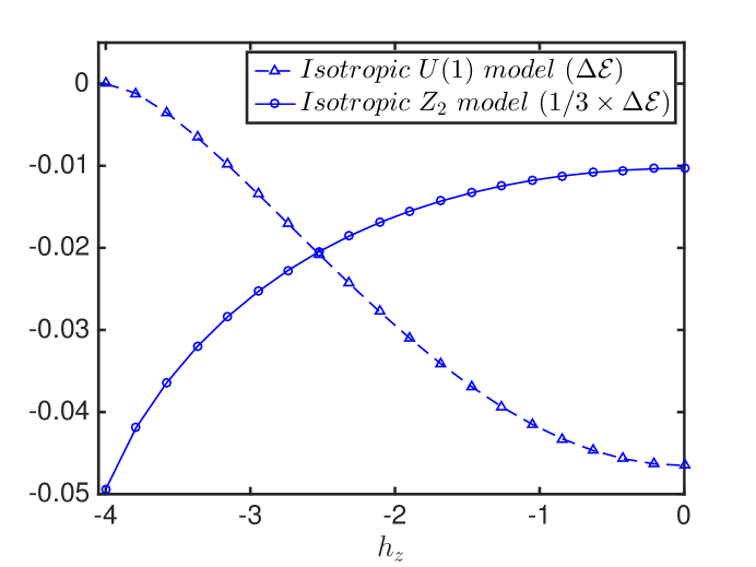
Figure 4: Color online. The spin wave zero point quantum correction as a function of $h_{z}$ on the Kagomé lattice at the isotropic $Z_{2}$-invariant limit $\Delta=h_{x}=0$; $S=1/2$. The U(1)-invariant model is plotted at the corresponding isotropic limit.

The correction to the ground state energy as a function of $h_{z}$ is plotted in Fig. 4 for the Kagomé lattice. The triangular lattice has a similar trend. We see that the trend of the quantum Kagomé ice hardcore bosons is different from that of the U(1)-invariant XY model. In particular, the energy of the isotropic $Z_{2}$-invariant model at $\Delta=h_{x}=0$ does not vanish at the saturated point $h_{z}=h_{F}^{c}$. The estimated ground state energy on the Kagomé lattice at the isotropic point $\Delta=h_{z,x}=0$ is $\mathcal{E}_{g}=-0.5309$. Finite temperature QMC simulation 1 for a relatively large cluster $V=24\times 24\times 3$ spins at inverse-temperature $\beta=100$ gives $\mathcal{E}_{g}=-0.5359(2)$, in good agreement with linear spin wave theory. For the triangular lattice, linear spin wave theory gives $\mathcal{E}_{g}=-0.7791$ [21]; there is no QMC result in this case.

2.5 Particle and condensate densities

We now study the ground state properties of Eq. 3 by probing the sublattice magnetizations, which will quantify the strengths of quantum fluctuations in this model. We first analyze the Kagomé lattice, the triangular lattice follows a similar pattern. For the Kagomé lattice, the sublattice magnetizations are equivalent, the total magnetizations per site are given by

$$\langle S_{z}\rangle=-\frac{1}{S\mathcal{N}}\frac{\partial\mathcal{E}_{SW}(h_{z},h_{x}=0)}{\partial h_{z}},$$ (23)

$$\langle S_{x}\rangle=-\frac{1}{S\mathcal{N}}\left.\frac{\partial\mathcal{E}_{SW}(h_{z},h_{x})}{\partial h_{x}}\right|_{h_{x}=0}.$$ (24)

Using Eq. 22 we obtain

$$\langle S_{z}\rangle=S\cos\vartheta_{c}+\frac{\cos\vartheta_{c}}{2\zeta}\frac{1}{\mathcal{N}}\sum_{\mathbb{k}\alpha}(\tilde{A}_{\mathbb{k}\alpha}-\tilde{B}_{\mathbb{k}\alpha})\frac{\omega_{\mathbb{k}\alpha}}{\tilde{\epsilon}_{\mathbb{k}\alpha}}.$$ (25)

To linear order in $h_{x}$ we find

$$\langle S_{x}\rangle=S\sin\vartheta_{c}-\frac{\cos^{2}\vartheta_{c}}{2\zeta\sin\vartheta_{c}}\frac{1}{\mathcal{N}}\sum_{\mathbb{k}\alpha}(\tilde{A}_{\mathbb{k}\alpha}-\tilde{B}_{\mathbb{k}\alpha})\frac{\omega_{\mathbb{k}\alpha}}{\tilde{\epsilon}_{\mathbb{k}\alpha}}$$ (26)

$$-\frac{1}{2\sin\vartheta_{c}}\frac{1}{\mathcal{N}}\sum_{\mathbb{k}\alpha}\bigg{[}\frac{\tilde{A}_{\mathbb{k}\alpha}}{\tilde{\epsilon}_{\mathbb{k}\alpha}}-1\bigg{]}.$$

where $\tilde{A}_{\mathbb{k}\alpha}=A_{\mathbb{k}\alpha}(h_{x}=0)$, etc. As seen in Eqs. 25 and 26, the denominator in these expressions correspond to the gapped energy spectrum. We define the particle density $\rho$ and the “condensate density” at $\mathbb{k}_{\Gamma}=0$ as $\rho=S+\langle S_{z}\rangle$ and $\rho_{0}=\langle S_{x}\rangle^{2}$ respectively. In LSWT we find

$$\rho_{0}=(S\sin\vartheta_{c})^{2}-S\frac{\cos^{2}\vartheta_{c}}{\zeta}\frac{1}{\mathcal{N}}\sum_{\mathbb{k}\alpha}(\tilde{A}_{\mathbb{k}\alpha}-\tilde{B}_{\mathbb{k}\alpha})\frac{\omega_{\mathbb{k}\alpha}}{\tilde{\epsilon}_{\mathbb{k}\alpha}}$$ (27)

$$-S\frac{1}{\mathcal{N}}\sum_{\mathbb{k}\alpha}\bigg{[}\frac{\tilde{A}_{\mathbb{k}\alpha}}{\tilde{\epsilon}_{\mathbb{k}\alpha}}-1\bigg{]}.$$

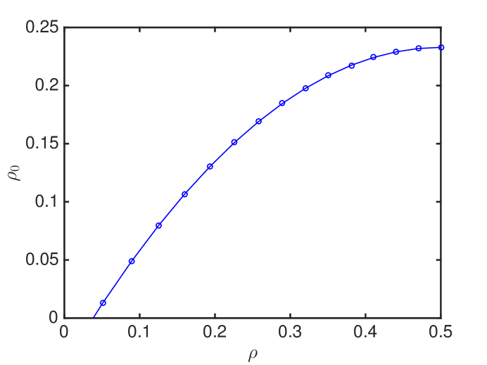
Figure 5: Color online. The spin wave condensate density $\rho_{0}$ against the particle density $\rho$ on the Kagomé lattice at $h_{x}=\Delta=0$ and $S=1/2$.

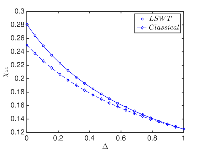
Figure 6: Color online. The plot of the classical and the spin wave quantum susceptibilities as a function of $\Delta$ for the Kagomé lattice at $S=1/2$.

The corresponding expressions for the triangular lattice are similar to the Kagomé lattice without the sublattice summation. Figure 5 shows the plot of the condensate against the particle density at $\Delta=0$ (isotropic $Z_{2}$-invariant XY model) for on the Kagomé lattice. At half filling ($\rho=0.5$ or $h_{x,z}=\Delta=0$), the estimated values of the order parameter for the Kagomé lattice is $\langle S_{x}\rangle=0.4829$ and $\rho_{0}=\langle S_{x}\rangle^{2}$. Finite temperature QMC simulation 1 for a relatively large cluster $V=24\times 24\times 3$ spins at inverse-temperature $\beta=24$ gives $\langle S_{x}\rangle=0.4785(2)$. For the triangular lattice, linear spin wave theory gives $\langle S_{x}\rangle=0.4902$, which is closer to the mean-field value $\langle S_{x}\rangle=0.5000$, there is no QMC result in this case. Clearly, the gapped energy spectrum of Eq. 26 enhances the thermodynamic quantities.

The out-of-plane magnetic susceptibility, $\chi_{zz}$, is another important measurable quantity as it relates to the compressibility of bosons. It is given by

$$\chi_{zz}=\frac{1}{S}\left.\frac{\partial\langle S_{z}\rangle}{\partial h_{z}}\right|_{h_{z}=0}.$$ (28)

We find

$$\chi_{zz}=\chi_{zz}^{c}+\frac{1}{4\zeta^{2}(1+\Delta)S}\frac{1}{\mathcal{N}}\sum_{\mathbb{k}\alpha}(\bar{A}_{\mathbb{k}\alpha}-\bar{B}_{\mathbb{k}\alpha})\frac{\omega_{\mathbb{k}\alpha}}{\bar{\epsilon}_{\mathbb{k}\alpha}},$$ (29)

where $\chi_{zz}^{c}=[2\zeta(1+\Delta)]^{-1}$ is the classical susceptibility and $\bar{A}_{\mathbb{k}\alpha}=A_{\mathbb{k}\alpha}(h_{x,z}=0)$, etc. The plot of $\chi_{zz}^{c}$ and $\chi_{zz}$ as a function of $\Delta$ are shown in Fig. 6 for the Kagomé lattice. The triangular lattice has a similar trend. The classical and the quantum susceptibilities coincide as $\Delta\to 1$, corresponding to the fully polarized $S_{x}$-ferromagnet. The estimated values of $\chi_{zz}$ at the isotropic $Z_{2}$-invariant limit, $\Delta=0$ for the Kagomé is $\chi_{zz}=0.2807$. Finite temperature QMC simulation 1 for a large cluster $V=24\times 24\times 3$ spins at inverse-temperature $\beta=24$ gives $\chi_{zz}=0.2785(2)$. For the triangular lattice, linear spin wave theory gives $\chi_{zz}=0.1799$, and the mean-field value $\chi_{zz}=1/6$; again there is no QMC result in this case. In contrast to the U(1)-invariant model [10, 12, 14, 11, 15, 16, 13, 17, 18], we see that quantum fluctuation increases the classical susceptibility away from $\Delta=1$.

2.6 Dynamical structure factors

Furthermore, we explore the nature of the quantum Kagomé ice hardcore bosons by studying the dynamical structure factor, which is an important quantity in experiments for characterizing the ground state properties of a quantum system. The spin structure factor is given by the Fourier transform of the equal-time spin-spin correlation function

$$\mathcal{S}^{\mu\nu}(\mathbb{k})=\frac{1}{\mathcal{N}}\sum_{l,m}e^{i\mathbb{k}\cdot(\mathbb{r}_{l}-\mathbb{r}_{m})}\langle S_{l}^{\mu}S_{m}^{\nu}\rangle,$$ (30)

where $\mu,\nu=(x,y,z)$ label the components of the spins and $S_{l}^{\mu}=\sum_{\alpha}S_{l\alpha}^{\mu}$ on the Kagomé lattice, $\alpha$ labels the sublattices. We restrict the calculation of the structure factors to the case of half-filling ($\rho=0.5$) or zero magnetic fields ( $h_{x,z}=0$).

The momentum distribution is related to the off-diagonal static structure factor $\mathcal{S}^{\pm}(\mathbb{k})$. We have $\langle S_{l}^{+}S_{m}^{-}\rangle=\langle S_{l}^{x}S_{m}^{x}\rangle+\langle S_{l}^{y}S_{m}^{y}\rangle+\langle S_{l}^{z}\rangle\delta_{lm}$. At $h_{x,z}=0$, $\theta=\pi/2$, hence rotation about the $y$-axis gives $S_{l}^{x}\to S_{l}^{\prime z},~{}S_{l}^{z}\to-S_{l}^{\prime x},$ and $S_{l}^{y}\to S_{l}^{\prime y}$. The off-diagonal structure factor in the rotated coordinate up to order $S$ is given by $\mathcal{S}^{\pm}(\mathbb{k})=\langle S_{\mathbb{k}}^{\prime z}S_{-\mathbb{k}}^{\prime z}\rangle+\langle S_{\mathbb{k}}^{\prime y}S_{-\mathbb{k}}^{\prime y}\rangle.$ At $\mathbb{k}_{\bf\Gamma}=0$, $\mathcal{S}^{\pm}(\mathbb{k})$ is related to the order parameter by $\rho_{0}=\mathcal{S}^{\pm}(\mathbb{k}_{\Gamma})/\mathcal{N}$ as $\mathcal{N}\to\infty$.

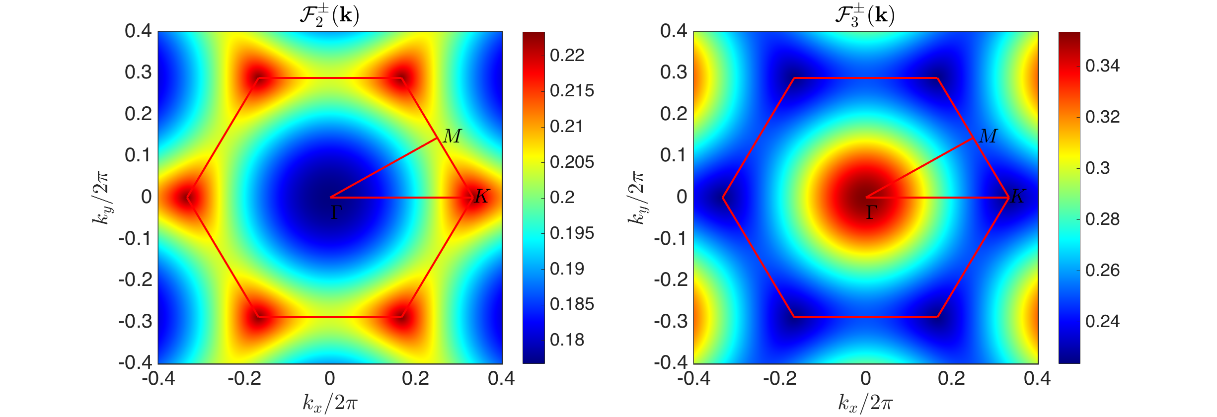
Figure 7: Color online. The plot of the off-diagonal form factor $\mathcal{F}^{\pm}(\mathbb{k})$ for the two dispersive bands on the Kagomé lattice at $S=1/2$; $\Delta=h_{x,z}=0$.

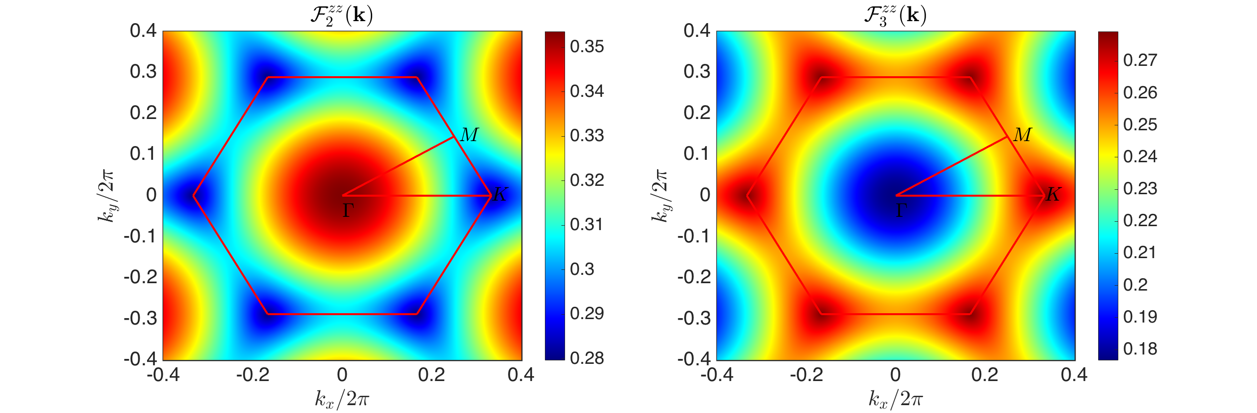
Figure 8: Color online. The plot of the out-of-plane form factor $\mathcal{F}^{zz}(\mathbb{k})$ for the two dispersive bands on the Kagomé lattice at $S=1/2$; $\Delta=h_{x,z}=0$.

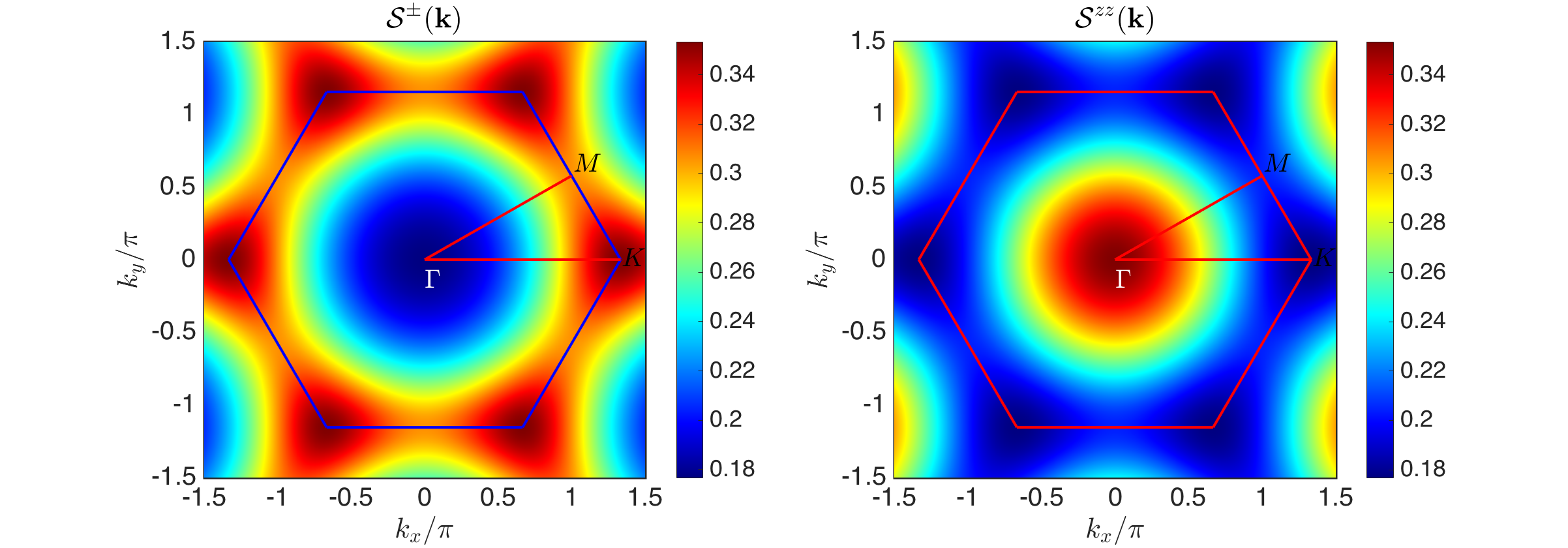
Figure 9: Color online. The plot of the off-diagonal structure factor $\mathcal{S}^{\pm}(\mathbb{k})$ and out-of-plane structure factor $\mathcal{S}^{zz}(\mathbb{k})$ for the triangular lattice at $S=1/2$; $\Delta=h_{x,z}=0$.

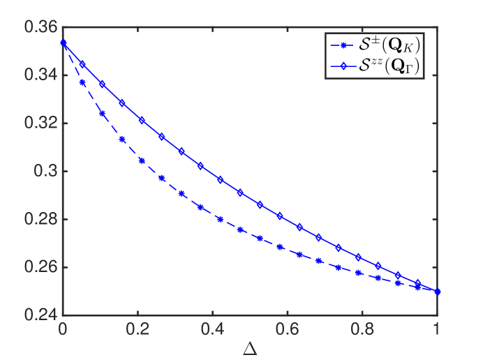
Figure 10: Color online. The plot of the structure factors in Eqs. 34 and 35 as a function of $\Delta$ at $h_{x,z}=0$, $S=1/2$.

For the Kagomé lattice we find that the off-diagonal structure factor for $\mathbb{k}\neq\mathbb{k}_{\Gamma}$ and the out-of-plane structure factor are given by

$$\mathcal{S}^{\pm}(\mathbb{k})=\sum_{\mu}\mathcal{F}_{\mu}^{\pm}(\mathbb{k}),~{}~{}\mathcal{S}^{zz}(\mathbb{k})=\sum_{\mu}\mathcal{F}_{\mu}^{zz}(\mathbb{k}),$$ (31)

where $\mathcal{F}_{\mu}^{\pm}(\mathbb{k})=S(u_{\mu\mathbb{k}}+v_{\mu\mathbb{k}})^{2}/{2}\sum_{\alpha\alpha^{\prime}}\mathcal{U}_{\mu\alpha}(\mathbb{k})\mathcal{U}_{\mu\alpha^{\prime}}(\mathbb{k})$ and $\mathcal{F}_{\mu}^{zz}(\mathbb{k})=S(u_{\mu\mathbb{k}}-v_{\mu\mathbb{k}})^{2}/{2}\sum_{\alpha\alpha^{\prime}}\mathcal{U}_{\mu\alpha}(\mathbb{k})\mathcal{U}_{\mu\alpha^{\prime}}(\mathbb{k})$. For the triangular lattice, the explicit expressions are

$$\mathcal{S}^{\pm}(\mathbb{k})=\frac{S}{2}(u_{\mathbb{k}}+v_{\mathbb{k}})^{2}=\frac{S}{2}\left(\frac{A_{\mathbb{k}}+B_{\mathbb{k}}}{\sqrt{A_{\mathbb{k}}^{2}-B_{\mathbb{k}}^{2}}}\right),$$ (32)

$$\mathcal{S}^{zz}(\mathbb{k})=\frac{S}{2}(u_{\mathbb{k}}-v_{\mathbb{k}})^{2}=\frac{S}{2}\left(\frac{A_{\mathbb{k}}-B_{\mathbb{k}}}{\sqrt{A_{\mathbb{k}}^{2}-B_{\mathbb{k}}^{2}}}\right).$$ (33)

The denominator of Eqs. 32 and 33 correspond to the energy spectrum, which is gapped in the entire Brillouin zone. In Figs. 7 and 8 we have shown the off-diagonal form factor $\mathcal{F}^{\pm}(\mathbb{k})$ and the out-of-plane form factor $\mathcal{F}^{zz}(\mathbb{k})$ for the two dispersive bands on the Kagomé lattice. Figure 9 shows the off-diagonal and the out-of-plane structure factors on the triangular lattice. The solid hexagons denote the respective Brillouin zones for the two lattices. For the Kagomé lattice, the momentum distribution shows noticeable non-divergent sharp peaks at the center and corners of the Brillouin zones, whereas for the triangular lattice we observe non-divergent peaks at $\mathbb{Q}_{\bf K}=(\pm 4\pi/3,0)$ and symmetry related points. This is due to the roton minima of the excitation spectrum in at $\mathbb{Q}_{\bf K}=(\pm 4\pi/3,0)$ as opposed to a divergent peak at $\mathbb{k}_{\bf\Gamma}=0$ in the U(1)-invariant model [10, 11, 12, 13]. On the other hand, the out-of-plane structure factor, $\mathcal{S}^{zz}(\mathbb{k})$, shows a non-divergent sharp peak at $\mathbb{k}_{\bf\Gamma}=0$. At $\mathbb{Q}_{\bf K}=(\pm 4\pi/3,0)$ and $\mathbb{Q}_{\bf\Gamma}=(0,0)$ we have

$$\mathcal{S}^{\pm}(\mathbb{Q}_{\bf K})=S\sqrt{\frac{1+\Delta}{2(1+3\Delta)}},$$ (34)

$$\mathcal{S}^{zz}(\mathbb{Q}_{\bf\Gamma})=\frac{S}{\sqrt{2(1+\Delta)}}.$$ (35)

Figure 10 shows the trend of $\mathcal{S}^{\pm}(\mathbb{Q}_{\bf K})$ and $\mathcal{S}^{zz}(\mathbb{Q}_{\bf\Gamma})$ as a function of $\Delta$.

3 Conclusion

We have shown that linear spin wave theory works remarkably well in the description of the quantum Kagomé ice hardcore bosons. Due to the $Z_{2}$-invariance of the quantum Kagomé ice hardcore boson model, the excitation spectra is fully gapped at all momenta and the resulting occupation number is very small. The gapped nature of the excitation spectrum enhances the estimated values of the thermodynamic quantities. We showed that these values are in very good agreement with finite temperature quantum Monte Carlo (QMC) simulations. We observed Bragg peaks in the structure factors at the center and corners of the Brillouin zone for the Kagomé lattice. This is a special feature of the $Z_{2}$-invariance of the Hamiltonian. For the triangular lattice, we also observed Bragg peaks in the structure factors at the corners of the Brillouin zone. These are consequences of the roton minimum in the energy spectrum. Although we have partially studied this model numerically, the results presented in this paper are sufficient to understand the nature of the quantum Kagomé ice hardcore bosons. However, it would be interesting to explore other properties of this model by an explicit zero temperature QMC analysis.

References

References

• [1] Y.-P. Huang, G. Chen, and M. Hermele, Phys. Rev. Lett. 112, 167203 (2014).
• [2] M. J. P. Gingras and P. A. McClarty, Reports on Progress in Physics 77, 056501 (2014).
• [3] J. Carrasquilla, Z. Hao, and R. G. Melko, Nature Communications 6, 7421 (2015).
• [4] S. A. Owerre, A. A. Burkov, and R. G. Melko, Phys. Rev. B 93, 144402 (2016).
• [5] M. Greiner, et al., Nature 415, 39 (2002).
• [6] L.-M. Duan, E. Demler, and M. D. Lukin, Phys. Rev. Lett. 91, 090402 (2003).
• [7] J. Struck et al., Nature Physics 9, 738 (2013).
• [8] O. Kyriienko, et al., EPL 109, 57003 (2015), J. P. Eisenstein and A. H. MacDonald, Nature 432, 691 (2004), A. A. Burkov and A. H. MacDonald, Phys. Rev. B 66, 115320 (2002).
• [9] T. Matsubara and H. Matsuda, Prog. Theor. Phys. 16, 569 (1956).
• [10] K. Bernardet, et al., Phys. Rev. B 65, 104519 (2002).
• [11] A. W. Sandvik and C. J. Hamer, Phys. Rev. B 60, 6588 (1999); I. Hen and M. Rigol, Phys. Rev. B 80, 134508 (2009).
• [12] T. Coletta, N. Laflorencie, and F. Mila, Phys. Rev. B 85, 104421 (2012).
• [13] G. Gomez and J. D. Joannopolos, Phys. Rev. B 36, 8707 (1987).
• [14] A. W. Sandvik and R. G. Melko, Ann. Phys. 321, 1651 (2006).
• [15] S. Fujiki, D. D. Betts, Can. J. Phys. 64, 876 (1986).
• [16] H. Nishimori, and H. Nakanishi, J. Phys. Soc. Jpn. 57, 626 (1988).
• [17] Z. Weihong, J. Oitmaa, and C. J. Hamer, Phys. Rev. B 44, 11869 (1991); J. Oitmaa, C. J. Hamer, and Z. Weihong, Phys. Rev. B 45, 9834 (1992).
• [18] C. J. Hamer, J. Oitmaa, and Z. Weihong, Phys. Rev. B 43, 10789 (1991).
• [19] T. Holstein and H. Primakoff, Phys. Rev. 58, 1098 (1940).
• [20] A. B. Harris, C. Kallin, and A. J. Berlinsky, Phys. Rev. B 45, 2899 (1992).
• [21] S. A. Owerre, Phys. Rev. B 93, 094436 (2016).