Grid Based Nonlinear Filtering Revisited:
Recursive Estimation & Asymptotic Optimality

Abstract

We revisit the development of grid based recursive approximate filtering of general Markov processes in discrete time, partially observed in conditionally Gaussian noise. The grid based filters considered rely on two types of state quantization: The Markovian type and the marginal type. We propose a set of novel, relaxed sufficient conditions, ensuring strong and fully characterized pathwise convergence of these filters to the respective MMSE state estimator. In particular, for marginal state quantizations, we introduce the notion of conditional regularity of stochastic kernels, which, to the best of our knowledge, constitutes the most relaxed condition proposed, under which asymptotic optimality of the respective grid based filters is guaranteed. Further, we extend our convergence results, including filtering of bounded and continuous functionals of the state, as well as recursive approximate state prediction. For both Markovian and marginal quantizations, the whole development of the respective grid based filters relies more on linear-algebraic techniques and less on measure theoretic arguments, making the presentation considerably shorter and technically simpler.

   Keywords. Nonlinear Filtering, Grid Based Filtering, Approximate Filtering, Markov Chains, Markov Processes, Sequential Estimation, Change of Probability Measures.

1 Introduction

It is well known that except for a few special cases [1, 2, 3, 4, 5], general nonlinear filters of partially observable Markov processes (or Hidden Markov Models (HMMs)) do not admit finite dimensional (recursive) representations [6, 7]. Nonlinear filtering problems, though, arise naturally in a wide variety of important applications, including target tracking [8, 9], localization and robotics [10, 11], mathematical finance [12] and channel prediction in wireless sensor networks [13], just to name a few. Adopting the Minimum Mean Square Error (MMSE) as the standard optimality criterion, in most cases, the nonlinear filtering problem results in a dynamical system in the infinite dimensional space of measures, making the need for robust approximate solutions imperative.

Approximate nonlinear filtering methods can be primarily categorized into two major groups [14]: local and global. Local methods include the celebrated extended Kalman filter [15], the unscented Kalman filter [16], Gaussian approximations [17], cubature Kalman filters [18] and quadrature Kalman filters [19]. These methods are mainly based on the local “assumed form of the conditional density” approach, which dates back to the 1960’s [20]. Local methods are characterized by relatively small computational complexity, making them applicable in relatively higher dimensional systems. However, they are strictly suboptimal and, thus, they at most constitute efficient heuristics, but without explicit theoretical guarantees. On the other hand, global methods, which include grid based approaches (relying on proper quantizations of the state space of the state process [21, 22, 23]) and Monte Carlo approaches (particle filters and related methods [24]), provide approximations to the whole posterior measure of the state. Global methods possess very powerful asymptotic optimality properties, providing explicit theoretical guarantees and predictable performance. For that reason, they are very important both in theory and practice, either as solutions, or as benchmarks for the evaluation of suboptimal techniques. The main common disadvantage of global methods is their high computational complexity as the dimensionality of the underlying model increases. This is true both for grid based and particle filtering techniques [25, 26, 27, 28, 29].

In this paper, we focus on grid based approximate filtering of Markov processes observed in conditionally Gaussian noise, constructed by exploiting uniform quantizations of the state. Two types of state quantizations are considered: the Markovian and the marginal ones (see [21] and/or Section 3). Based on existing results [7, 14, 21], one can derive grid based, recursive nonlinear filtering schemes, exploitting the properties of the aforementioned types of state approximations. The novelty of our work lies in the development of an original convergence analysis of those schemes, under generic assumptions on the expansiveness of the observations (see Section 2). Our contributions can be summarized as follows:

1) For marginal state quantizations, we propose the notion of conditional regularity of Markov kernels (Definition 2), which is an easily verifiable condition for guaranteeing strong asymptotic consistency of the resulting grid based filter. Conditional regularity is a simple and relaxed condition, in contrast to more complicated and potentially stronger conditions found in the literature, such as the Lipschitz assumption imposed on the stochastic kernel(s) of the underlying process in [21].

2) Under certain conditions, we show that all grid based filters considered here converge to the true optimal nonlinear filter in a strong and controllable sense (Theorems 3 and 4). In particular, the convergence is compact in time and uniform in a measurable set occurring with probability almost $1$; this event is completely characterized in terms of the filtering horizon and the dimensionality of the observations.

3) We show that all our results can be easily extended in order to support filters of functionals of the state and recursive, grid based approximate prediction (Theorem 5). More specifically, we show that grid based filters are asymptotically optimal as long as the state functional is bounded and continuous; this is a typical assumption (see also [7, 23, 30]). Of course, this latter assumption is in addition to and independent from any other condition (e.g., conditional regularity) imposed on the structure of the partially observable system under consideration. In a companion paper [13], this simple property has been proven particularly useful, in the context of channel estimation in wireless sensor networks. The assumption of a bounded and continuous state functional is more relaxed as compared to the respective bounded and Lipschitz assumption found in [21].

Another novel aspect of our contribution is that our original theoretical development is based more on linear-algebraic arguments and less on measure theoretic ones, making the presentation shorter, clearer and easy to follow.

Relation to the Literature

In this paper, conditional regularity is presented as a relaxed sufficient condition for asymptotic consistency of discrete time grid based filters, employing marginal state quantizations. Another set of conditions ensuring asymptotic convergence of state approximations to optimal nonlinear filters are the Kushner’s local consistency conditions (see, example, [23, 22]). These refer to Markov chain approximations for continuous time Gaussian diffusion processes and the related standard nonlinear filtering problem.

It is important to stress that, as it can be verified in Section IV, the constraints which conditional regularity imposes on the stochastic kernel of the hidden Markov process under consideration are general and do not require the assumption of any specific class of hidden models. In this sense, conditional regularity is a nonparametric condition for ensuring convergence to the optimal nonlinear filter. For example, hidden Markov processes driven by strictly non-Gaussian noise are equally supported as their Gaussian counterparts, provided the same conditions are satisfied, as suggested by conditional regularity (see Section IV). Consequently, it is clear that conditional regularity advocated in this paper is different in nature than Kushner’s local consistency conditions [23, 22]. In fact, putting the differences between continuous and discrete time aside, conditional regularity is more general as well.

Convergence of discrete time approximate nonlinear filters (not necessarily recursive) is studied in [31]. No special properties of the state are assumed, such as the Markov property; it is only assumed that the state is almost surely compactly supported. In this work, the results of [31] provide the tools for showing asymptotic optimality of grid base, recursive approximate estimators. Further, our results have been leveraged in [13, 32], showing asymptotic consistency of sequential spatiotemporal estimators/predictors of the magnitude of the wireless channel over a geographical region, as well as its variance. The estimation is based on limited channel observations, obtained by a small number of sensors.

The paper is organized as follows. In Section II, we define the system model under consideration and formulate the respective filtering approximation problem. In Section III, we present useful results on the asymptotic characterization of the Markovian and marginal quantizations of the state (Lemmata 2 and 4). Exploiting these results, Section IV is devoted to: (a) Showing convergence of the respective (not necessarily finite dimensional) grid based filters (Theorem 2). (b) Derivation of the respective recursive, asymptotically optimal filtering schemes, based on the Markov property and any other conditions imposed on the state (Theorem 3 and Lemmata 5 and 6, leading to Theorem 4). Extensions to the main results are also presented (Theorem 5), and recursive filter performance evaluation is also discussed (Theorem 6). Some analytical examples supporting our investigation are discussed in Section V, along with some numerical simulations. Finally, Section VI concludes the paper.

Notation: In the following, the state vector will be represented as $X_{t}$, its innovative part as $W_{t}$ (if exists), its approximations as $X_{t}^{L_{S}}$, and all other matrices and vectors, either random or not, will be denoted by boldface letters (to be clear by the context). Real valued random variables will be denoted by uppercase letters. Calligraphic letters and formal script letters will denote sets and $\sigma$-algebras, respectively. For any random variable (same for vector) $Y$, $\sigma\left\{Y\right\}$ will denote the $\sigma$-algebra generated by $Y$. The essential supremum (with respect to some measure - to be clear by the context) of a function $f\left(\cdot\right)$ over a set ${\cal A}$ will be denoted by $\mathrm{ess}\hskip 1.99997pt\mathrm{sup}_{x\in{\cal A}}f\left(x\right)$. The operators $\left(\cdot\right)^{\boldsymbol{T}}$, $\lambda_{min}\left(\cdot\right)$ and $\lambda_{max}\left(\cdot\right)$ will denote transposition, minimum and maximum eigenvalue, respectively. The $\ell_{p}$-norm of a vector $\boldsymbol{x}\in\mathbb{R}^{n}$ is $\left\|\boldsymbol{x}\right\|_{p}\triangleq\left(\sum_{i=1}^{n}\left|x\left(i\right)\right|^{p}\right)^{1/p}$, for all naturals $p\geq 1$. For any Euclidean space $\mathbb{R}^{N}$, ${\bf I}_{N}$ will denote the respective identity operator. For collections of sets $\left\{{\cal A},{\cal B}\right\}$ and $\left\{{\cal C},{\cal D}\right\}$, the usual Cartesian product is overloaded by defining $\left\{{\cal A},{\cal B}\right\}\times\left\{{\cal C},{\cal D}\right\}\triangleq\left\{{\cal A}\times{\cal C},{\cal A}\times{\cal D},{\cal B}\times{\cal C},{\cal B}\times{\cal D}\right\}$. Additionally, we employ the identifications $\mathbb{R}_{+}\equiv\left[0,\infty\right)$, $\mathbb{R}_{++}\equiv\left(0,\infty\right)$, $\mathbb{N}^{+}\equiv\left\{1,2,\ldots\right\}$, $\mathbb{N}_{n}^{+}\equiv\left\{1,2,\ldots,n\right\}$ and $\mathbb{N}_{n}\equiv\left\{0\right\}\cup\mathbb{N}_{n}^{+}$, for any positive natural $n$.

2 System Model & Problem Formulation

2.1 System Model & Technical Assumptions

All stochastic processes defined below are defined on a common complete probability space (the base space), defined by a triplet $\left(\Omega,\mathscr{F},{\cal P}\right)$. Also, for a set ${\cal A}$, $\mathscr{B}\left({\cal A}\right)$ denotes the respective Borel $\sigma$-algebra.

Let $X_{t}\in\mathbb{R}^{M\times 1}$ be Markov with known dynamics (stochastic kernel)

$${\cal K}_{t}:\mathscr{B}\left(\mathbb{R}^{M\times 1}\right)\times\mathbb{R}^{M\times 1}\mapsto\left[0,1\right],\quad t\in\mathbb{N},$$ (1)

which, together with an initial probability measure ${\cal P}_{X_{-1}}$ on $\left(\mathbb{R}^{M\times 1},\mathscr{B}\left(\mathbb{R}^{M\times 1}\right)\right)$, completely describe its stochastic behavior. Generically, the state is assumed to be compactly supported in $\mathbb{R}^{M\times 1}$, that is, for all $t\in\left\{-1\right\}\cup\mathbb{N},X_{t}\in{\cal Z}\subset\mathbb{R}^{M\times 1}$, ${\cal P}-a.s.$. We may also alternatively assume the existence of an explicit state transition model describing the temporal evolution of the state, as

$$X_{t}\triangleq f_{t}\left(X_{t-1},W_{t}\right)\in{\cal Z},\quad\forall t\in\mathbb{N},$$ (2)

where, for each $t$, $f_{t}:{\cal Z}\times{\cal W}\overset{a.s.}{\mapsto}{\cal Z}$ constitutes a measurable nonlinear state transition mapping with somewhat “favorable” analytical behavior (see below) and $W_{t}\equiv W_{t}\left(\omega\right)\in{\cal W}\subseteq\mathbb{R}^{M_{W}\times 1}$, for $t\in\mathbb{N}$, $\omega\in\Omega$, denotes a white noise process with state space ${\cal W}$. The recursion defined in (2) is initiated by choosing $X_{-1}\sim{\cal P}_{X_{-1}}$, independently of $W_{t}$.

The state $X_{t}$ is partially observed through the conditionally Gaussian process

$$\mathbb{R}^{N\times 1}\ni\left.{\bf y}_{t}\right|X_{t}\overset{i.i.d.}{\sim}{\cal N}\left(\boldsymbol{\mu}_{t}\left(X_{t}\right),\boldsymbol{\Sigma}_{t}\left(X_{t}\right)+\sigma_{\boldsymbol{\Sigma}}^{2}{\bf I}_{N}\right),$$ (3)

$\sigma_{\boldsymbol{\Sigma}}\geq 0$, with conditional means and variances known apriori, for all $t\in\mathbb{N}$. Additionally, we assume that $\boldsymbol{\Sigma}_{t}\left(X_{t}\right)\succ{\bf 0}$, with $\boldsymbol{\Sigma}_{t}:{\cal Z}\mapsto{\cal D}_{\boldsymbol{\Sigma}}$, for all $t\in\mathbb{N}$, where ${\cal D}_{\boldsymbol{\Sigma}}\subset\mathbb{R}^{N\times N}$ is bounded. The observations (3) can also be rewritten in the canonical form ${\bf y}_{t}\equiv\boldsymbol{\mu}_{t}\left(X_{t}\right)+\sqrt{{\bf C}_{t}\left(X_{t}\right)}\boldsymbol{u}_{t}$, for all $t\in\mathbb{N}$, where $\boldsymbol{u}_{t}\equiv\boldsymbol{u}_{t}\left(\omega\right)$ constitutes a standard Gaussian white noise process and, for all $\boldsymbol{x}\in{\cal Z}$, ${\bf C}_{t}\left(\boldsymbol{x}\right)\triangleq\boldsymbol{\Sigma}_{t}\left(\boldsymbol{x}\right)+\sigma_{\boldsymbol{\Sigma}}^{2}{\bf I}_{N}$. The process $\boldsymbol{u}_{t}$ is assumed to be mutually independent of $X_{-1}$, and of the innovations $W_{t}$, in case $X_{t}\equiv f_{t}\left(X_{t-1},W_{t}\right)$.

The class of partially observable systems described above is very wide, containing all (first order) Hidden Markov Models (HMMs) with compactly supported state processes and conditionally Gaussian measurements. Hereafter, without loss of generality and in order to facilitate the presentation, we will assume stationarity of state transitions, dropping the subscript “$t$” in the respective stochastic kernels and/or transition mappings. However, we should mention that all subsequent results hold true also for the nonstationary case, if one assumes that any condition hereafter imposed on the mechanism generating $X_{t}$ holds for all $t\in\mathbb{N}$, that is, for all different “modes” of the state process. As in [31], the following additional technical assumptions are made.

Assumption 1: (Boundedness) The quantities $\lambda_{max}\left({\bf C}_{t}\left(\boldsymbol{x}\right)\right)$, $\left\|\boldsymbol{\mu}_{t}\left(\boldsymbol{x}\right)\right\|_{2}$ are each uniformly upper bounded both with respect to $t\in\mathbb{N}$ and $\boldsymbol{x}\in{\cal X}$, with finite bounds $\lambda_{sup}$ and $\mu_{sup}$, respectively. For technical reasons, it is also true that $\lambda_{inf}\triangleq\inf_{t\in\mathbb{N}}\inf_{\boldsymbol{x}\in{\cal X}}\lambda_{min}\left({\bf C}_{t}\left(\boldsymbol{x}\right)\right)>1$. This can always be satisfied by normalization of the observations. If $\boldsymbol{x}$ is substituted by the $X_{t}\left(\omega\right)$, then all the above continue to hold almost everywhere.

Assumption 2: (Continuity & Expansiveness) All members of the family $\left\{\boldsymbol{\mu}_{t}:{\cal Z}\mapsto\mathbb{R}^{N\times 1}\right\}_{t\in\mbox{$\mathbb{N}$}}$ are uniformly Lipschitz continuous on ${\cal Z}$ with respect to the $\ell_{1}$-norm. Additionally, all members of the family $\left\{\boldsymbol{\Sigma}_{t}:{\cal Z}\mapsto{\cal D}_{\boldsymbol{\Sigma}}\right\}_{t\in\mathbb{N}}$ are elementwise uniformly Lipschitz continuous on ${\cal Z}$ with respect to the $\ell_{1}$-norm. If ${\cal Z}$ is regarded as the essential state space of $X_{t}\left(\omega\right)$, then all the above statements are understood essentially.

Remark 1.

In certain applications, conditional Gaussianity of the observations given the state may not be a valid modeling assumption. However, such a structural assumption not only allows for analytical tractability when it holds, but also provides important insights related to the performance of the respective approximate filter, even if the conditional distribution of the observations is not Gaussian, provided it is “sufficiently smooth and unimodal”. $\blacksquare$

2.2 Prior Results & Problem Formulation

Before proceeding and for later reference, let us define the complete natural filtrations generated by the processes $X_{t}$ and ${\bf y}_{t}$ as $\left\{\mathscr{X}_{t}\right\}_{t\in\mathbb{N}\cup\left\{-1\right\}}$ and $\left\{\mathscr{Y}_{t}\right\}_{t\in\mathbb{N}}$, respectively.

Adopting the MMSE as an optimality criterion for inferring the hidden process $X_{t}$ on the basis of the observations, one would ideally like to discover an efficient way for evaluating the conditional expectation or filter of the state, given the available information encoded in $\mathscr{Y}_{t}$, sequentially in time. Unfortunately, except for some very special cases, [1, 2, 3, 4], it is well known that the optimal nonlinear filter does not admit an explicit finite dimensional representation [6, 7].

As a result, one must resort to properly designed approximations to the general nonlinear filtering problem, leading to well behaved, finite dimensional, approximate filtering schemes. Such schemes are typically derived by approximating the desired quantities of interest either heuristically (see, e.g. [20, 17]), or in some more powerful, rigorous sense, (see, e.g., Markov chain approximations [22, 23, 21], or particle filtering techniques [24, 30]). In this paper, we follow the latter direction and propose a novel, rigorous development of grid based approximate filtering, focusing on the class of partially observable systems described in Section 2.A. For this, we exploit the general asymptotic results presented in [31].

Our analysis is based on a well known representation of the optimal filter, employing the simple concept (at least in discrete time) of change of probability measures (see, e.g., [4, 3, 7, 33]). Let $\mathbb{E}_{{\cal P}}\left\{\left.X_{t}\right|\mathscr{Y}_{t}\right\}$ denote the filter of $X_{t}$ given $\mathscr{Y}_{t}$, under the base measure ${\cal P}$. Then, there exists another (hypothetical) probability measure $\widetilde{{\cal P}}$ [7, 31], such that

$$\mathbb{E}_{{\cal P}}\left\{\left.X_{t}\right|\mathscr{Y}_{t}\right\}\equiv\dfrac{\mathbb{E}_{\widetilde{{\cal P}}}\left\{\left.X_{t}\Lambda_{t}\right|\mathscr{Y}_{t}\right\}}{\mathbb{E}_{\widetilde{{\cal P}}}\left\{\left.\Lambda_{t}\right|\mathscr{Y}_{t}\right\}},$$ (4)

where $\Lambda_{t}\triangleq\prod_{i\in\mathbb{N}_{t}}\mathsf{L}_{i}\left(X_{i},{\bf y}_{i}\right)$ and $\mathsf{L}_{t}\left(X_{t},{\bf y}_{t}\right)\triangleq\left(\sqrt{2\pi}\right)^{N}$ ${\cal N}\left({\bf y}_{t};\boldsymbol{\mu}_{t}\left(X_{t}\right),{\bf C}_{t}\left(X_{t}\right)\right)$, for all $t\in\mathbb{N}$, with ${\cal N}\left(\boldsymbol{x};\boldsymbol{\mu},{\bf C}\right)$ denoting the multivariate Gaussian density as a function of $\boldsymbol{x}$, with mean $\boldsymbol{\mu}$ and covariance matrix ${\bf C}$. Here, we also define $\Lambda_{-1}\equiv 1$. The most important part is that, under $\widetilde{{\cal P}}$, the processes $X_{t}$ (including the initial value $X_{-1}$) and ${\bf y}_{t}$ are mutually statistically independent, with $X_{t}$ being the same as under the original measure and ${\bf y}_{t}$ being a Gaussian vector white noise process with zero mean and covariance matrix the identity. As one might guess, the measure $\widetilde{{\cal P}}$ is more convenient to work with. It is worth mentioning that the Feynman-Kac formula (4) is true regardless of the nature of the state $X_{t}$, that is, it holds even if $X_{t}$ is not Markov. In fact, the machinery of change of measures can be applied to any nonlinear filtering problem and is not tied to the particular filtering formulations considered in this paper [7].

Let us now replace $X_{t}$ in the RHS of (4) with another process $X_{t}^{L_{S}}$, called the approximation, with resolution or approximation parameter $L_{S}\in\mathbb{N}$ (conventionally), also independent of the observations under $\widetilde{{\cal P}}$, for which the evaluation of the resulting “filter” might be easier. Then, we can define the approximate filter of the state $X_{t}$

$${\cal E}^{L_{S}}\left(\left.X_{t}\right|\mathscr{Y}_{t}\right)\triangleq\dfrac{\mathbb{E}_{\widetilde{{\cal P}}}\left\{\left.X_{t}^{L_{S}}\Lambda_{t}^{L_{S}}\right|\mathscr{Y}_{t}\right\}}{\mathbb{E}_{\widetilde{{\cal P}}}\left\{\left.\Lambda_{t}^{L_{S}}\right|\mathscr{Y}_{t}\right\}},\quad\forall t\in\mathbb{N}.$$ (5)

It was shown in [31] that, under certain conditions, this approximate filter is asymptotically consistent, as follows.

Hereafter, $\mathds{1}_{{\cal A}}:\mathbb{R}\rightarrow\left\{0,1\right\}$ denotes the indicator of ${\cal A}$. Given $x\in\mathbb{R}$ and for any Borel ${\cal A}$, $\mathds{1}_{{\cal A}}\left(x\right)$ constitutes a Dirac (atomic) probability measure. Equivalently, we write $\mathds{1}_{{\cal A}}\left(x\right)\equiv\delta_{x}\left({\cal A}\right)$. Also, convergence in probability is meant to be with respect to the $\ell_{1}$-norm of the random elements involved. Additionally, below we refer to the concept to ${\cal C}$-weak convergence, which is nothing but weak convergence [34] of conditional probability distributions [35, 36]. For a sufficient definition, the reader is referred to [31].

Theorem 1.

(Convergence to the Optimal Filter [31]) Pick any natural $T<\infty$ and suppose either of the following:

• For all $t\in\mathbb{N}_{T}$, the sequence $\left\{X_{t}^{L_{S}}\right\}_{L_{S}\in\mathbb{N}}$ is marginally ${\cal C}$-weakly convergent to $X_{t}$, given $X_{t}$, that is,

  $${\cal P}_{\left.X_{t}^{L_{S}}\right|X_{t}}^{L_{S}}\left(\left.\cdot\right|X_{t}\right)\stackrel{{\scriptstyle[}}{{L}}_{S}\rightarrow\infty]{{\cal W}}{\longrightarrow}\delta_{X_{t}}\left(\cdot\right),\quad\forall t\in\mathbb{N}_{T}.$$ (6)

• For all $t\in\mathbb{N}_{T}$, the sequence $\left\{X_{t}^{L_{S}}\right\}_{L_{S}\in\mathbb{N}}$ is (marginally) convergent to $X_{t}$ in probability, that is,

  $$X_{t}^{L_{S}}\stackrel{{\scriptstyle[}}{{L}}_{S}\rightarrow\infty]{{\cal P}}{\longrightarrow}X_{t},\quad\forall t\in\mathbb{N}_{T}.$$ (7)

Then, there exists a measurable subset $\widehat{\Omega}_{T}\subseteq\Omega$ with ${\cal P}$-measure at least $1-\left(T+1\right)^{1-CN}\exp\left(-CN\right)$, such that

$$\sup_{t\in\mathbb{N}_{T}}\sup_{\omega\in\widehat{\Omega}_{T}}\left\|{\cal E}^{L_{S}}\left(\left.X_{t}\right|\mathscr{Y}_{t}\right)-\mathbb{E}_{{\cal P}}\left\{\left.X_{t}\right|\mathscr{Y}_{t}\right\}\right\|_{1}\left(\omega\right)\underset{L_{S}\rightarrow\infty}{\longrightarrow}0,$$ (8)

for any free, finite constant $C\geq 1$. In other words, the convergence of the respective approximate filtering operators is compact in $t\in\mathbb{N}$ and, with probability at least $1-\left(T+1\right)^{1-CN}\exp\left(-CN\right)$, uniform in $\omega$.

Remark 2.

It should be mentioned here that Theorem 1 holds for any process $X_{t}$, Markov or not, as long as $X_{t}$ is almost surely compactly supported. $\blacksquare$

Remark 3.

The mode of filter convergence reported in Theorem 1 is particularly strong. It implies that inside any fixed finite time interval and among almost all possible paths of the observations process, the approximation error between the true and approximate filters is finitely bounded and converges to zero, as the grid resolution increases, resulting in a practically appealing asymptotic property. This mode of convergence constitutes, in a sense, a practically useful, quantitative justification of Egorov’s Theorem [37], which abstractly relates almost uniform convergence with almost sure convergence of measurable functions. Further, it is important to mention that, for fixed $T$, convergence to the optimal filter tends to be in the uniformly almost everywhere sense, at an exponential rate with respect to the dimensionality of the observations, $N$. This shows that, in a sense, the dimensionality of the observations stochastically stabilizes the approximate filtering process. $\blacksquare$

Remark 4.

Observe that the adopted approach concerning construction of the approximate filter of $X_{t}$, the approximation $X_{t}^{L_{S}}$ is naturally constructed under the base measure $\widetilde{{\cal P}}$, satisfying the constraint of being independent of the observations, ${\bf y}_{t}$. However, it is easy to see that if, for each $t$ in the horizon of interest, $X_{t}^{L_{S}}$ is $\left\{\mathscr{X}_{t}\right\}$-adapted, then it may be defined under the original base measure ${\cal P}$ without any complication; under $\widetilde{{\cal P}}$, $X_{t}$ (and, thus, $X_{t}^{L_{S}}$) is independent of ${\bf y}_{t}$ by construction. In greater generality, $X_{t}^{L_{S}}$ may be constructed under ${\cal P}$, as long as it can be somehow guaranteed to follow the same distribution and be independent of ${\bf y}_{t}$ under $\widetilde{{\cal P}}$. As we shall see below, this is not always obvious or true; if fact, it is strongly dependent on the information (encoded in the appropriate $\sigma$-algebra) exploited in order to define the process $X_{t}^{L_{S}}$, as well as the particular choice of the alternative measure $\widetilde{{\cal P}}$. $\blacksquare$

3 Uniform State Quantizations

Although Theorem 1 presented above provides the required conditions for convergence of the respective approximate filter, it does not specify any specific class of processes to be used as the required approximations. In order to satisfy either of the conditions of Theorem 1, $X_{t}^{L_{S}}$ must be strongly dependent on $X_{t}$. For example, if the approximation is merely weakly convergent to the original state process (as, for instance, in particle filtering techniques), the conditions of Theorem 1 will not be fulfilled. In this paper, the state $X_{t}$ is approximated by another closely related process with discrete state space, constituting a uniformly quantized approximation of the original one.

Similarly to [21], we will consider two types of state approximations: Marginal Quantizations and Markovian Quantizations. Specifically, in the following, we study pathwise properties of the aforementioned state approximations. Nevertheless, and as in every meaningful filtering formulation, neither the state nor its approximations need to be known or constructed by the user. Only the (conditional) laws of the approximations need to be known. To this end, let us state a general definition of a quantizer.

Definition 1.

(Quantizers) Consider a compact subset ${\cal A}\subset\mathbb{R}^{N}$, a partition $\Pi\triangleq\left\{{\cal A}_{i}\right\}_{i\in\mathbb{N}_{L}^{+}}$ of ${\cal A}$ and let ${\cal B}\triangleq\left\{\left\{b_{i}\right\}_{i\in\mathbb{N}_{L}^{+}}\right\}$ be a discrete set consisting of distinct reconstruction points, with $b_{i}\in\mathbb{R}^{M},\forall i\in\mathbb{N}_{L}^{+}$. Then, an $L$-level Euclidean Quantizer is any bounded and measurable function ${\cal Q}_{L}:\left({\cal A},\mathscr{B}\left({\cal A}\right)\right)\mapsto\left({\cal B},2^{{\cal B}}\right)$, defined by assigning all $x\in{\cal A}_{i}\in\Pi,i\in\mathbb{N}_{L}^{+}$ to a unique $b_{j}\in{\cal B},j\in\mathbb{N}_{L}^{+}$, such that the mapping between the elements of $\Pi$ and ${\cal B}$ is one to one and onto (a bijection).

3.1 Uniformly Quantizing ${\cal Z}$

For simplicity and without any loss of generality, suppose that ${\cal Z}\equiv\left[a,b\right]^{M}$ (for $a\in\mathbb{R}$ and $b\in\mathbb{R}$ with obviously $a<b$), representing the compact set of support of the state $X_{t}$. Also, consider a uniform $L$-set partition of the interval $\left[a,b\right]$, $\Pi_{L}\triangleq\left\{{\cal Z}_{l}\right\}_{l\in\mathbb{N}_{L-1}}$ and, additionally, let $\Pi_{L_{S}}\triangleq\underset{M\text{ times}}{\times}\Pi_{L}$ be the overloaded Cartesian product of $M$ copies of the partitions defined above, with cardinality $L_{S}\triangleq L^{M}$. As usual, our reconstruction points will be chosen as the center of masses of the hyperrectangles comprising the hyperpartition $\Pi_{L_{S}}$, denoted as $\boldsymbol{x}_{L_{S}}^{\left\{l_{m}\right\}_{m\in\mathbb{N}_{M}^{+}}}\equiv\boldsymbol{x}_{L_{S}}^{\left\{l_{m}\right\}}$, where $l_{m}\in\mathbb{N}_{L-1}$. According to some predefined ordering, we make the identification $\boldsymbol{x}_{L_{S}}^{\left\{l_{m}\right\}}\equiv\boldsymbol{x}_{L_{S}}^{l}$, $l\in\mathbb{N}_{L_{S}}^{+}$. Further, let ${\cal X}_{L_{S}}\triangleq\left\{\boldsymbol{x}_{L_{S}}^{1},\boldsymbol{x}_{L_{S}}^{2},\ldots,\boldsymbol{x}_{L_{S}}^{L_{S}}\right\}$ and define the quantizer ${\cal Q}_{L_{S}}:\left({\cal Z},\mathscr{B}\left({\cal Z}\right)\right)\mapsto\left({\cal X}_{L_{S}},2^{{\cal X}_{L_{S}}}\right)$, where

$$\begin{array}[]{c}{\cal Q}_{L_{S}}\left(\boldsymbol{x}\right)\triangleq\boldsymbol{x}_{L_{S}}^{\left\{l_{m}\right\}}\equiv\boldsymbol{x}_{L_{S}}^{l}\in{\cal X}_{L_{S}}\\ \text{iff}\quad\boldsymbol{x}\in\underset{m\in\mathbb{N}_{M}^{+}}{\times}{\cal Z}_{l_{m}}\triangleq{\cal Z}_{L_{S}}^{l}\in\Pi_{L_{S}}\end{array}.$$ (9)

Given the definitions stated above, the following simple and basic result is true. The proof, being elementary, is omitted.

Lemma 1.

(Uniform Convergence of Quantized Values) It is true that

$$\lim_{L_{S}\rightarrow\infty}\sup_{\boldsymbol{x}\in{\cal Z}}\left\|{\cal Q}_{L_{S}}\left(\boldsymbol{x}\right)-\boldsymbol{x}\right\|_{1}\equiv 0,$$ (10)

that is, ${\cal Q}_{L_{S}}\left(\boldsymbol{x}\right)$ converges as $L_{S}\rightarrow\infty$, uniformly in $\boldsymbol{x}$.

Remark 5.

We should mention here that Lemma 1, as well as all the results to be presented below hold equally well when the support of $X_{t}$ is different in each dimension, or when different quantization resolutions are chosen in each dimension, just by adding additional complexity to the respective arguments. $\blacksquare$

3.2 Marginal Quantization

The first class of state process approximations of interest is that of marginal state quantizations, according to which $X_{t}$ is approximated by its nearest neighbor

$$X_{t}^{L_{S}}\left(\omega\right)\triangleq{\cal Q}_{L_{S}}\left(X_{t}\left(\omega\right)\right)\in{\cal X}_{L_{S}},\quad\forall t\in\left\{-1\right\}\cup\mathbb{N},$$ (11)

${\cal P}-a.s.$, where $L_{S}\in\mathbb{N}$ is identified as the approximation parameter. Next, we present another simple but important lemma, concerning the behavior of the quantized stochastic process $X_{t}^{L_{S}}\left(\omega\right)$, as $L_{S}$ gets large. Again, the proof is relatively simple, and it is omitted.

Lemma 2.

(Uniform Convergence of Marginal State Quantizations) For $X_{t}\left(\omega\right)\in{\cal Z}$, for all $t\in\mathbb{N}$, almost surely, it is true that

$$\lim_{L_{S}\rightarrow\infty}\sup_{t\in\mathbb{N}}\hskip 1.99997pt\underset{\omega\in\Omega}{\mathrm{ess}\hskip 1.99997pt\mathrm{sup}}\left\|X_{t}^{L_{S}}\left(\omega\right)-X_{t}\left(\omega\right)\right\|_{1}\equiv 0,$$ (12)

that is, $X_{t}^{L_{S}}\left(\omega\right)$ converges as $L_{S}\rightarrow\infty$, uniformly in $t$ and uniformly ${\cal P}$-almost everywhere in $\omega$.

Remark 6.

One drawback of marginal approximations is that they do not possess the Markov property any more. This fact introduces considerable complications in the development of recursive estimators, as shown later in Section 4. However, marginal approximations are practically appealing, because they do not require explicit knowledge of the stochastic kernel describing the transitions of $X_{t}$ [13, 32]. $\blacksquare$

Remark 7.

Note that the implications of Lemma 2 continue to be true under the base measure $\widetilde{{\cal P}}$. This is true because $X_{t}^{L_{S}}$ is $\left\{\mathscr{X}_{t}\right\}$-adapted, and also due to the fact that the “local” probability spaces $\left(\Omega,\mathscr{X}_{\infty},{\cal P}\right)$ and $\left(\Omega,\mathscr{X}_{\infty},\widetilde{{\cal P}}\right)$ are completely identical. Here, $\mathscr{X}_{\infty}\triangleq\sigma\left\{\bigcup_{t\in\mathbb{N}\cup\left\{-1\right\}}\mathscr{X}_{t}\right\}$ constitutes the join of the filtration $\left\{\mathscr{X}_{t}\right\}_{t\in\mathbb{N}\cup\left\{-1\right\}}$. In other words, the restrictions of ${\cal P}$ and $\widetilde{{\cal P}}$ on $\mathscr{X}_{\infty}$ -the collection of events ever to be generated by $X_{t}$- coincide; that is, $\left.{\cal P}\right|_{\mathscr{X}_{\infty}}\equiv\left.\widetilde{{\cal P}}\right|_{\mathscr{X}_{\infty}}$. $\blacksquare$

3.3 Markovian Quantization

The second class of approximations considered is that of Markovian quantizations of the state. In this case, we assume explicit knowledge of a transition mapping, modeling the temporal evolution of $X_{t}$. In particular, we assume a recursion as in (2), where the process $W_{t}$ acts as the driving noise of the state $X_{t}$ and constitutes an intrinsic characteristic of it. Then, the Markovian quantization of $X_{t}$ is defined as

$$X_{t}^{L_{S}}\triangleq{\cal Q}_{L_{S}}\left(f\left(X_{t-1}^{L_{S}},W_{t}\right)\right)\in{\cal X}_{L_{S}},\>\forall t\in\mathbb{N},$$ (13)

with $X_{-1}^{L_{S}}\equiv{\cal Q}_{L_{S}}\left(X_{-1}\right)\in{\cal X}_{L_{S}}$, ${\cal P}-a.s.$, and which satisfies the Markov property trivially; since ${\cal X}_{L_{S}}$ is finite, it constitutes a (time-homogeneous) finite state space Markov Chain. A scheme for generating $X_{t}^{L_{S}}$ is shown in Fig. 1.

At this point, it is very important to observe that, whereas $X_{t}$ is guaranteed to be Markov with the same dynamics and independent of ${\bf y}_{t}$ under $\widetilde{{\cal P}}$, we cannot immediately say the same for the Markovian approximation $X_{t}^{L_{S}}$. The reason is that $X_{t}^{L_{S}}$ is measurable with respect to the filtration generated by the initial condition $X_{-1}$ and the innovations process $W_{t}$ and not with respect to $\left\{\mathscr{X}_{t}\right\}_{t\in\mathbb{N}\cup\left\{-1\right\}}$. Without any additional considerations, $W_{t}$ may very well be partially correlated relative to ${\bf y}_{t}$ and/or $X_{-1}$, and/or even non white itself! Nevertheless, $\widetilde{{\cal P}}$ may be chosen such that $W_{t}$ indeed satisfies the aforementioned properties under question, as the following result suggests.

Lemma 3.

(Choice of $\widetilde{{\cal P}}$) Without any other modification, the base measure $\widetilde{{\cal P}}$ may be chosen such that the initial condition $X_{-1}$ and the innovations process $W_{t}$ follow the same distributions as under ${\cal P}$ and are all mutually independent relative to the observations, ${\bf y}_{t}$.

Proof of Lemma 3.

See Appendix F. ∎

Lemma 3 essentially implies that Markovian quantizations may be constructed and analyzed either under ${\cal P}$ or $\widetilde{{\cal P}}$, interchangeably. Also adapt Remark 7 to this case.

Under the assumption of a transition mapping, every possible path of $X_{t}\left(\omega\right)$ is completely determined by fixing $X_{-1}\left(\omega\right)$ and $W_{t}\left(\omega\right)$ at any particular realization, for each $\omega\in\Omega$. As in the case of marginal quantizations, the goal of the Markovian quantization is the pathwise approximation of $X_{t}$ by $X_{t}^{L_{S}}$, for almost all realizations of the white noise process $W_{t}$ and initial value $X_{-1}$. In practice, however, as noted in the beginning of this section, knowledge of $W_{t}$ is of course not required by the user. What is required by the user is the transition matrix of the Markov chain $X_{t}^{L_{S}}$, which could be obtained via, for instance, simulation (also see Section IV).

For analytical tractability, we will impose the following reasonable regularity assumption on the expansiveness of the transition mapping $f$$\left(\cdot,\cdot\right)$:

Figure 1: Block representation of Markovian quantization. As noted in the cloud, “Nature” here refers to the sample space $\Omega$ of the base triplet $\left(\Omega,\mathscr{F},{\cal P}\right)$.

Assumption 3 (Expansiveness of Transition Mappings): For all $\boldsymbol{y}\in{\cal W}$, $f:{\cal Z}\times{\cal W}\mapsto{\cal Z}$ is Lipschitz continuous in $\boldsymbol{x}\in{\cal Z}$, that is, possibly dependent on each $\boldsymbol{y}$, there exists a non-negative, bounded constant $K\left(\boldsymbol{y}\right)$, where $\sup_{\boldsymbol{y}\in{\cal W}}K\left(\boldsymbol{y}\right)$ exists and is finite, such that

$$\left\|f\left(\boldsymbol{x}_{1},\boldsymbol{y}\right)-f\left(\boldsymbol{x}_{2},\boldsymbol{y}\right)\right\|_{1}\leq K\left(\boldsymbol{y}\right)\left\|\boldsymbol{x}_{1}-\boldsymbol{x}_{2}\right\|_{1},$$ (14)

$\forall\left(\boldsymbol{x}_{1},\boldsymbol{x}_{2}\right)\in{\cal Z}\times{\cal Z}$. If, additionally, $\sup_{\boldsymbol{y}\in{\cal W}}K\left(\boldsymbol{y}\right)<1$, then $f$$\left(\cdot,\cdot\right)$ will be referred to as uniformly contractive.

Employing Assumption 3, the next result presented below characterizes the convergence of the Markovian state approximation $X_{t}^{L_{S}}$ to the true process $X_{t}$, as the quantization of the state space ${\cal Z}$ gets finer and under appropriate conditions.

Lemma 4.

(Uniform Convergence of Markovian State Quantizations) Suppose that the transition mapping $f:{\cal Z}\times{\cal W}\mapsto{\cal Z}$ of the Markov process $X_{t}\left(\omega\right)$ is Lipschitz, almost surely and for all $t\in\mathbb{N}$. Also, consider the approximating Markov process $X_{t}^{L_{S}}\left(\omega\right)$, as defined in (13). Then,

$$\lim_{L_{S}\rightarrow\infty}\underset{\omega\in\Omega}{\mathrm{ess}\hskip 1.99997pt\mathrm{sup}}\left\|X_{t}^{L_{S}}\left(\omega\right)-X_{t}\left(\omega\right)\right\|_{1}\equiv 0,\quad\forall t\in\mathbb{N},$$ (15)

that is, $X_{t}^{L_{S}}\left(\omega\right)$ converges as $L_{S}\rightarrow\infty$, in the pointwise sense in $t$ and uniformly almost everywhere in $\omega$. If, additionally, $f\left(\cdot,\cdot\right)$ is uniformly contractive, almost surely and for all $t\in\mathbb{N}$, then it is true that

$$\lim_{L_{S}\rightarrow\infty}\sup_{t\in\mathbb{N}}\hskip 1.99997pt\underset{\omega\in\Omega}{\mathrm{ess}\hskip 1.99997pt\mathrm{sup}}\left\|X_{t}^{L_{S}}\left(\omega\right)-X_{t}\left(\omega\right)\right\|_{1}\equiv 0,$$ (16)

that is, the convergence is additionally uniform in $t$.

Proof of Lemma 4.

See Appendix A. ∎

Especially concerning temporally uniform convergence of the quantization schemes under consideration, and to highlight its great practical importance, it would be useful to illustrate the implications of Lemmata 2 and 4 by means of the following simple numerical example.

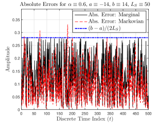
(a)

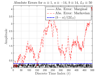
(b)

Figure 2: Absolute errors between each of the quantized versions of the $AR\left(1\right)$ process of our example, and the true process itself, respectively, for (a) $\alpha\equiv 0.6$ (stable process) and (b) $\alpha\equiv 1$ (a random walk).

Example 1.

Let $X_{t}$ be a scalar, first order autoregressive process ($AR\left(1\right)$), defined via the linear stochastic difference equation

$$X_{t}\triangleq\alpha X_{t-1}+W_{t},\quad\forall t\in\mathbb{N},$$ (17)

where $W_{t}\overset{i.i.d}{\sim}{\cal N}\left(0,1\right),\forall t\in\mathbb{N}$. In our example, the parameter $\alpha\in\left[-1,1\right]$ is known apriori and controls the stability of the process, with the case where $\alpha\equiv 1$ corresponding to a Gaussian random walk. Of course, it is true that the state space of the process defined by (17) is the whole $\mathbb{R}$, which means that, strictly speaking, there are no finite $a$ and $b$ such that $X_{t}\in\left[a,b\right]\equiv{\cal Z},\forall t\in\mathbb{N}$, with probability $1$. However, it is true that for sufficiently large but finite $a$ and $b$, there exists a “large” measurable set of possible outcomes for which $X_{t}$, being a Gaussian process, indeed belongs to ${\cal Z}$ with very high probability. Whenever this happens, we should be able to verify Lemmata 2 and 4 directly.

Additionally, it is trivial to verify that the linear transition function in (17) is always a contraction, with Lipschitz constant $K\equiv\left|\alpha\right|$, whenever the $AR\left(1\right)$ process of interest is stable, that is, whenever $\left|\alpha\right|<1$.

Fig. 2(a) and 2(b) show the absolute errors between two $AR\left(1\right)$ processes and their quantized versions according to Lemmata 2 and 4, for $\alpha\equiv 0.6$ and $\alpha\equiv 1$, respectively. From the figure, one can readily observe that the marginal quantization of $X_{t}$ always converges to $X_{t}$ uniformly in time, regardless of the particular value of $\alpha$, experimentally validating Lemma 2. On the other hand, it is obvious that when the transition function of our system is not a contraction (Lemma 4), uniform convergence of the respective Markovian quantization to the true state $X_{t}$ cannot be guaranteed. Of course, we have not proved any additional necessity regarding our sufficiency assumption related to the contractiveness of the transition mapping of the process of interest, meaning that there might exist processes which do not fulfill this requirement and still converge uniformly. However, for uniform contractions, the convergence will always be uniform whenever the process $X_{t}$ is bounded in ${\cal Z}$. $\blacksquare$

4 Grid Based Approximate Filtering:
Recursive Estimation & Asymptotic Optimality

It is indeed easy to show that when used as candidate state approximations for defining approximate filtering operators in the fashion of Section 2.B, both the marginal and Markovian quantization schemes presented in Sections 3.B and 3.C, respectively, converge to the optimal nonlinear filter of the state $X_{t}$. Convergence is in the sense of Theorem 1 presented in Section 2.B, corroborating asymptotic optimality under a unified convergence criterion.

Specifically, under the respective (and usual) assumptions, Lemmata 2 and 4 presented above imply that both the marginal and Markovian approximations converge to the true state $X_{t}$ at least in the almost sure sense, for all $t\in\mathbb{N}$. Therefore, both will also converge to the true state in probability, satisfying the second sufficient condition of Theorem 1. The following result is true. Its proof, being apparent, is omitted.

Theorem 2.

(Convergence of Approximate Filters) Pick any natural $T<\infty$ and let the process $X_{t}^{L_{S}}$ represent either the marginal or the Markovian approximation of the state $X_{t}$. Then, under the respective assumptions implied by Lemmata 2 and 4, the approximate filter ${\cal E}^{L_{S}}\left(\left.X_{t}\right|\mathscr{Y}_{t}\right)$ converges to the true nonlinear filter $\mathbb{E}_{{\cal P}}\left\{\left.X_{t}\right|\mathscr{Y}_{t}\right\}$, in the sense of Theorem 1.

Although Theorem 2 shows asymptotic consistency of the marginal and Markovian approximate filters in a strong sense, it does not imply the existence of any finite dimensional scheme for actually realizing these estimators. This is the purpose of the next subsections. In particular, we develop recursive representations for the asymptotically optimal (as $L_{S}\rightarrow\infty$) filter ${\cal E}^{L_{S}}\left(\left.X_{t}\right|\mathscr{Y}_{t}\right)$, as defined previously in (5).

For later reference, let us define the bijective mapping (a trivial quantizer) ${\cal Q}_{L_{S}}^{e}:\left({\cal X}_{L_{S}},2^{{\cal X}_{L_{S}}}\right)\mapsto\left({\cal V}_{L_{S}},2^{{\cal V}_{L_{S}}}\right)$, where the set ${\cal V}_{L_{S}}\triangleq\left\{{\bf e}_{1}^{L_{S}},\ldots,{\bf e}_{L_{S}}^{L_{S}}\right\}$ contains the complete standard basis in $\mathbb{R}^{L_{S}\times 1}$. Since $\boldsymbol{x}_{L_{S}}^{l}$ is bijectively mapped to ${\bf e}_{l}^{L_{S}}$ for all $l\in\mathbb{N}_{L_{S}}^{+}$, we can write $\boldsymbol{x}_{L_{S}}^{l}\equiv{\bf X}{\bf e}_{l}^{L_{S}}$, where ${\bf X}\triangleq\left[\boldsymbol{x}_{L_{S}}^{1}\,\boldsymbol{x}_{L_{S}}^{2}\,\ldots\,\boldsymbol{x}_{L_{S}}^{L_{S}}\right]\in\mathbb{R}^{M\times L_{S}}$ constitutes the respective reconstruction matrix. From this discussion, it is obvious that

$$\mathbb{E}_{\widetilde{{\cal P}}}\left\{\left.X_{t}^{L_{S}}\Lambda_{t}^{L_{S}}\right|\mathscr{Y}_{t}\right\}\equiv{\bf X}\mathbb{E}_{\widetilde{{\cal P}}}\left\{\left.{\cal Q}_{L_{S}}^{e}\left(X_{t}^{L_{S}}\right)\Lambda_{t}^{L_{S}}\right|\mathscr{Y}_{t}\right\},$$ (18)

leading to the expression

$${\cal E}^{L_{S}}\left(\left.X_{t}\right|\mathscr{Y}_{t}\right)\equiv\dfrac{{\bf X}\mathbb{E}_{\widetilde{{\cal P}}}\left\{\left.{\cal Q}_{L_{S}}^{e}\left(X_{t}^{L_{S}}\right)\Lambda_{t}^{L_{S}}\right|\mathscr{Y}_{t}\right\}}{\mathbb{E}_{\widetilde{{\cal P}}}\left\{\left.\Lambda_{t}^{L_{S}}\right|\mathscr{Y}_{t}\right\}},$$ (19)

for all $t\in\mathbb{N}$, regardless of the type of state quantization employed. We additionally define the likelihood matrix

$$\boldsymbol{\Lambda}_{t}\triangleq\mathrm{diag}\left(\mathsf{L}_{t}\left(\boldsymbol{x}_{L_{S}}^{1},{\bf y}_{t}\right)\,\ldots\,\mathsf{L}_{t}\left(\boldsymbol{x}_{L_{S}}^{L_{S}},{\bf y}_{t}\right)\right)\in\mathbb{R}^{L_{S}\times L_{S}}.$$ (20)

Also to be subsequently used, given the quantization type, define the column stochastic matrix $\boldsymbol{P}\in\left[0,1\right]^{L_{S}\times L_{S}}$ as

$$\boldsymbol{P}\left(i,j\right)\triangleq{\cal P}\left(\left.X_{t}^{L_{S}}\equiv\boldsymbol{x}_{L_{S}}^{i}\right|X_{t-1}^{L_{S}}\equiv\boldsymbol{x}_{L_{S}}^{j}\right),$$ (21)

for all $\left(i,j\right)\in\mathbb{N}_{L_{S}}^{+}\times\mathbb{N}_{L_{S}}^{+}$.

At this point, it will be important to note that the transition matrix $\boldsymbol{P}$ defined in (21) is implicitly assumed to be time invariant, regardless of the state approximation employed. Under the system model established in Section 2.A (assuming temporal homogeneity for the original Markov process $X_{t}$), this is unconditionally true when one considers Markovian state quantizations, simply because the resulting approximating process $X_{t}^{L_{S}}$ constitutes a Markov chain with finite state space, as stated earlier in Section 3.C. On the other hand, the situation is quite different when one considers marginal quantizations of the state. In that case, the conditional probabilities

$${\cal P}\left(\left.X_{t}^{L_{S}}\equiv\boldsymbol{x}_{L_{S}}^{i}\right|X_{t-1}^{L_{S}}\equiv\boldsymbol{x}_{L_{S}}^{j}\right) \equiv{\cal P}\left(\left.X_{t}\in{\cal Z}_{L_{S}}^{i}\right|X_{t-1}\in{\cal Z}_{L_{S}}^{j}\right),$$ (22)

which would correspond to the $\left(i,j\right)$-th element of the resulting transition matrix, are, in general, not time invariant any more, even if the original Markov process is time homogeneous. Nevertheless, assuming the existence of at least one invariant measure (a stationary distribution) for the Markov process $X_{t}$, also chosen as its initial distribution, the aforementioned probabilities are indeed time invariant. This is a very common and reasonable assumption employed in practice, especially when tracking stationary signals. For notational and intuitional simplicity, and in order to present a unified treatment of all the approximate filters considered in this paper, the aforementioned assumption will also be adopted in the analysis that follows.

4.1 Markovian Quantization

We start with the case of Markovian quantizations, since it is easier and more straightforward. Here, the development of the respective approximate filter is based on the fact that $X_{t}^{L_{S}}$ constitutes a Markov chain. Actually, this fact is the only requirement for the existence of a recursive realization of the filter, with Lemma 3 providing a sufficient condition, ensuring asymptotic optimality. The resulting recursive scheme is summarized in the following result. The proof is omitted, since it involves standard arguments in nonlinear filtering, similar to the ones employed in the derivation of the filtering recursions for a partially observed Markov chain with finite state space [3, 7, 38], as previously mentioned.

Theorem 3.

(The Markovian Filter) Consider the Markovian state approximation $X_{t}^{L_{S}}$ and define $\boldsymbol{E}_{t}\triangleq\mathbb{E}_{\widetilde{{\cal P}}}\left\{\left.{\cal Q}_{L_{S}}^{e}\left(X_{t}^{L_{S}}\right)\Lambda_{t}^{L_{S}}\right|\mathscr{Y}_{t}\right\}\in\mathbb{R}^{L_{S}\times 1}$, for all $t\in\mathbb{N}$. Then, under the appropriate assumptions (Lipschitz property of Lemma 4), the asymptotically optimal in $L_{S}$ approximate grid based filter ${\cal E}^{L_{S}}\left(\left.X_{t}\right|\mathscr{Y}_{t}\right)$ can be expressed as

$${\cal E}^{L_{S}}\left(\left.X_{t}\right|\mathscr{Y}_{t}\right)\equiv\dfrac{{\bf X}\boldsymbol{E}_{t}}{\left\|\boldsymbol{E}_{t}\right\|_{1}},\quad\forall t\in\mathbb{N},$$ (23)

where the process $\boldsymbol{E}_{t}$ satisfies the linear recursion

$$\boldsymbol{E}_{t}\equiv\boldsymbol{\Lambda}_{t}\boldsymbol{P}\boldsymbol{E}_{t-1},\quad\forall t\in\mathbb{N}.$$ (24)

The filter is initialized setting $\boldsymbol{E}_{-1}\triangleq\mathbb{E}_{{\cal P}}\left\{{\cal Q}_{L_{S}}^{e}\left(X_{-1}^{L_{S}}\right)\right\}$.

Remark 8.

It is worth mentioning that, although formally similar to, the approximate filter introduced in Theorem 3 does not refer to a Markov chain with finite state space, because the observations process utilized in the filtering iterations corresponds to that of the real partially observable system under consideration. The quantity ${\cal E}^{L_{S}}\left(\left.X_{t}\right|\mathscr{Y}_{t}\right)$ does not constitute a conditional expectation of the Markov chain associated with $\boldsymbol{P}$, because the latter process does not follow the probability law of the true state process $X_{t}$. $\blacksquare$

Remark 9.

In fact, $\boldsymbol{E}_{t}$ may be interpreted as a vector encoding an unnormalized point mass function, which, roughly speaking, expresses the belief of the quantized state, given the observations up to and including time $t$. Normalization by $\left\|\boldsymbol{E}_{t}\right\|_{1}$ corresponds precisely to a point mass function. $\blacksquare$

Remark 10.

For the benefit of the reader, we should mention that the Markovian filter considered above essentially coincides with the approximate grid based filter reported in ([24], Section IV.B), although the construction of the two filters is different: the former is constructed via a Markovian quantization of the state, whereas the latter [24] is based on a “quasi-marginal” approach (compare with (22)). Nevertheless, given our assumptions on the HMM under consideration, both formulations result in exactly the same transition matrix. Therefore, the optimality properties of the Markovian filter are indeed inherited by the grid based filter described in [24]. $\blacksquare$

4.2 Marginal Quantization

We now move on to the case of marginal quantizations. In order to be able to come up with a simple, Markov chain based, recursive filtering scheme, as in the case of Markovian quantizations previously treated, it turns out that a further assumption is required, this time concerning the stochastic kernel of the Markov process $X_{t}$. But before embarking on the relevant analysis, let us present some essential definitions.

First, for any process $X_{t}$, we will say that a sequence of functions $\left\{f_{n}\left(\cdot\right)\right\}_{n}$ is ${\cal P}_{X_{t}}-UI$, if $\left\{f_{n}\left(\cdot\right)\right\}_{n}$ is Uniformly Integrable with respect to the pushforward measure induced by $X_{t}$, ${\cal P}_{X_{t}}$, where $t\in\mathbb{N}\cup\left\{-1\right\}$, i.e.,

$$\lim_{K\rightarrow\infty}\sup_{n}\int_{\left\{\left|f_{n}\left(\boldsymbol{x}\right)\right|>K\right\}}\left|f_{n}\left(\boldsymbol{x}\right)\right|{\cal P}_{X_{t}}\left(\text{d}\boldsymbol{x}\right)\equiv 0.$$ (25)

Second, given $L_{S}$, recall from Section 3.A that the set $\Pi_{L_{S}}$ contains as members all quantization regions of ${\cal Z}$, ${\cal Z}_{L_{S}}^{j}$, $j\in\mathbb{N}_{L_{S}}^{+}$. Then, given the stochastic kernel ${\cal K}\left(\left.\cdot\right|\cdot\right)$ associated with the time invariant transitions of $X_{t}$ and for each $L_{S}\in\mathbb{N}^{+}$, we define the cumulative kernel

$${\cal K}\left(\left.{\cal A}\right|\in{\cal Z}_{L_{S}}\left(\boldsymbol{x}\right)\right) \triangleq\dfrac{{\displaystyle\int_{{\cal Z}_{L_{S}}\left(\boldsymbol{x}\right)}{\cal K}\left(\left.{\cal A}\right|\boldsymbol{\theta}\right){\cal P}_{X_{t-1}}\left(\text{d}\boldsymbol{\theta}\right)}}{{\cal P}\left(X_{t-1}\in{\cal Z}_{L_{S}}\left(\boldsymbol{x}\right)\right)}$$

$$\equiv\dfrac{\mathbb{E}\left\{{\cal K}\left(\left.{\cal A}\right|X_{t-1}\right)\mathds{1}_{\left\{X_{t-1}\in{\cal Z}_{L_{S}}\left(\boldsymbol{x}\right)\right\}}\right\}}{\mathbb{E}\left\{\mathds{1}_{\left\{X_{t-1}\in{\cal Z}_{L_{S}}\left(\boldsymbol{x}\right)\right\}}\right\}}$$

$$\equiv\mathbb{E}\left\{\left.{\cal K}\left(\left.{\cal A}\right|X_{t-1}\right)\right|X_{t-1}\in{\cal Z}_{L_{S}}\left(\boldsymbol{x}\right)\right\},$$ (26)

for all Borel ${\cal A}\in\mathscr{B}\left(\mathbb{R}^{M\times 1}\right)$ and all $\boldsymbol{x}\in{\cal Z}$, where ${\cal Z}_{L_{S}}\left(\boldsymbol{x}\right)\in\Pi_{L_{S}}$ denotes the unique quantization region, which includes $\boldsymbol{x}$. Note that if $\boldsymbol{x}$ is substituted by $X_{t-1}\left(\omega\right)$, the resulting quantity ${\cal Z}_{L_{S}}\left(X_{t-1}\left(\omega\right)\right)$ constitutes an $\mathscr{X}_{t}$-predictable set-valued random element. Now, if, for any $\boldsymbol{x}\in{\cal Z}$, ${\cal K}\left(\left.\cdot\right|\boldsymbol{x}\right)$ admits a stochastic kernel density $\kappa:\mathbb{R}^{M\times 1}\times\mathbb{R}^{M\times 1}\mapsto\mathbb{R}_{+},$ suggestively denoted as $\kappa\left(\left.\boldsymbol{y}\right|\boldsymbol{x}\right)$, we define, in exactly the same fashion as above, the cumulative kernel density

$$\kappa\left(\left.\boldsymbol{y}\right|\in{\cal Z}_{L_{S}}\left(\boldsymbol{x}\right)\right)\triangleq\mathbb{E}\left\{\left.\kappa\left(\left.\boldsymbol{y}\right|X_{t-1}\right)\right|X_{t-1}\in{\cal Z}_{L_{S}}\left(\boldsymbol{x}\right)\right\},$$ (27)

for all $\boldsymbol{y}\in\mathbb{R}^{M\times 1}$. The fact that $\kappa\left(\left.\cdot\right|\in{\cal Z}_{L_{S}}\left(\boldsymbol{x}\right)\right)$ is indeed a Radon-Nikodym derivative of ${\cal K}\left(\left.\cdot\right|\in{\cal Z}_{L_{S}}\left(\boldsymbol{x}\right)\right)$ readily follows by definition of the latter and Fubini’s Theorem.

Remark 11.

Observe that, although integration is with respect to ${\cal P}_{X_{t-1}}$ on the RHS of (26), ${\cal K}\left(\left.\cdot\right|\in{\cal Z}_{L_{S}}\left(\cdot\right)\right)$ is time invariant. This is due to stationarity of $X_{t}$, as assumed in the beginning of Section 4, implying time invariance of the marginal measure ${\cal P}_{X_{t}}$, for all $t\in\mathbb{N}\cup\left\{-1\right\}$. Additionally, for each $\boldsymbol{x}\in{\cal Z}$, when ${\cal A}$ is restricted to $\Pi_{L_{S}}$, ${\cal K}\left(\left.{\cal A}\right|\in{\cal Z}_{L_{S}}\left(\boldsymbol{x}\right)\right)$ corresponds to an entry of the (time invariant) matrix $\boldsymbol{P}$, also defined earlier. In the general case, where the aforementioned cumulative kernel is time varying, all subsequent analysis continues to be valid, just by adding additional notational complexity. $\blacksquare$

In respect to the relevant assumption required on ${\cal K}\left(\left.\cdot\right|\cdot\right)$, as asserted above, let us now present the following definition.

Definition 2.

(Cumulative Conditional Regularity of Markov Kernels) Consider the kernel ${\cal K}\left(\left.\cdot\right|\cdot\right)$, associated with $X_{t}$, for all $t\in\mathbb{N}$. We say that ${\cal K}\left(\left.\cdot\right|\cdot\right)$ is Conditionally Regular of Type I (CRT I), if, for ${\cal P}_{X_{t}}\equiv{\cal P}_{X_{-1}}$-almost all $\boldsymbol{x}$, there exists a ${\cal P}_{X_{-1}}-UI$ sequence $\left\{\delta_{n}^{I}\left(\cdot\right)\geq 0\right\}_{n\in\mathbb{N}^{+}}$ with $\delta_{n}^{I}\left(\cdot\right)\stackrel{{\scriptstyle[}}{{n}}\rightarrow\infty]{a.e.}{\longrightarrow}0$, such that

$${\displaystyle\sup_{{\cal A}\in\Pi_{L_{S}}}}\left|{\cal K}\left(\left.{\cal A}\right|\boldsymbol{x}\right)-{\cal K}\left(\left.{\cal A}\right|\in{\cal Z}_{L_{S}}\left(\boldsymbol{x}\right)\right)\right|\leq\dfrac{\delta_{L_{S}}^{I}\left(\boldsymbol{x}\right)}{L_{S}}.$$ (28)

If, further, for ${\cal P}_{X_{-1}}$-almost all $\boldsymbol{x}$, the measure ${\cal K}\left(\left.\cdot\right|\boldsymbol{x}\right)$ admits a density $\kappa\left(\left.\cdot\right|\boldsymbol{x}\right),$ and if there exists another ${\cal P}_{X_{-1}}-UI$ sequence $\left\{\delta_{n}^{II}\left(\cdot\right)\geq 0\right\}_{n\in\mathbb{N}^{+}}$ with $\delta_{n}^{II}\left(\cdot\right)\stackrel{{\scriptstyle[}}{{n}}\rightarrow\infty]{a.e.}{\longrightarrow}0$, such that

$$\underset{\boldsymbol{y}\in\mathbb{R}^{M\times 1}}{\mathrm{ess}\hskip 1.99997pt\mathrm{sup}}\left|\kappa\left(\left.\boldsymbol{y}\right|\boldsymbol{x}\right)-\kappa\left(\left.\boldsymbol{y}\right|\in{\cal Z}_{L_{S}}\left(\boldsymbol{x}\right)\right)\right|\leq\delta_{L_{S}}^{II}\left(\boldsymbol{x}\right),$$ (29)

${\cal K}\left(\left.\cdot\right|\cdot\right)$ is called Conditionally Regular of Type II (CRT II). In any case, $X_{t}$ will also be called conditionally regular.

 

A consequence of conditional regularity is the following Martingale Difference (MD) [6, 7] type representation of the marginally quantized process ${\cal Q}_{L_{S}}^{e}\left(X_{t}^{L_{S}}\right)$.

Lemma 5.

(Semirecursive MD-type Representation of Marginal Quantizations) Assume that the state process $X_{t}$ is conditionally regular. Then, the quantized process ${\cal Q}_{L_{S}}^{e}\left(X_{t}^{L_{S}}\right)$ admits the representation

$${\cal Q}_{L_{S}}^{e}\left(X_{t}^{L_{S}}\right) \equiv\boldsymbol{P}{\cal Q}_{L_{S}}^{e}\left(X_{t-1}^{L_{S}}\right)+\boldsymbol{{\cal M}}_{t}^{e}+\boldsymbol{\varepsilon}_{t}^{L_{S}},$$ (30)

where, under the base measure $\widetilde{{\cal P}}$,$\boldsymbol{{\cal M}}_{t}^{e}\in\mathbb{R}^{L_{S}\times 1}$ constitutes an $\mathscr{X}_{t}$-MD process and $\boldsymbol{\varepsilon}_{t}^{L_{S}}\in\mathbb{R}^{L_{S}\times 1}$ constitutes a $\left\{\mathscr{X}_{t}\right\}$-predictable process, such that

• if $X_{t}$ is CRT I, then

  $$\left\|\boldsymbol{\varepsilon}_{t}^{L_{S}}\right\|_{1}\leq\delta_{L_{S}}^{I}\left(X_{t-1}\right)\underset{L_{S}\rightarrow\infty}{\longrightarrow}0,\;\widetilde{{\cal P}}-a.s.,$$ (31)

• whereas, if $X_{t}$ is CRT II, then

  $$\left\|\boldsymbol{\varepsilon}_{t}^{L_{S}}\right\|_{1}\leq\left|b-a\right|^{M}\delta_{L_{S}}^{II}\left(X_{t-1}\right)\underset{L_{S}\rightarrow\infty}{\longrightarrow}0,\;\widetilde{{\cal P}}-a.s.,$$ (32)

everywhere in time.

Proof of Lemma 5.

See Appendix B. ∎

Now, consider an auxiliary Markov chain $Z_{t}^{L_{S}}\in{\cal V}_{L_{S}}$, with $\boldsymbol{P}$ (defined as in (21)) as its transition matrix and with initial distribution to be specified. Of course, $Z_{t}^{L_{S}}$ can be represented as $Z_{t}^{L_{S}}\equiv\boldsymbol{P}Z_{t-1}^{L_{S}}+\widetilde{\boldsymbol{{\cal M}}}_{t}^{e}$, where $\widetilde{\boldsymbol{{\cal M}}}_{t}^{e}\in\mathbb{R}^{L_{S}\times 1}$ constitutes a $\mathscr{Z}_{t}$-MD process, with $\left\{\mathscr{Z}_{t}\right\}_{t\in\mathbb{N}}$ being the complete natural filtration generated by $Z_{t}^{L_{S}}$.

Due to the existence of the “bias” process $\boldsymbol{\varepsilon}_{t}^{L_{S}}$ in the martingale difference representation of ${\cal Q}_{L_{S}}^{e}\left(X_{t}^{L_{S}}\right)$ (see Lemma 5), the direct derivation of a filtering recursion for this process is difficult. However, it turns out that the approximate filter involving the marginal state quantization $X_{t}^{L_{S}}$, ${\cal E}^{L_{S}}\left(\left.X_{t}\right|\mathscr{Y}_{t}\right)$, can be further approximated by the also approximate filter

$$\widetilde{{\cal E}}^{L_{S}}\left(\left.X_{t}\right|\mathscr{Y}_{t}\right)\triangleq\dfrac{{\bf X}\mathbb{E}_{\widetilde{{\cal P}}}\left\{\left.Z_{t}^{L_{S}}\Lambda_{t}^{Z,L_{S}}\right|\mathscr{Y}_{t}\right\}}{\mathbb{E}_{\widetilde{{\cal P}}}\left\{\left.\Lambda_{t}^{Z,L_{S}}\right|\mathscr{Y}_{t}\right\}},$$ (33)

for all $t\in\mathbb{N}$, where the functional $\Lambda_{t}^{Z,L_{S}}$ is defined exactly like $\Lambda_{t}^{L_{S}},$ but replacing $X_{t}^{L_{S}}$ with $Z_{t}^{L_{S}}$. This latter filter indeed admits the recursive representation proposed in Theorem 3 (with $\boldsymbol{P}$ defined as in (21), reflecting the choice of a marginal state approximation).

Consequently, if we are interested in the asymptotic behavior of the approximation error between $\widetilde{{\cal E}}^{L_{S}}\left(\left.X_{t}\right|\mathscr{Y}_{t}\right)$ and the original nonlinear filter $\mathbb{E}_{{\cal P}}\left\{\left.X_{t}\right|\mathscr{Y}_{t}\right\}$, we can write

$$\left\|\mathbb{E}_{{\cal P}}\left\{\left.X_{t}\right|\mathscr{Y}_{t}\right\}-\widetilde{{\cal E}}^{L_{S}}\left(\left.X_{t}\right|\mathscr{Y}_{t}\right)\right\|_{1}\\ \leq\left\|\mathbb{E}_{{\cal P}}\left\{\left.X_{t}\right|\mathscr{Y}_{t}\right\}-{\cal E}^{L_{S}}\left(\left.X_{t}\right|\mathscr{Y}_{t}\right)\right\|_{1}+\left\|{\cal E}^{L_{S}}\left(\left.X_{t}\right|\mathscr{Y}_{t}\right)-\widetilde{{\cal E}}^{L_{S}}\left(\left.X_{t}\right|\mathscr{Y}_{t}\right)\right\|_{1}.$$ (34)

However, from Theorem 2, we know that, under the respective conditions,

$$\sup_{t\in\mathbb{N}_{T}}\sup_{\omega\in\widehat{\Omega}_{T}}\left\|{\cal E}^{L_{S}}\left(\left.X_{t}\right|\mathscr{Y}_{t}\right)-\mathbb{E}_{{\cal P}}\left\{\left.X_{t}\right|\mathscr{Y}_{t}\right\}\right\|_{1}\underset{L_{S}\rightarrow\infty}{\longrightarrow}0.$$ (35)

Therefore, if we show that error between ${\cal E}^{L_{S}}\left(\left.X_{t}\right|\mathscr{Y}_{t}\right)$ and $\widetilde{{\cal E}}^{L_{S}}\left(\left.X_{t}\right|\mathscr{Y}_{t}\right)$ vanishes in the above sense, then, $\widetilde{{\cal E}}^{L_{S}}\left(\left.X_{t}\right|\mathscr{Y}_{t}\right)$ will converge to $\mathbb{E}_{{\cal P}}\left\{\left.X_{t}\right|\mathscr{Y}_{t}\right\}$, also in the same sense. It turns out that if $X_{t}$ is conditionally regular, the aforementioned desired statement always holds, as follows.

Lemma 6.

(Convergence of Approximate Filters) For any natural $T<\infty$, suppose that the state process $X_{t}$ is conditionally regular and that the initial measure of the chain $Z_{t}^{L_{S}}$ is chosen such that

$$\mathbb{E}_{\widetilde{{\cal P}}}\left\{Z_{-1}^{L_{S}}\right\}\equiv\mathbb{E}_{{\cal P}}\left\{{\cal Q}_{L_{S}}^{e}\left(X_{-1}^{L_{S}}\right)\right\}.$$ (36)

Then, for the same measurable subset $\widehat{\Omega}_{T}\subseteq\Omega$ of Theorem 1, it is true that

$$\sup_{t\in\mathbb{N}_{T}}\sup_{\omega\in\widehat{\Omega}_{T}}\left\|{\cal E}^{L_{S}}\left(\left.X_{t}\right|\mathscr{Y}_{t}\right)-\widetilde{{\cal E}}^{L_{S}}\left(\left.X_{t}\right|\mathscr{Y}_{t}\right)\right\|_{1}\underset{L_{S}\rightarrow\infty}{\longrightarrow}0.$$ (37)

Additionally, under the same setting, it follows that

$$\sup_{t\in\mathbb{N}_{T}}\sup_{\omega\in\widehat{\Omega}_{T}}\left\|\widetilde{{\cal E}}^{L_{S}}\left(\left.X_{t}\right|\mathscr{Y}_{t}\right)-\mathbb{E}_{{\cal P}}\left\{\left.X_{t}\right|\mathscr{Y}_{t}\right\}\right\|_{1}\underset{L_{S}\rightarrow\infty}{\longrightarrow}0.$$ (38)

Proof of Lemma 6.

See Appendix C. ∎

Finally, the next theorem establishes precisely the form of the recursive grid based filter, employing the marginal quantization of the state.

Theorem 4.

(The Marginal Filter) Consider the marginal state approximation $X_{t}^{L_{S}}$ and suppose that the state process $X_{t}$ is conditionally regular. Then, for each $t\in\mathbb{N}$, the asymptotically optimal in $L_{S}$ approximate filtering operator $\widetilde{{\cal E}}^{L_{S}}\left(\left.X_{t}\right|\mathscr{Y}_{t}\right)$ can be recursively expressed exactly as in Theorem 3, with initial conditions as in Lemma 6 and transition matrix $\boldsymbol{P}$ defined as in (21).

Remark 12.

(Weak Conditional Regularity) All the derivations presented above are still valid if, in the definition of conditional regularity (Definition 2), one replaces almost everywhere convergence of the sequences $\left\{\delta_{n}^{I}\left(\cdot\right)\right\}_{n}$ and $\left\{\delta_{n}^{II}\left(\cdot\right)\right\}_{n}$ with convergence in probability. This is due to the fact that uniform integrability plus convergence in measure are necessary and sufficient conditions for showing convergence in ${\cal L}_{1}$ (for finite measure spaces). Consequently, if we focus on, for instance, CRT I (CRT II is similar), it is easy to see that in order to ensure asymptotic consistency of the marginal approximate filter in the sense of Theorem 4, it suffices that, for ${\cal A}\in\Pi_{L_{S}}$ and for any $\epsilon>0$,

$${\cal P}_{X_{t-1}}\left(\sup_{{\cal A}}\left|{\cal K}\left(\left.{\cal A}\right|\boldsymbol{x}\right)-{\cal K}\left(\left.{\cal A}\right|\in{\cal Z}_{L_{S}}\left(\boldsymbol{x}\right)\right)\right|>\dfrac{\epsilon}{L_{S}}\right)\underset{L_{S}\rightarrow\infty}{\longrightarrow}0,$$ (39)

for all $t\in\mathbb{N}$ (in general), given the stochastic kernel ${\cal K}\left(\left.\cdot\right|\cdot\right)$ and for the desired choice of the quantizer ${\cal Q}_{L_{S}}\left(\cdot\right)$. Here, the ${\cal P}_{X_{t}}-UI$ sequence $\left\{\delta_{n}^{I}\left(\cdot\right)\right\}_{n}$ is identified as

$$\delta_{L_{S}}^{I}\left(\boldsymbol{x}\right)\equiv\sup_{{\cal A}\in\Pi_{L_{S}}}L_{S}\left|{\cal K}\left(\left.{\cal A}\right|\boldsymbol{x}\right)-{\cal K}\left(\left.{\cal A}\right|\in{\cal Z}_{L_{S}}\left(\boldsymbol{x}\right)\right)\right|,$$ (40)

for all $L_{S}\in\mathbb{N}^{+}$ and for almost all $\boldsymbol{x}\in\mathbb{R}^{M\times 1}$. In other words, it is required that, for any $\epsilon>0$,

$$\sup_{{\cal A}\in\Pi_{L_{S}}}\left|{\cal K}\left(\left.{\cal A}\right|X_{t-1}\right)-{\cal K}\left(\left.{\cal A}\right|\in{\cal Z}_{L_{S}}\left(X_{t-1}\right)\right)\right|\leq\dfrac{\epsilon}{L_{S}},$$ (41)

with probability at least $1-\pi_{t-1}\left(\epsilon,L_{S}\right)$, for all $t\in\mathbb{N}$ (in general), where, for each $t,$ $\left\{\pi_{t-1}\left(\epsilon,n\right)\right\}_{n\in\mathbb{N}^{+}}$ constitutes a sequence vanishing at infinity. This is a considerably weaker form of conditional regularity, as stated in Definition 2. $\blacksquare$

4.3 Extensions: State Functionals & Approximate Prediction

All the results presented so far can be extended as follows. First, if $\left\{\boldsymbol{\phi}_{t}:\mathbb{R}^{M\times 1}\mapsto\mathbb{R}^{M_{\phi_{t}}\times 1}\right\}_{t\in\mathbb{N}}$ is a family of bounded and continuous functions, it is easy to show that every relevant theorem presented so far is still true if one replaces $X_{t}$ by $\boldsymbol{\phi}_{t}\left(X_{t}\right)$ in the respective formulations of the approximate filters discussed. This is made possible by observing that (4) still holds if we replace $X_{t}$ by $\boldsymbol{\phi}_{t}\left(X_{t}\right)$, by invoking the Continuous Mapping Theorem and using the boundedness of $\boldsymbol{\phi}_{t}\left(X_{t}\right)$, instead of the boundedness of $X_{t}$, whenever required.

Second, exploiting very similar arguments as in the previous sections, it is possible to derive asymptotically optimal $\rho$-step state predictors, where $\rho>0$ denotes the desired (and finite) prediction horizon. In particular, under the usual assumptions [7], it is easy to show that, as in the filtering case, the optimal nonlinear temporal predictor $\mathbb{E}_{{\cal P}}\left\{\left.X_{t+\rho}\right|\mathscr{Y}_{t}\right\}$ can be expressed through the Feynman-Kac type of formula

$$\mathbb{E}_{{\cal P}}\left\{\left.X_{t+\rho}\right|\mathscr{Y}_{t}\right\}\equiv\dfrac{\mathbb{E}_{\widetilde{{\cal P}}}\left\{\left.X_{t+\rho}\Lambda_{t}\right|\mathscr{Y}_{t}\right\}}{\mathbb{E}_{\widetilde{{\cal P}}}\left\{\left.\Lambda_{t}\right|\mathscr{Y}_{t}\right\}},\quad\forall t\in\mathbb{N}.$$ (42)

Therefore, in analogy to (19), it is reasonable to consider grid based approximations of the form

$${\cal E}^{L_{S}}\left(\left.X_{t+\rho}\right|\mathscr{Y}_{t}\right)\equiv\dfrac{{\bf X}\mathbb{E}_{\widetilde{{\cal P}}}\left\{\left.{\cal Q}_{L_{S}}^{e}\left(X_{t+\rho}^{L_{S}}\right)\Lambda_{t}^{L_{S}}\right|\mathscr{Y}_{t}\right\}}{\mathbb{E}_{\widetilde{{\cal P}}}\left\{\left.\Lambda_{t}^{L_{S}}\right|\mathscr{Y}_{t}\right\}},$$ (43)

for all $t\in\mathbb{N}$. Focusing on marginal state quantizations (the Markovian case is similar, albeit easier), then, exploiting Lemma 5 and using induction, it is easy to show that

$${\cal Q}_{L_{S}}^{e}\left(X_{t+\rho}^{L_{S}}\right) \equiv\boldsymbol{P}^{\rho}{\cal Q}_{L_{S}}^{e}\left(X_{t}^{L_{S}}\right)+\sum_{i=1}^{\rho}\boldsymbol{P}^{\rho-i}\boldsymbol{{\cal M}}_{t+i}^{e}+\sum_{i=1}^{\rho}\boldsymbol{P}^{\rho-i}\boldsymbol{\varepsilon}_{t+i}^{L_{S}},\quad\forall t\in\mathbb{N}.$$ (44)

Thus, using simple properties of MD sequences, it follows that the numerator of the fraction on the RHS of (43) can be decomposed as

$${\cal E}^{L_{S}}\left(\left.X_{t+\rho}\right|\mathscr{Y}_{t}\right) \equiv\dfrac{{\bf X}\boldsymbol{P}^{\rho}\mathbb{E}_{\widetilde{{\cal P}}}\left\{\left.{\cal Q}_{L_{S}}^{e}\left(X_{t+\rho}^{L_{S}}\right)\Lambda_{t}^{L_{S}}\right|\mathscr{Y}_{t}\right\}}{\mathbb{E}_{\widetilde{{\cal P}}}\left\{\left.\Lambda_{t}^{L_{S}}\right|\mathscr{Y}_{t}\right\}}+\dfrac{{\displaystyle{\bf X}\sum_{i=1}^{\rho}\boldsymbol{P}^{\rho-i}\mathbb{E}_{\widetilde{{\cal P}}}\left\{\left.\boldsymbol{\varepsilon}_{t+i}^{L_{S}}\Lambda_{t}^{L_{S}}\right|\mathscr{Y}_{t}\right\}}}{\mathbb{E}_{\widetilde{{\cal P}}}\left\{\left.\Lambda_{t}^{L_{S}}\right|\mathscr{Y}_{t}\right\}}.$$ (45)

The first term on the RHS of (45) is analyzed exactly as in the proof of Lemma 6. For the second term, it is true that

$$\left\|{\displaystyle{\bf X}\sum_{i=1}^{\rho}\boldsymbol{P}^{\rho-i}\mathbb{E}_{\widetilde{{\cal P}}}\left\{\left.\boldsymbol{\varepsilon}_{t+i}^{L_{S}}\Lambda_{t}^{L_{S}}\right|\mathscr{Y}_{t}\right\}}\right\|_{1} \leq M\gamma\sqrt{\lambda_{inf}^{-N\left(t+1\right)}}\sum_{i=1}^{\rho}\mathbb{E}_{\widetilde{{\cal P}}}\left\{\left\|\boldsymbol{\varepsilon}_{t+i}^{L_{S}}\right\|_{1}\right\},$$ (46)

which can be treated as an extra error term, also in the fashion of Lemma 6.

Putting it altogether (state functionals plus prediction), the following general theorem holds, covering every aspect of the investigation presented in this paper.

Theorem 5.

(Grid Based Filtering/Prediction & Functionals of the State) For any deterministic functional family $\left\{\boldsymbol{\phi}_{t}:\mathbb{R}^{M\times 1}\mapsto\mathbb{R}^{M_{\phi_{t}}\times 1}\right\}_{t\in\mathbb{N}}$ with bounded and continuous members and any finite prediction horizon $\rho\geq 0$, the strictly optimal filter and $\rho$-step predictor of the transformed process $\boldsymbol{\phi}_{t}\left(X_{t}\right)$ can be approximated as

$${\cal E}^{L_{S}}\left(\left.\boldsymbol{\phi}_{t+\rho}\left(X_{t+\rho}\right)\right|\mathscr{Y}_{t}\right)\triangleq\boldsymbol{\Phi}_{t+\rho}\dfrac{\boldsymbol{P}^{\rho}\boldsymbol{E}_{t}}{\left\|\boldsymbol{E}_{t}\right\|_{1}}\in\mathbb{R}^{M_{\phi_{t}}\times 1},$$ (47)

for all $t\in\mathbb{N}$, where the process $E_{t}\in\mathbb{R}^{L_{S}\times 1}$ can be recursively evaluated as in Theorem 3, $\boldsymbol{P}$ is defined according to the chosen state quantization and

$$\boldsymbol{\Phi}_{t+\rho}\triangleq\left[\boldsymbol{\phi}_{t+\rho}\left(\boldsymbol{x}_{L_{S}}^{1}\right)\,\ldots\,\boldsymbol{\phi}_{t+\rho}\left(\boldsymbol{x}_{L_{S}}^{L_{S}}\right)\right]\in\mathbb{R}^{M_{\phi_{t}}\times L_{S}}.$$ (48)

Additionally, under the appropriate assumptions (see Lemma 4 and Lemma 6, respectively) the approximate filter is asymptotically optimal. in the sense of Theorem 1.

Remark 13.

As Theorem 5 clearly states, for each choice of state functionals and any finite prediction horizon, convergence of the respective approximate grid based filters is in the sense of Theorem 1. This implies the existence of an exceptional measurable set of measure almost unity, inside of which convergence is in the uniform sense. It is important to emphasize that this exceptional event, $\widehat{\Omega}_{T}$, as well as its measure, are independent of the particular choice of both the bounded family $\left\{\boldsymbol{\phi}_{t}\right\}_{t}$ and the prediction horizon $\rho$. This fact can be easily verified by a quick detour of the proof of Theorem 1 in [31]. In particular, for any fixed choice of $T$, $\widehat{\Omega}_{T}$ characterizes exclusively the growth of the observations ${\bf y}_{t}$, which are the same regardless of filtering, prediction, or any functional imposed on the state. Therefore, stochastically uniform (in $\widehat{\Omega}_{T}$) convergence of one estimator implies stochastically uniform convergence of any other estimator, within any class of estimators, constructed employing any uniformly bounded and continuous class of functionals of the state and finite prediction horizons. $\blacksquare$

4.4 Filter Performance

The uncertainty of a filtering estimator can be quantified via its posterior quadratic deviation from the true state, at each time $t$. This information is encoded into the posterior covariance matrix

$$\mathbb{V}\left\{\left.X_{t}\right|\mathscr{Y}_{t}\right\}\equiv\mathbb{E}\left\{\left.X_{t}X_{t}^{\boldsymbol{T}}\right|\mathscr{Y}_{t}\right\}-\mathbb{E}\left\{\left.X_{t}\right|\mathscr{Y}_{t}\right\}\left(\mathbb{E}\left\{\left.X_{t}\right|\mathscr{Y}_{t}\right\}\right)^{\boldsymbol{T}},$$ (49)

for all $t\in\mathbb{N}$. Next, in a general setting, we consider asymptotically consistent approximations of $\mathbb{V}\left\{\left.\boldsymbol{\phi}_{t+\rho}\left(X_{t+\rho}\right)\right|\mathscr{Y}_{t}\right\}$, which, at the same time, admit finite dimensional representations. In the following, $\left\|\cdot\right\|_{1}^{\mathsf{E}}$ denotes the entrywise $\ell_{1}$-norm for matrices, which upper bounds both the $\ell_{1}$-operator-induced and the Frobenius norms.

Theorem 6.

(Posterior Covariance Recursions) Under the same setting as in Theorem 5, the posterior covariance matrix of the optimal filter of the transformed process $\boldsymbol{\phi}_{t+\rho}\left(X_{t+\rho}\right)$ can be approximated as

$${\cal V}^{L_{S}}\left(\left.\boldsymbol{\phi}_{t+\rho}\left(X_{t+\rho}\right)\right|\mathscr{Y}_{t}\right) \triangleq\boldsymbol{\Phi}_{t+\rho}\mbox{$\left[\mathrm{diag}\left(\dfrac{\boldsymbol{P}^{\rho}\boldsymbol{E}_{t}}{\left\|\boldsymbol{E}_{t}\right\|_{1}}\right)-\dfrac{\boldsymbol{P}^{\rho}\boldsymbol{E}_{t}}{\left\|\boldsymbol{E}_{t}\right\|_{1}}\left(\dfrac{\boldsymbol{P}^{\rho}\boldsymbol{E}_{t}}{\left\|\boldsymbol{E}_{t}\right\|_{1}}\right)^{\boldsymbol{T}}\right]$}\boldsymbol{\Phi}_{t+\rho}^{\boldsymbol{T}},$$ (50)

for all $t\in\mathbb{N}$. Under the appropriate assumptions (Lemma 4/6), the approximate estimator is asymptotically optimal in the sense of Theorem 1.

Proof of Theorem 6.

See Appendix D. ∎

5 Analytical Examples & Some Simulations

This section is centered around a discussion about the practical applicability of the grid based filters under consideration, mainly in regard to filter implementation, as well as the sufficient conditions for asymptotic optimality presented and analyzed in Section 4. In what follows, we consider a class of $1$-dimensional (for simplicity), common and rather practically important additive Nonlinear AutoRegressions (NARs), where $X_{t}$ evolves according to the stochastic difference equation

$$X_{t}\equiv h\left(X_{t-1}\right)+W_{t},\quad\forall t\in\mathbb{N},$$ (51)

$X_{-1}\sim{\cal P}_{X_{-1}}$, where $h\left(\cdot\right)$ constitutes a uniformly bounded and at least continuous nonlinear functional and $W_{t}$ is a white noise process with known measure. To ensure that the state is bounded, we will assume that the white noise $W_{t}$ follows, for each $t\in\mathbb{N}$, a zero location (and mean), truncated Gaussian distribution in $\left[-\alpha,\alpha\right]$, with scale $\sigma$ and with density

$$f_{W}\left(x\right)\triangleq\dfrac{\varphi\left(x/\sigma\right)}{2\sigma\varPhi\left(\alpha/\sigma\right)-\sigma}\mathds{1}_{\left[-\alpha,\alpha\right]}\left(x\right),\;\forall x\in\mathbb{R},$$ (52)

where $\varphi\left(\cdot\right)$ and $\varPhi\left(\cdot\right)$ denote the standard Gaussian density and cumulative distribution functions, respectively. Under these considerations, if $\sup_{x\in\mathbb{R}}\left|h\left(x\right)\right|\equiv B$, then $\left|X_{t}\right|\leq B+\alpha$ and, thus, ${\cal Z}$ is identified as the set $\left[a,b\equiv-a\right]$, with $b\triangleq B+\alpha$.

5.1 Markovian Filter

In this case, the respective approximation of the state process is given by the quantized stochastic difference equation

$$X_{t}^{L_{S}}\triangleq{\cal Q}_{L_{S}}\left(h\left(X_{t-1}^{L_{S}}\right)+W_{t}\right),\quad\forall t\in\mathbb{N},$$ (53)

initialized as $X_{-1}^{L_{S}}\equiv{\cal Q}_{L_{S}}\left(X_{-1}\right)$, with probability $1$. In order to guarantee asymptotic optimality of the respective approximate filter described in Theorem 3, the original process $X_{t}$ is required to at least satisfy the basic Lipschitz condition of Assumption 3. Indeed, if we merely assume that $h\left(\cdot\right)$ is additionally Lipschitz with constant $L_{h}>0$ (that is, regardless of the stochastic character of $W_{t}$, in general), then the function

$$f\left(x,y\right)\triangleq h\left(x\right)+y,\quad\left(x,y\right)\in\left[-B,B\right]\times\left[-\alpha,\alpha\right]$$ (54)

is also Lipschitz with respect to $x$ (for all $y$), with constant $L_{h}$ as well. Therefore, under the mild Lipschitz assumption for $h\left(\cdot\right)$, we have shown that the resulting Markovian filter will indeed be asymptotically consistent. In practice, we expect that a smaller constant $L_{h}$ would result in better performance of the approximate filter, with best results if $h\left(\cdot\right)$ constitutes a contraction, which makes $f\left(\cdot,y\right)$ uniformly contractive in $y$. The above is indeed true, since filtering is essentially implemented via a stochastic difference equation itself, and, in general, any discretized approximation to this difference equation is subject to error accumulation.

Of course, in order for the Markovian filter to be realizable, both the transition matrix $\boldsymbol{P}$ and the initial value $\boldsymbol{E}_{-1}$ have to be determined. In all cases, under our assumptions, $\boldsymbol{P}$ (and obviously $\boldsymbol{E}_{-1}$) may be determined during an offline training phase, and stored in memory. A brute force way for estimating $\boldsymbol{P}$ is to simulate $X_{t}$ (recall that the stochastic description of the transitions of $X_{t}$ is known apriori). Then, $\boldsymbol{P}$ can be empirically estimated using the Strong Law of Large Numbers (SLLN). The aforementioned procedure results in excellent performance in practice [13]. Exactly the same idea may be employed in order to estimate $\boldsymbol{E}_{-1}$, given the initial measure of $X_{t}$. Note that the above described empirical method for the estimation of $\boldsymbol{P}$ and $\boldsymbol{E}_{-1}$ does not assume a specific model describing the temporal evolution of $X_{t}$, or any particular choice of state quantization. Thus, it is generally applicable.

However, for the specific (though general) class of systems discussed above, we may also present an analytical construction for $\boldsymbol{P}$ (and $\boldsymbol{E}_{-1}$, assuming ${\cal P}_{X_{-1}}$ is known), resulting in compact, closed form expressions. Indeed, by definition of $X_{t}^{L_{S}}$, $\boldsymbol{P}\left(i,j\right)$ and each ${\cal Z}_{L_{S}}^{i}$, whose center is $\boldsymbol{x}_{L_{S}}^{i}$, we get

$$\boldsymbol{P}\left(i,j\right) \equiv{\cal P}\left(\left.h\left(X_{t-1}^{L_{S}}\right)+W_{t}\in{\cal Z}_{L_{S}}^{i}\right|X_{t-1}^{L_{S}}\equiv\boldsymbol{x}_{L_{S}}^{j}\right)$$

$$=\int_{{\cal Z}_{L_{S}}^{i}}f_{W}\left(x-h\left(\boldsymbol{x}_{L_{S}}^{j}\right)\right)\mathrm{d}x,$$ (55)

which, based on (51), can be written in closed form as

$$\boldsymbol{P}\left(i,j\right)\equiv\dfrac{\varPhi\left(\dfrac{p_{L_{S}}^{ij}\left(\alpha,B\right)}{\sigma}\right)-\varPhi\left(\dfrac{q_{L_{S}}^{ij}\left(\alpha,B\right)}{\sigma}\right)}{2\sigma\varPhi\left(\alpha/\sigma\right)-\sigma}\mathds{1}_{\left(-\infty,p\right)}\left(q\right),$$ (56)

for all $\left(i,j\right)\in\mathbb{N}_{L_{S}}^{+}\times\mathbb{N}_{L_{S}}^{+}$, where

$$p_{L_{S}}^{ij}\left(\alpha,B\right) \triangleq\min\left\{\alpha,\boldsymbol{x}_{L_{S}}^{i}-h\left(\boldsymbol{x}_{L_{S}}^{j}\right)+\dfrac{B+\alpha}{L_{S}}\right\}\;\text{and}$$ (57)

$$q_{L_{S}}^{ij}\left(\alpha,B\right) \triangleq\max\left\{-\alpha,\boldsymbol{x}_{L_{S}}^{i}-h\left(\boldsymbol{x}_{L_{S}}^{j}\right)-\dfrac{B+\alpha}{L_{S}}\right\}.$$ (58)

Consequently, via (56), one may obtain the whole matrix $\boldsymbol{P}$ for any set of parameters $\sigma,\alpha,B$ and for any resolution $L_{S}$. As far as the initial value $\boldsymbol{E}_{-1}$ is concerned, assuming that the initial measure of $X_{t}$, ${\cal P}_{X_{-1}}$, is known and recalling that the mapping ${\cal Q}_{L_{S}}^{e}\left(\cdot\right)$ is bijective, it will be true that

$$\boldsymbol{E}_{-1} \equiv\sum_{j\in\mathbb{N}_{L_{S}}^{+}}{\bf e}_{j}^{L_{S}}{\cal P}\left(X_{-1}^{L_{S}}\equiv\boldsymbol{x}_{L_{S}}^{j}\right),$$ (59)

where ${\cal P}\left(X_{-1}^{L_{S}}\equiv\boldsymbol{x}_{L_{S}}^{j}\right)\equiv\int_{{\cal Z}_{L_{S}}^{j}}{\cal P}_{X_{-1}}\left(\mathrm{d}x\right),$ for all $j\in\mathbb{N}_{L_{S}}^{+}$. Thus, $\boldsymbol{E}_{-1}$ can be evaluated in closed form, as long as the aforementioned integrals can be analytically computed.

5.2 Marginal Filter

Marginal filters are, in general, slightly more complicated. However, at least in theory, they are provably more powerful than Markovian filters, as the following result suggests.

Theorem 7.

(Additive NARs are Almost CRT II) Let $X_{t}\in\mathbb{R}$ evolve as in (51), with $X_{-1}\sim{\cal P}_{X_{-1}}$, and where

• $h\left(\cdot\right)$ is continuous and uniformly bounded by $B>0$.

• $W_{t}$ follows the truncated Gaussian law in $\left[-\alpha,\alpha\right]$, $\alpha>0$, with scale zero and location $\sigma>0$.

Then, for any quantizer ${\cal Q}_{L_{S}}\left(\cdot\right)$ and any initial measure ${\cal P}_{X_{-1}}$, $X_{t}$ is almost conditionally regular, in the sense that

$$\underset{y\in\mathbb{R}}{\mathrm{ess}\hskip 1.99997pt\mathrm{sup}}\left|\kappa\left(\left.y\right|x\right)-\kappa_{t}\left(\left.y\right|\in{\cal Z}_{L_{S}}\left(x\right)\right)\right|\leq\delta_{L_{S}}^{II}\left(x\right)+f_{W}\left(\alpha\right),$$ (60)

for some uniformly bounded, time invariant, nonnegative sequence $\left\{\delta_{n}^{II}\left(\cdot\right)\right\}_{n\in\mathbb{N}^{+}}$, converging to zero ${\cal P}_{X_{t}}$-almost everywhere, for all $t\in\left\{-1\right\}\cup\mathbb{N}$.

Proof of Theorem 7.

See Appendix E. ∎

As Theorem 7 suggests, regardless of the respective initial measures and without any additional assumptions on the nature of $h\left(\cdot\right)$, except for continuity, the truncated Gaussian NARs under consideration are almost conditionally regular of type II, in the sense that the relevant condition on the respective stochastic kernel is modified by adding the drift $f_{W}\left(\alpha\right)$. In general, this drift parameter might cause error accumulation during the implementation of the marginal filter. On the other hand though, it is true that for any fixed scale parameter $\sigma$, $f_{W}\left(\alpha\right)\equiv{\cal O}\left(\exp\left(-\alpha^{2}\right)\right)$. Thus, for sufficiently large $\alpha$, $f_{W}\left(\alpha\right)$ will not essentially affect filter performance.

Nevertheless, technically, this drift error can vanish, if one considers a white noise $W_{t}$ following a distribution admitting a finitely supported and essentially Lipschitz in $\left[-\alpha,\alpha\right]$ density, taking zero values at $\pm\alpha$. This is possible by observing that the proof to Theorem 7 in fact works for such densities, without significant modifications. Then, $f_{W}\left(\pm\alpha\right)\equiv 0$ and, hence, the resulting NAR will be CRT II. Such densities exist and are, in fact, popular; examples are the Logit-Normal and the Raised Cosine densities, which constitute nice truncated approximations to the Gaussian density, or more interesting choices, such as the Beta and Kumarasawmy densities.

Regarding the implementation of the marginal filter, unlike the Markovian case, closed forms for the elements of $\boldsymbol{P}_{\left(t\right)}$ are very difficult to obtain, because they explicitly depend on the marginal measures of $X_{t}$, for each $t$, as (26) suggests. Even if ${\cal P}_{X_{-1}}$ is an invariant measure, implying that the transition matrix is time invariant, the closed form determination of $\boldsymbol{P}\left(i,j\right)$ requires proper choice of ${\cal P}_{X_{-1}}$, which, in most cases, cannot be made by the user. Therefore, in most cases, $\boldsymbol{P}_{\left(t\right)}$ has to be computed via, for instance, simulation, and employing the SLLN. As restated above, this simple technique gives excellent empirical results. Also, assuming knowledge of the initial measure ${\cal P}_{X_{-1}}$, $\boldsymbol{E}_{-1}$ is again given by (59).

In order to demonstrate the applicability of the marginal filter, as well as empirically evaluate the training-by-simulation technique advocated above, below we present some additional experimental results (note that the following also holds for the Markovian filter, under the appropriate assumptions). As we shall see, these results will also confirm some aspects of the particular mode of convergence advocated in Theorem 1. Specifically, consider an additive NAR of the form discussed above, where $h\left(x\right)\equiv\tanh\left(1.3x\right)\in\left(-1,1\right)$, that is, $B\equiv 1$, and where $\alpha\equiv 1$ and $\sigma\equiv 0.3$. Additionally, the resulting state process $X_{t}$ is observed via the nonlinear functional ${\bf y}_{t}\equiv\left[X_{t}\right]^{3}\boldsymbol{1}_{N}+\boldsymbol{w}_{t}$ ($\boldsymbol{1}_{n}$ being the $n$-by-$1$ all-ones vector), where $\boldsymbol{w}_{t}\overset{i.i.d}{\sim}{\cal N}\left(0,\sigma_{\boldsymbol{w}}^{2}{\bf I}_{N}\right)$, $\sigma_{\boldsymbol{w}}^{2}\equiv 2$, for all $t\in\mathbb{N}$. In order to stress test the marginal approximation approach, we set ${\cal P}_{X_{-1}}\equiv{\cal U}\left[-2,2\right]$ and we arbitrarily assume stationarity of $X_{t}$, regardless of ${\cal P}_{X_{-1}}$ being an invariant measure or not. This is a common tactic in practice. Under this setting, $\boldsymbol{E}_{-1}\equiv L_{S}^{-1}{\bf 1}_{L_{S}}$, whereas a single $\boldsymbol{P}$ is estimated offline from $3\cdot 10^{5}$ samples of a single simulated version of $X_{t}$.

As Theorem 1 suggests, one should be interested in the approximation error between the approximate and exact filters of $X_{t}$. However, the exact nonlinear filter of $X_{t}$ is impossible to compute in a reasonable manner; besides, this is the motive for developing approximate filters. For that reason, we will further approximate the approximation error by replacing the optimal filter of $X_{t}$ by a particle filter (an also approximate global method), but employing a very high number of particles. The resampling step of the particle filter is implemented using systematic resampling, known to minimize Monte Carlo (MC) variation [24]. In our simulations, $5000$ particles are employed in each filtering iteration.

In the above fashion, Fig. 3 shows, for each filtering resolution $L_{S}$, ranging from $2$ to $50$, the worst absolute approximation error, chosen amongst $10$ realizations (MC trials) of the (approximate) filtering process, where the filtering horizon was chosen as $T\equiv 150$ time steps. The error process depicted in Fig. 3 provides a good approximation to the exact uniform approximation error of (8) in Theorem 1.

Figure 3: Marginal filter: worst error with respect to filter resolution ($L_{S}$), over $10$ trials and for different values of $N$.

From the figure, we observe that convergence of the worst approximation error is confirmed; for all values of $N$, a clear strictly decreasing error trend is identified, as $L_{S}$ increases. This roughly justifies Theorem 1. What is more, at least for the $10$ realizations collected for each combination of $N$ and $L_{S}$, the decay of the approximation error is superstable, for all values of $N$. This indicates that, in practice, the realizations of the approximate filtering process, which will ever be observed by the user, will be such that convergence to the optimal filter is indeed uniform, and almost monotonic (the “outliers” present at $L_{S}\equiv 22,30,34$ are most probably due to the use of a particle filter -a randomized estimator- for emulating the true filter of $X_{t}$). In the language of Theorem 1, it will “always” be the case that $\omega\in\widehat{\Omega}_{T}$ (an event occurring with high probability). This in turn implies that, although general, Theorem 1 might be somewhat looser than reality for “good” hidden model setups. Finally, another practically significant detail, which is revealed via Fig. 3, and seems to be a common feature of grid based methods, is that the uniform error bound of the approximate filters does not increase as a function of $N$. Note that this fact cannot be verified via Theorem 1.

In addition to the above, the reader is referred to [13, 32], where complementary simulation results are presented, in the context of channel estimation in wireless sensor networks.

6 Conclusion

We have presented a comprehensive treatment of grid based approximate nonlinear filtering of discrete time Markov processes observed in conditionally Gaussian noise, relying on Markovian and marginal approximations of the state. For the Markovian case, it has been shown that the resulting approximate filter is strongly asymptotically optimal as long as the transition mapping of the state is Lipschitz. For the marginal case, the novel concept of conditional regularity was proposed as a sufficient condition for ensuring asymptotic optimality. Conditional regularity is proven to be potentially more relaxed, compared to the state of the art in grid based filtering, revealing the potential strength of the grid based approach, and also justifying its good performance in applications. For both state approximation cases, convergence to the optimal filter has been proven to be in a strong sense, i.e., compact in time and uniform in a fully characterized event occurring almost certainly. Additionally, typical but important extensions of our results were discussed and justified. The whole theoretical development was based on a novel methodological scheme, especially for marginal state approximations. This focused more on the use of linear-algebraic techniques and less on measure theoretic arguments, making the presentation more tangible and easier to grasp. In a companion paper [13], the results presented herein have been successfully exploited, providing theoretical guarantees in the context of channel estimation in mobile wireless sensor networks.

Appendix A: Proof of Lemma 4

Consider the event ${\cal E}\triangleq\left\{\omega\in\Omega\left|X_{t}\left(\omega\right)\in{\cal Z},\ \forall t\in\mathbb{N}\right.\right\}$ of unity probability measure, that is, with ${\cal P}\left({\cal E}\right)\equiv 1$. Of course, by our assumptions so far, ${\cal P}\left({\cal E}^{c}\right)\equiv 0$, with

$${\cal E}^{c}\triangleq\left\{\omega\in\Omega\left|X_{t}\left(\omega\right)\notin{\cal Z},\ \text{for some }t\in\mathbb{N}\right.\right\}$$ (61)

being an “impossible” measurable set. Then, for $\omega\in{\cal E}$, we have $X_{t}\left(\omega\right)\in{\cal Z}$ for all $t\in\mathbb{N}$ and we may rewrite (13) as

$$X_{t}^{L_{S}}\left(\omega\right)=f\left(X_{t-1}^{L_{S}}\left(\omega\right),W_{t}\left(\omega\right)\right)+\varepsilon_{t}^{L_{S}}\left(\omega\right),$$ (62)

for some bounded process $\varepsilon_{t}^{L_{S}}\left(\omega\right)$. By Assumption 3,

$$\left\|X_{t}^{L_{S}}\left(\omega\right)-X_{t}\left(\omega\right)\right\|_{1}\leq K\left(W_{t}\left(\omega\right)\right)\left\|X_{t-1}^{L_{S}}\left(\omega\right)-X_{t-1}\left(\omega\right)\right\|_{1}+\left\|\varepsilon_{t}^{L_{S}}\left(\omega\right)\right\|_{1},$$ (63)

for all $t\in\mathbb{N}$. By construction of the quantizer ${\cal Q}_{L_{S}}\left(\cdot\right)$, it is easy to show that, for all $\omega\in{\cal E}$, $\left\|\varepsilon_{t}^{L_{S}}\left(\omega\right)\right\|_{1}\leq M\left|b-a\right|/2L_{S}$, for all $t\in\mathbb{N}$. Then, iterating the right hand side of (63) and using induction, it can be easily shown that

$$\left\|X_{t}^{L_{S}}\left(\omega\right)-X_{t}\left(\omega\right)\right\|_{1}$$

$$\leq\left(\prod_{i=0}^{t}K\left(W_{i}\left(\omega\right)\right)\right)\left\|X_{-1}^{L_{S}}\left(\omega\right)-X_{-1}\left(\omega\right)\right\|_{1}+\dfrac{M\left|b-a\right|}{2L_{S}}\left(1+\sum_{j=1}^{t}\prod_{i=j}^{t}K\left(W_{i}\left(\omega\right)\right)\right),$$ (64)

where $X_{-1}^{L_{S}}\left(\omega\right)$ and $X_{-1}\left(\omega\right)$ constitute the initial values of the processes $X_{t}^{L_{S}}\left(\omega\right)$ and $X_{t}\left(\omega\right)$, respectively. Let us focus on the second term on the RHS of (64). Since, by assumption, the respective Lipschitz constants are bounded with respect to the supremum norm in ${\cal E}$ and for all $t\in\mathbb{N}$, it holds that

$$\sum_{j=1}^{t}\prod_{i=j}^{t}K\left(W_{i}\left(\omega\right)\right) \leq\sup_{\omega\in{\cal E}}\sum_{j=1}^{t}\prod_{i=j}^{t}K\left(W_{i}\left(\omega\right)\right)\triangleq\sum_{j=1}^{t}\prod_{i=j}^{t}K\left(W_{i}^{*}\right).$$ (65)

Note, however, that the supremum of (65) in $t\in\mathbb{N}$ indeed might not be finite. Likewise, regarding the first term on the RHS of (64), we have

$$\prod_{i=0}^{t}K\left(W_{i}\left(\omega\right)\right)\leq\sup_{\omega\in{\cal E}}\prod_{i=0}^{t}K\left(W_{i}\left(\omega\right)\right)\triangleq\prod_{i=0}^{t}K\left(W_{i}^{\star}\right).$$ (66)

As a result, assuming only Lipschitz continuity of $f\left(\cdot,\cdot\right)$ and recalling that $X_{-1}^{L_{S}}\equiv{\cal Q}_{L_{S}}\left(X_{-1}\right)$, taking the supremum on both sides (64) yields

$$\sup_{\omega\in{\cal E}}\left\|X_{t}^{L_{S}}\left(\omega\right)-X_{t}\left(\omega\right)\right\|_{1} \equiv\underset{\omega\in\Omega}{\mathrm{ess}\hskip 1.99997pt\mathrm{sup}}\left\|X_{t}^{L_{S}}\left(\omega\right)-X_{t}\left(\omega\right)\right\|_{1}$$

$$\leq\dfrac{M\left|b-a\right|}{2L_{S}}\left(1+\sum_{j=1}^{t}\prod_{i=j}^{t}K\left(W_{i}^{*}\right)+\prod_{i=0}^{t}K\left(W_{i}^{\star}\right)\right)\underset{L_{S}\rightarrow\infty}{\longrightarrow}0,$$ (67)

where the convergence rate may depend on each finite $t$, therefore only guaranteeing convergence of $X_{t}^{L_{S}}\left(\omega\right)$ in the pointwise sense in $t$ and uniformly almost everywhere in $\omega$. Now, if $f$$\left(\cdot,\cdot\right)$ is uniformly contractive for all $\omega\in{\cal E}$, and for all $t\in\mathbb{N}$, then it will be true that $K\left(W_{t}\left(\omega\right)\right)\in\left[0,1\right)$, surely in ${\cal E}$ and everywhere in time as well. Consequently, focusing on the second term on the RHS of (64), it should be true that

$$1+\sum_{j=1}^{t}\prod_{i=j}^{t}K\left(W_{i}\left(\omega\right)\right) \leq 1+\sum_{j=1}^{t}\prod_{i=j}^{t}\hskip 1.99997pt\sup_{l\in\mathbb{N}}\hskip 1.99997pt\sup_{\omega\in{\cal E}}K\left(W_{l}\left(\omega\right)\right)$$

$$\triangleq 1+\sum_{j=1}^{t}\prod_{i=j}^{t}K_{*}\equiv\sum_{j=0}^{t}K_{*}^{j}=\dfrac{1-K_{*}^{t+1}}{1-K_{*}}\leq\dfrac{1}{1-K_{*}},$$ (68)

where $K_{*}\in\left[0,1\right)$ constitutes a global “Lipschitz constant” for $f\left(\cdot,\cdot\right)$ in ${\cal E}$ and for all $t\in\mathbb{N}$. The situation is of course similar for the simpler first term on the RHS of (64). As a result, we readily get that

$$\sup_{t\in\mathbb{N}}\hskip 1.99997pt\underset{\omega\in\Omega}{\mathrm{ess}\hskip 1.99997pt\mathrm{sup}}\left\|X_{t}^{L_{S}}\left(\omega\right)-X_{t}\left(\omega\right)\right\|_{1} \leq\dfrac{M\left|b-a\right|}{2L_{S}}\dfrac{2-K_{*}}{1-K_{*}},$$ (69)

where the RHS vanishes as $L_{S}\rightarrow\infty$, thus proving the second part of the lemma. $\blacksquare$

Appendix B: Proof of Lemma 5

Since the mapping ${\cal Q}_{L_{S}}^{e}\left(\cdot\right)$ is bijective and using the Markov property of $X_{t}$, it is true that

$$\mathbb{E}_{\widetilde{{\cal P}}}\left\{\left.{\cal Q}_{L_{S}}^{e}\left(X_{t}^{L_{S}}\right)\right|\mathscr{X}_{t-1}\right\} \equiv\mathbb{E}_{\widetilde{{\cal P}}}\left\{\left.{\cal Q}_{L_{S}}^{e}\left(X_{t}^{L_{S}}\right)\right|X_{t-1}\right\}$$

$$\equiv\sum_{j\in\mathbb{N}_{L_{S}}^{+}}{\bf e}_{j}^{L_{S}}\widetilde{{\cal P}}\left(\left.X_{t}\in{\cal Z}_{L_{S}}^{j}\right|X_{t-1}\right).$$ (70)

First, let us consider the case where $X_{t}$ is CRT II. Then, assuming the existence of a stochastic kernel density, it follows that there is a nonnegative sequence $\left\{\delta_{L_{S}}^{II}\left(\cdot\right)\right\}_{L_{S}\in\mathbb{N}^{+}}$ converging almost everywhere to $0$ as $L_{S}\rightarrow\infty$, such that, for all $\boldsymbol{y}\in\mathbb{R}^{M\times 1}$, $\kappa\left(\left.\boldsymbol{y}\right|\boldsymbol{x}\right)\leq\delta_{L_{S}}^{II}\left(\boldsymbol{x}\right)+\kappa\left(\left.\boldsymbol{y}\right|\in{\cal Z}_{L_{S}}\left(\boldsymbol{x}\right)\right)$. Thus, for each particular choice of $\left(\boldsymbol{y},\boldsymbol{x}\right)$, there exists a process $\varepsilon_{L_{S}}\left(\boldsymbol{y},\boldsymbol{x}\right)\in\left[-\delta_{L_{S}}^{II}\left(\boldsymbol{x}\right),\delta_{L_{S}}^{II}\left(\boldsymbol{x}\right)\right]$, such that

$$\kappa\left(\left.\boldsymbol{y}\right|\boldsymbol{x}\right)\equiv\varepsilon_{L_{S}}\left(\boldsymbol{y},\boldsymbol{x}\right)+\kappa\left(\left.\boldsymbol{y}\right|\in{\cal Z}_{L_{S}}\left(\boldsymbol{x}\right)\right).$$ (71)

Consequently, (70) can be expressed as

$$\mathbb{E}_{\widetilde{{\cal P}}}\left\{\left.{\cal Q}_{L_{S}}^{e}\left(X_{t}^{L_{S}}\right)\right|\mathscr{X}_{t-1}\right\} =\sum_{j\in\mathbb{N}_{L_{S}}^{+}}{\bf e}_{j}^{L_{S}}\int_{{\cal Z}_{L_{S}}^{j}}\kappa\left(\left.\boldsymbol{x}_{t}\right|X_{t-1}\left(\omega\right)\right)\mathrm{d}\boldsymbol{x}_{t}$$

$$=\sum_{j\in\mathbb{N}_{L_{S}}^{+}}{\bf e}_{j}^{L_{S}}\int_{{\cal Z}_{L_{S}}^{j}}\kappa\left(\left.\boldsymbol{x}_{t}\right|\in{\cal Z}_{L_{S}}\left(X_{t-1}\left(\omega\right)\right)\right)\mathrm{d}\boldsymbol{x}_{t}+\boldsymbol{\varepsilon}_{t}^{L_{S}}$$

$$\equiv\sum_{j\in\mathbb{N}_{L_{S}}^{+}}{\bf e}_{j}^{L_{S}}\widetilde{{\cal P}}\left(\left.X_{t}^{L_{S}}\equiv\boldsymbol{x}_{L_{S}}^{j}\right|X_{t-1}^{L_{S}}\right)+\boldsymbol{\varepsilon}_{t}^{L_{S}},$$ (72)

where the $\left\{\mathscr{X}_{t}\right\}$-predictable error process $\boldsymbol{\varepsilon}_{t}^{L_{S}}\in\mathbb{R}^{L_{S}\times 1}$ is defined as

$$\boldsymbol{\varepsilon}_{t}^{L_{S}}\triangleq\left[\left\{{\displaystyle\int_{{\cal Z}_{L_{S}}^{j}}\varepsilon_{L_{S}}\left(\boldsymbol{x}_{t},X_{t-1}\right)\mathrm{d}\boldsymbol{x}_{t}}\right\}_{j\in\mathbb{N}_{L_{S}}^{+}}\right]^{\boldsymbol{T}}.$$ (73)

Then, since the state space of ${\cal Q}_{L_{S}}^{e}\left(X_{t}^{L_{S}}\right)$ is finite with cardinality $L_{S}$, we can write

$$\mathbb{E}_{\widetilde{{\cal P}}}\left\{\left.{\cal Q}_{L_{S}}^{e}\left(X_{t}^{L_{S}}\right)\right|\mathscr{X}_{t-1}\right\}\equiv\boldsymbol{P}{\cal Q}_{L_{S}}^{e}\left(X_{t-1}^{L_{S}}\right)+\boldsymbol{\varepsilon}_{t}^{L_{S}},$$ (74)

or, equivalently,

$$\mathbb{E}_{\widetilde{{\cal P}}}\left\{\left.{\cal Q}_{L_{S}}^{e}\left(X_{t}^{L_{S}}\right)-\boldsymbol{P}{\cal Q}_{L_{S}}^{e}\left(X_{t-1}^{L_{S}}\right)-\boldsymbol{\varepsilon}_{t}^{L_{S}}\right|\mathscr{X}_{t-1}\right\} \triangleq\mathbb{E}_{\widetilde{{\cal P}}}\left\{\left.\boldsymbol{{\cal M}}_{t}^{e}\right|\mathscr{X}_{t-1}\right\}\equiv 0.$$ (75)

As far as the quantity $\left\|\boldsymbol{\varepsilon}_{t}^{L_{S}}\right\|_{1}$ is concerned, it is true that

$$\left\|\boldsymbol{\varepsilon}_{t}^{L_{S}}\right\|_{1} \leq\sum_{j\in\mathbb{N}_{L_{S}}^{+}}\int_{{\cal Z}_{L_{S}}^{j}}\left|{\displaystyle\varepsilon_{L_{S}}\left(\boldsymbol{x}_{t},X_{t-1}\right)}\right|\mathrm{d}\boldsymbol{x}_{t}$$

$$\leq\sum_{j\in\mathbb{N}_{L_{S}}^{+}}\int_{{\cal Z}_{L_{S}}^{j}}\delta_{L_{S}}^{II}\left(X_{t-1}\right)\mathrm{d}\boldsymbol{x}_{t}$$

$$=\left|b-a\right|^{M}\delta_{L_{S}}^{II}\left(X_{t-1}\right)\underset{L_{S}\rightarrow\infty}{\longrightarrow}0,\quad\widetilde{{\cal P}}-a.s.$$ (76)

and for all $t\in\mathbb{N}$.

For the case where $X_{t}$ constitutes a CRT I process, the situation is similar. Specifically, (70) can be expressed as

$$\mathbb{E}_{\widetilde{{\cal P}}}\left\{\left.{\cal Q}_{L_{S}}^{e}\left(X_{t}^{L_{S}}\right)\right|\mathscr{X}_{t-1}\right\} \equiv\sum_{j\in\mathbb{N}_{L_{S}}^{+}}{\bf e}_{j}^{L_{S}}\widetilde{{\cal P}}\left(\left.X_{t}^{L_{S}}\equiv\boldsymbol{x}_{L_{S}}^{j}\right|X_{t-1}^{L_{S}}\right)+\boldsymbol{\varepsilon}_{t}^{L_{S}},$$ (77)

where the process $\boldsymbol{\varepsilon}_{t}^{L_{S}}\in\mathbb{R}^{L_{S}\times 1}$ is defined similarly to the previous case as

$$\boldsymbol{\varepsilon}_{t}^{L_{S}}\triangleq\left[\varepsilon_{L_{S}}\left({\cal Z}_{L_{S}}^{1},X_{t-1}\right)\,\ldots\,{\displaystyle\varepsilon_{L_{S}}\left({\cal Z}_{L_{S}}^{L_{S}},X_{t-1}\right)}\right]^{\boldsymbol{T}},$$ (78)

with

$$\left\|\boldsymbol{\varepsilon}_{t}^{L_{S}}\right\|_{1} \equiv\sum_{j\in\mathbb{N}_{L_{S}}^{+}}\left|\varepsilon_{L_{S}}\left({\cal Z}_{L_{S}}^{j},X_{t-1}\right)\right|$$

$$\leq\sum_{j\in\mathbb{N}_{L_{S}}^{+}}\dfrac{\delta_{L_{S}}^{I}\left(X_{t-1}\right)}{L_{S}}\equiv\delta_{L_{S}}^{I}\left(X_{t-1}\right)\underset{L_{S}\rightarrow\infty}{\longrightarrow}0,$$ (79)

$\widetilde{{\cal P}}-a.s.$ and for all $t\in\mathbb{N}$. The proof is complete. $\blacksquare$

Appendix C: Proof of Lemma 6

Let us first recall some identifications. First, it can be easily shown that

$$\mathbb{E}_{\widetilde{{\cal P}}}\left\{\left.\Lambda_{t}^{L_{S}}\right|\mathscr{Y}_{t}\right\} \equiv\left\|\mathbb{E}_{\widetilde{{\cal P}}}\left\{\left.{\cal Q}_{L_{S}}^{e}\left(X_{t}^{L_{S}}\right)\Lambda_{t}^{L_{S}}\right|\mathscr{Y}_{t}\right\}\right\|_{1}$$

$$\triangleq\left\|\boldsymbol{E}_{t}^{X}\right\|_{1},\quad\text{and}$$ (80)

$$\mathbb{E}_{\widetilde{{\cal P}}}\left\{\left.\Lambda_{t}^{Z,L_{S}}\right|\mathscr{Y}_{t}\right\} \equiv\left\|\mathbb{E}_{\widetilde{{\cal P}}}\left\{\left.Z_{t}^{L_{S}}\Lambda_{t}^{Z,L_{S}}\right|\mathscr{Y}_{t}\right\}\right\|_{1}$$

$$\triangleq\left\|\boldsymbol{E}_{t}^{Z}\right\|_{1}.$$ (81)

Then, we can write

$$\left\|{\cal E}^{L_{S}}\left(\left.X_{t}\right|\mathscr{Y}_{t}\right)-\widetilde{{\cal E}}^{L_{S}}\left(\left.X_{t}\right|\mathscr{Y}_{t}\right)\right\|_{1} \leq\left\|{\bf X}\right\|_{1}\dfrac{\left|\left\|\boldsymbol{E}_{t}^{Z}\right\|_{1}-\left\|\boldsymbol{E}_{t}^{X}\right\|_{1}\right|+\left\|\boldsymbol{E}_{t}^{X}-\boldsymbol{E}_{t}^{Z}\right\|_{1}}{\left\|\boldsymbol{E}_{t}^{X}\right\|_{1}}.$$ (82)

Since $\left\|{\bf X}\right\|_{1}\equiv M\max\left\{\left|a\right|,\left|b\right|\right\}\triangleq M\gamma$ and using the reverse triangle inequality, we get

$$\left\|{\cal E}^{L_{S}}\left(\left.X_{t}\right|\mathscr{Y}_{t}\right)-\widetilde{{\cal E}}^{L_{S}}\left(\left.X_{t}\right|\mathscr{Y}_{t}\right)\right\|_{1}\leq 2M\gamma\dfrac{\left\|\boldsymbol{E}_{t}^{X}-\boldsymbol{E}_{t}^{Z}\right\|_{1}}{\left\|\boldsymbol{E}_{t}^{X}\right\|_{1}}.$$ (83)

Since $Z_{t}^{L_{S}}$ is a Markov chain, it can be readily shown that $\boldsymbol{E}_{t}^{Z}$ satisfies the linear recursion $\boldsymbol{E}_{t}^{Z}=\boldsymbol{\Lambda}_{t}\boldsymbol{P}\boldsymbol{E}_{t-1}^{Z}$, for all $t\in\mathbb{N}$ (also see Theorem 3). Similarly, using the martingale difference type representation given in Lemma 5, it easy to show that $\boldsymbol{E}_{t}^{X}$ satisfies another recursion of the form

$$\boldsymbol{E}_{t}^{X}=\boldsymbol{\Lambda}_{t}\boldsymbol{P}\boldsymbol{E}_{t-1}^{X}+\boldsymbol{\Lambda}_{t}\mathbb{E}_{\widetilde{{\cal P}}}\left\{\left.\boldsymbol{\varepsilon}_{t}^{L_{S}}\Lambda_{t-1}^{L_{S}}\right|\mathscr{Y}_{t-1}\right\},\>\forall t\in\mathbb{N}.$$ (84)

Then, by induction, the error process $\boldsymbol{E}_{t}^{Z}-\boldsymbol{E}_{t}^{X}$ satisfies

$$\boldsymbol{E}_{t}^{Z}-\boldsymbol{E}_{t}^{X}\\ =\left(\prod_{i\in\mathbb{N}_{t}}\left(\boldsymbol{\Lambda}_{t-i}\boldsymbol{P}\right)\right)\left(\boldsymbol{E}_{-1}^{Z}-\boldsymbol{E}_{-1}^{X}\right)-\sum_{j\in\mathbb{N}_{t}}\left(\prod_{i=0}^{j-1}\left(\boldsymbol{\Lambda}_{t-i}\boldsymbol{P}\right)\right)\boldsymbol{\Lambda}_{t-j}\mathbb{E}_{\widetilde{{\cal P}}}\left\{\left.\boldsymbol{\varepsilon}_{t-j}^{L_{S}}\Lambda_{t-j-1}^{L_{S}}\right|\mathscr{Y}_{t-j-1}\right\},$$ (85)

for all $t\in\mathbb{N}$. Setting

$$\boldsymbol{E}_{-1}^{Z}\equiv\mathbb{E}_{\widetilde{{\cal P}}}\left\{Z_{-1}^{L_{S}}\right\}\equiv\mathbb{E}_{{\cal P}}\left\{{\cal Q}_{L_{S}}^{e}\left(X_{-1}^{L_{S}}\right)\right\}\equiv\boldsymbol{E}_{-1}^{X}$$ (86)

and taking the $\ell_{1}$-norm of $\boldsymbol{E}_{t}^{Z}-\boldsymbol{E}_{t}^{X}$, it is true that

$$\left\|\boldsymbol{E}_{t}^{Z}-\boldsymbol{E}_{t}^{X}\right\|_{1} \leq\sum_{\tau\in\mathbb{N}_{t}}\left(\prod_{i=0}^{t-\tau-1}\left\|\widehat{\boldsymbol{\Lambda}}_{t-i}\right\|_{1}\right)\left\|\widehat{\boldsymbol{\Lambda}}_{\tau}\right\|_{1}\mathbb{E}_{\widetilde{{\cal P}}}\left\{\left.\widehat{\Lambda}_{\tau-1}^{L_{S}}\left\|\boldsymbol{\varepsilon}_{\tau}^{L_{S}}\right\|_{1}\right|\mathscr{Y}_{\tau-1}\right\}$$

$$\leq\sum_{\tau\in\mathbb{N}_{t}}\sqrt{\lambda_{inf}^{-N\left(t-\tau+1\right)}}\sqrt{\lambda_{inf}^{-N\tau}}\mathbb{E}_{\widetilde{{\cal P}}}\left\{\left.\left\|\boldsymbol{\varepsilon}_{\tau}^{L_{S}}\right\|_{1}\right|\mathscr{Y}_{\tau-1}\right\}$$

$$\equiv\sqrt{\lambda_{inf}^{-N\left(t+1\right)}}{\displaystyle\sum_{\tau\in\mathbb{N}_{t}}\mathbb{E}_{\widetilde{{\cal P}}}\left\{\left\|\boldsymbol{\varepsilon}_{\tau}^{L_{S}}\right\|_{1}\right\}},$$ (87)

since the process $\boldsymbol{\varepsilon}_{t}^{L_{S}}$ is $\left\{\mathscr{X}_{t}\right\}$-predictable and, under $\widetilde{{\cal P}}$, the processes $X_{t}$ and ${\bf y}_{t}$ are statistically independent.

Now, assuming, for example, that $X_{t}$ is CRT II (the case where $X_{t}$ is CRT I is similar), we get

$$\left\|\boldsymbol{E}_{t}^{Z}-\boldsymbol{E}_{t}^{X}\right\|_{1} \leq\sqrt{\lambda_{inf}^{-N\left(t+1\right)}}\left|b-a\right|^{M}\sum_{\tau\in\mathbb{N}_{t}}\mathbb{E}_{\widetilde{{\cal P}}}\left\{{\displaystyle\delta_{L_{S}}^{II}}\left(X_{\tau-1}\right)\right\}$$

$$\leq{\displaystyle\dfrac{\left|b-a\right|^{M}}{N\log\left(\lambda_{inf}\right)}\sup_{\tau\in\mathbb{N}_{t}}\mathbb{E}_{\widetilde{{\cal P}}}\left\{{\displaystyle\delta_{L_{S}}^{II}}\left(X_{\tau-1}\right)\right\}},$$ (88)

$\widetilde{{\cal P}}-a.s.$ and for all $t\in\mathbb{N}$. Regarding the denominator on the RHS of (83), in ([31], last part of the proof of Theorem 3 - Theorem 1 in this paper), the authors have shown that, in general, for any fixed $T<\infty$,

$$\inf_{t\in\mathbb{N}_{T}}\inf_{\omega\in\widehat{\Omega}_{T}}{\displaystyle\inf_{L_{S}\in\mathbb{N}}\mathbb{E}_{\widetilde{{\cal P}}}\left\{\left.\Lambda_{t}^{L_{S}}\right|\mathscr{Y}_{t}\right\}\left(\omega\right)}>0,$$ (89)

where $\widehat{\Omega}_{T}\subseteq\Omega$ constitutes exactly the same measurable set of Theorem 1, occurring with ${\cal P}$-probability at least $1-$ $\left(T+1\right)^{1-CN}\exp\left(-CN\right)$, for $C\geq 1$. Thus, (83) becomes

$$\left\|{\cal E}^{L_{S}}\left(\left.X_{t}\right|\mathscr{Y}_{t}\right)-\widetilde{{\cal E}}^{L_{S}}\left(\left.X_{t}\right|\mathscr{Y}_{t}\right)\right\|_{1} \leq\dfrac{2M\gamma{\displaystyle\left|b-a\right|^{M}\sup_{\tau\in\mathbb{N}_{t}}\mathbb{E}_{\widetilde{{\cal P}}}\left\{{\displaystyle\delta_{L_{S}}^{II}}\left(X_{\tau-1}\right)\right\}}}{N\log\left(\lambda_{inf}\right){\displaystyle\inf_{L_{S}\in\mathbb{N}}\left\|\boldsymbol{E}_{t}^{X}\right\|_{1}}}$$ (90)

and taking the supremum both with respect to $\omega\in\widehat{\Omega}_{T}$ and $t\in\mathbb{N}_{T}$ on both sides, we get

$${\displaystyle\sup_{t\in\mathbb{N}_{T}}}{\displaystyle\sup_{\omega\in\widehat{\Omega}_{T}}}\left\|{\cal E}^{L_{S}}\left(\left.X_{t}\right|\mathscr{Y}_{t}\right)-\widetilde{{\cal E}}^{L_{S}}\left(\left.X_{t}\right|\mathscr{Y}_{t}\right)\right\|_{1}\left(\omega\right) \leq\dfrac{{\displaystyle 2M\gamma\left|b-a\right|^{M}\sup_{\tau\in\mathbb{N}_{T}}\mathbb{E}_{\widetilde{{\cal P}}}\left\{{\displaystyle\delta_{L_{S}}^{II}}\left(X_{\tau-1}\right)\right\}}}{N\log\left(\lambda_{inf}\right){\displaystyle\inf_{t\in\mathbb{N}_{T}}\inf_{\omega\in\widehat{\Omega}_{T}}\inf_{L_{S}\in\mathbb{N}}\left\|\boldsymbol{E}_{t}^{X}\right\|_{1}\left(\omega\right)}}.$$ (91)

Since the sequence $\left\{\delta_{L_{S}}^{II}\left(\cdot\right)\right\}_{L_{S}}$ is ${\cal P}_{X_{-1}}\equiv{\cal P}_{X_{t}}-UI$, it is trivial that the sequence $\left\{\delta_{L_{S}}^{II}\left(X_{t-1}\left(\cdot\right)\right)\right\}_{L_{S}}$ is uniformly integrable, for all $t\in\mathbb{N}_{T}$. Then, because $\delta_{L_{S}}^{II}\left(X_{t-1}\left(\cdot\right)\right)\stackrel{{\scriptstyle[}}{{L}}_{S}\rightarrow\infty]{a.e.}{\longrightarrow}0$ (with respect to $\widetilde{{\cal P}}$), Vitali’s Convergence Theorem implies that $\mathbb{E}_{\widetilde{{\cal P}}}\left\{{\displaystyle\delta_{L_{S}}^{II}}\left(X_{t-1}\right)\right\}\underset{L_{S}\rightarrow\infty}{\longrightarrow}0$, for all $t\in\mathbb{N}_{T}$, which in turn implies that $\sup_{\tau\in\mathbb{N}_{T}}\mathbb{E}_{\widetilde{{\cal P}}}\left\{{\displaystyle\delta_{L_{S}}^{II}}\left(X_{\tau-1}\right)\right\}\underset{L_{S}\rightarrow\infty}{\longrightarrow}0$. Thus, the RHS of (91) converges, and so does its LHS as well. $\blacksquare$

Appendix D: Proof of Theorem 6

For simplicity and clarity in the exposition, we consider the standard case where $\boldsymbol{\phi}_{t}\left(X_{t}\right)\equiv X_{t}$, for all $t\in\mathbb{N}$ and $\rho\equiv 1$. Starting with the definitions, since $\mathbb{V}\left\{\left.X_{t}\right|\mathscr{Y}_{t}\right\}$ is given by (49), for all $t\in\mathbb{N}$, it is reasonable to define the grid based “filter”

$${\cal V}^{L_{S}}\left(\left.X_{t}\right|\mathscr{Y}_{t}\right) \triangleq{\cal E}^{L_{S}}\left(\left.X_{t}X_{t}^{\boldsymbol{T}}\right|\mathscr{Y}_{t}\right)-{\cal E}^{L_{S}}\left(\left.X_{t}\right|\mathscr{Y}_{t}\right)\left({\cal E}^{L_{S}}\left(\left.X_{t}\right|\mathscr{Y}_{t}\right)\right)^{\boldsymbol{T}},$$ (92)

for all $t\in\mathbb{N}$, where ${\cal E}^{L_{S}}\left(\left.X_{t}X_{t}^{\boldsymbol{T}}\right|\mathscr{Y}_{t}\right)$ constitutes an entrywise operator on the matrix $X_{t}X_{t}^{\boldsymbol{T}}\in\mathbb{R}^{M\times M}$, defined as

$${\cal E}^{L_{S}}\left(\left.X_{t}X_{t}^{\boldsymbol{T}}\right|\mathscr{Y}_{t}\right)\left(i,j\right) \triangleq\dfrac{1}{\left\|\boldsymbol{E}_{t}\right\|_{1}}\sum_{l\in\mathbb{N}_{L_{S}}^{+}}\boldsymbol{x}_{L_{S}}^{l}\left(i\right)\boldsymbol{x}_{L_{S}}^{l}\left(j\right)\boldsymbol{E}_{t}\left(l\right)$$ (93)

$$\triangleq\dfrac{1}{\left\|\boldsymbol{E}_{t}\right\|_{1}}\sum_{l\in\mathbb{N}_{L_{S}}^{+}}\boldsymbol{\phi}^{ij}\left(\boldsymbol{x}_{L_{S}}^{l}\right)\boldsymbol{E}_{t}\left(l\right)\triangleq\boldsymbol{\Phi}^{ij}\dfrac{\boldsymbol{E}_{t}}{\left\|\boldsymbol{E}_{t}\right\|_{1}},$$ (94)

for all $\left(i,j\right)\in\mathbb{N}_{M}^{+}\times\mathbb{N}_{M}^{+}$. In the above, the function(al) $\boldsymbol{\phi}^{ij}:\mathbb{R}^{L_{S}\times 1}\rightarrow\mathbb{R}$ is obviously bounded as continuous. Then, making use of the triangle inequality, the entrywise $\ell_{1}$-norm of ${\cal V}^{L_{S}}\left\{\left.X_{t}\right|\mathscr{Y}_{t}\right\}-\mathbb{V}\left\{\left.X_{t}\right|\mathscr{Y}_{t}\right\}$ may be bounded from above by the sum of the entrywise $\ell_{1}$-norms of the differences between the first (Difference 1) and the second (Difference 2) terms on the RHSs of (49) and (92), respectively. For Difference 1,

$$\left\|{\cal E}^{L_{S}}\left(\left.X_{t}X_{t}^{\boldsymbol{T}}\right|\mathscr{Y}_{t}\right)-\mathbb{E}\left\{\left.X_{t}X_{t}^{\boldsymbol{T}}\right|\mathscr{Y}_{t}\right\}\right\|_{1}^{\mathsf{E}} \leq M^{2}\sup_{\left(i,j\right)\in\mathbb{N}_{M}^{+}\times\mathbb{N}_{M}^{+}}\left|\mathbb{E}\left\{\left.\boldsymbol{\phi}^{ij}\left(X_{t}\right)\right|\mathscr{Y}_{t}\right\}-\boldsymbol{\Phi}^{ij}\dfrac{\boldsymbol{E}_{t}}{\left\|\boldsymbol{E}_{t}\right\|_{1}}\right|,$$ (95)

for all $t\in\mathbb{N}$, where we have exploited the definitions above and which means that Difference 1 converges to zero as $L_{S}\rightarrow\infty$, in the sense of Theorem 5, for any fixed natural $T<\infty$ and for the same measurable set $\widehat{\Omega}_{T}$ of Theorem 5 (also see Remark 13). For Difference 2, it is easy to show that

$$\left\|{\cal E}^{L_{S}}\left(\left.X_{t}\right|\mathscr{Y}_{t}\right)\left({\cal E}^{L_{S}}\left(\left.X_{t}\right|\mathscr{Y}_{t}\right)\right)^{\boldsymbol{T}}-\mathbb{E}\left\{\left.X_{t}\right|\mathscr{Y}_{t}\right\}\left(\mathbb{E}\left\{\left.X_{t}\right|\mathscr{Y}_{t}\right\}\right)^{\boldsymbol{T}}\right\|_{1}^{\mathsf{E}}\\ \leq\left(\left\|{\cal E}^{L_{S}}\left(\left.X_{t}\right|\mathscr{Y}_{t}\right)\right\|_{1}+\left\|\mathbb{E}\left\{\left.X_{t}\right|\mathscr{Y}_{t}\right\}\right\|_{1}\right)\left\|{\cal E}^{L_{S}}\left(\left.X_{t}\right|\mathscr{Y}_{t}\right)-\mathbb{E}\left\{\left.X_{t}\right|\mathscr{Y}_{t}\right\}\right\|_{1}\\ \leq 2M\gamma\left\|{\cal E}^{L_{S}}\left(\left.X_{t}\right|\mathscr{Y}_{t}\right)-\mathbb{E}\left\{\left.X_{t}\right|\mathscr{Y}_{t}\right\}\right\|_{1},$$ (96)

for all $t\in\mathbb{N}$, where we recall that $\gamma\equiv\max\left\{\left|a\right|,\left|b\right|\right\}$. Again, Difference 2 converges to zero as $L_{S}\rightarrow\infty$, exactly in the same sense as Difference 1 above. Consequently, putting it altogether, we have shown that

$$\sup_{t\in\mathbb{N}_{T}}\sup_{\omega\in\widehat{\Omega}_{T}}\left\|{\cal V}^{L_{S}}\left(\left.X_{t}\right|\mathscr{Y}_{t}\right)-\mathbb{V}\left\{\left.X_{t}\right|\mathscr{Y}_{t}\right\}\right\|_{1}^{\mathsf{E}}\underset{L_{S}\rightarrow\infty}{\longrightarrow}0,$$ (97)

proving asymptotic consistency of the approximate estimator.

Now, in order to show that ${\cal V}^{L_{S}}\left(\left.X_{t}\right|\mathscr{Y}_{t}\right)$ indeed has the form advocated in Theorem 6, it suffices to observe that (93) in fact coincides with the $\left(i,j\right)$-th element of the matrix

$${\bf X}\text{diag}\left(\dfrac{\boldsymbol{E}_{t}}{\left\|\boldsymbol{E}_{t}\right\|_{1}}\right){\bf X}^{\boldsymbol{T}}\equiv{\cal E}^{L_{S}}\left(\left.X_{t}X_{t}^{\boldsymbol{T}}\right|\mathscr{Y}_{t}\right),$$ (98)

for all $t\in\mathbb{N}$. The proof is now complete. $\blacksquare$

Appendix E: Proof of Theorem 7

$$\underset{y\in\mathbb{R}}{\mathrm{ess}\hskip 1.99997pt\mathrm{sup}}\left|\kappa\left(\left.y\right|x\right)-\kappa_{t}\left(\left.y\right|\in{\cal Z}_{L_{S}}\left(x\right)\right)\right|$$

$$\equiv\underset{y\in\mathbb{R}}{\mathrm{ess}\hskip 1.99997pt\mathrm{sup}}\left|\kappa\left(\left.y\right|x\right)-\dfrac{{\displaystyle\int_{{\cal Z}_{L_{S}}\left(x\right)}\kappa\left(\left.y\right|\theta\right){\cal P}_{X_{t-1}}\left(\text{d}\theta\right)}}{{\cal P}\left(X_{t-1}\in{\cal Z}_{L_{S}}\left(x\right)\right)}\right|\equiv\underset{y\in\mathbb{R}}{\mathrm{ess}\hskip 1.99997pt\mathrm{sup}}\left|\dfrac{{\displaystyle\int_{{\cal Z}_{L_{S}}\left(x\right)}\kappa\left(\left.y\right|x\right)-\kappa\left(\left.y\right|\theta\right){\cal P}_{X_{t-1}}\left(\text{d}\theta\right)}}{{\cal P}\left(X_{t-1}\in{\cal Z}_{L_{S}}\left(x\right)\right)}\right|$$

$$\leq\underset{y,\theta\in{\cal Z}_{L_{S}}\left(x\right)}{\mathrm{ess}\hskip 1.99997pt\mathrm{sup}}\left|\kappa\left(\left.y\right|x\right)-\kappa\left(\left.y\right|\theta\right)\right|\equiv\underset{y,\theta\in{\cal Z}_{L_{S}}\left(x\right)}{\mathrm{ess}\hskip 1.99997pt\mathrm{sup}}\left|f_{W}\left(y-h\left(x\right)\right)-f_{W}\left(y-h\left(\theta\right)\right)\right|$$

$$\leq\underset{y,\theta\in{\cal Z}_{L_{S}}\left(x\right)}{\mathrm{ess}\hskip 1.99997pt\mathrm{sup}}\dfrac{\left|\varphi\left(\dfrac{y-h\left(x\right)}{\sigma}\right)\mathds{1}_{\left[-\alpha,\alpha\right]}\left(y-h\left(x\right)\right)-\varphi\left(\dfrac{y-h\left(\theta\right)}{\sigma}\right)\mathds{1}_{\left[-\alpha,\alpha\right]}\left(y-h\left(\theta\right)\right)\right|}{2\sigma\varPhi\left(\alpha/\sigma\right)-\sigma},$$

$$\leq\underset{y,\theta\in{\cal Z}_{L_{S}}\left(x\right)}{\mathrm{ess}\hskip 1.99997pt\mathrm{sup}}\left[\vphantom{\dfrac{\min\left\{\varphi\left(\dfrac{y-h\left(x\right)}{\sigma}\right),\varphi\left(\dfrac{y-h\left(\theta\right)}{\sigma}\right)\right\}}{2\sigma\varPhi\left(\alpha/\sigma\right)-\sigma}}\right.\dfrac{\min\left\{\varphi\left(\dfrac{y-h\left(x\right)}{\sigma}\right),\varphi\left(\dfrac{y-h\left(\theta\right)}{\sigma}\right)\right\}\left|\mathds{1}_{\left[-\alpha,\alpha\right]}\left(y-h\left(x\right)\right)-\mathds{1}_{\left[-\alpha,\alpha\right]}\left(y-h\left(\theta\right)\right)\right|}{2\sigma\varPhi\left(\alpha/\sigma\right)-\sigma}$$

$$\quad\quad\quad\quad\quad\quad\quad\quad\quad\quad\quad+\dfrac{\left|\varphi\left(\dfrac{y-h\left(x\right)}{\sigma}\right)-\varphi\left(\dfrac{y-h\left(\theta\right)}{\sigma}\right)\right|}{2\sigma\varPhi\left(\alpha/\sigma\right)-\sigma}\left.\vphantom{\dfrac{\min\left\{\varphi\left(\dfrac{y-h\left(x\right)}{\sigma}\right),\varphi\left(\dfrac{y-h\left(\theta\right)}{\sigma}\right)\right\}}{2\sigma\varPhi\left(\alpha/\sigma\right)-\sigma}}\right]$$ (99)

By Definition 2 and the additive model under consideration, it is obvious that we are interested in CRT II, which, for the case of an arbitrary initial measure ${\cal P}_{X_{-1}}$, is equivalent to the strengthened global demand that

$$\underset{\boldsymbol{y}\in\mathbb{R}^{M\times 1}}{\mathrm{ess}\hskip 1.99997pt\mathrm{sup}}\left|\kappa\left(\left.\boldsymbol{y}\right|\boldsymbol{x}\right)-\kappa_{t}\left(\left.\boldsymbol{y}\right|\in{\cal Z}_{L_{S}}\left(\boldsymbol{x}\right)\right)\right|\leq\delta_{L_{S},t}^{II}\left(\boldsymbol{x}\right),$$ (100)

being true ${\cal P}_{X_{t}}-a.e.$, for some ${\cal P}_{X_{t}}-UI$, nonnegative sequence $\left\{\delta_{n,t}^{II}\left(\cdot\right)\right\}_{n\in\mathbb{N}^{+}}$, with $\delta_{n,t}^{II}\left(\cdot\right)\underset{n\rightarrow\infty}{\longrightarrow}0$, ${\cal P}_{X_{t}}-a.e$, for all $t\in\left\{-1\right\}\cup\mathbb{N}_{T}$, for some desired $T\in\left[0,\infty\right]$. Of course, $\kappa_{t}\left(\left.\cdot\right|\in{\cal Z}_{L_{S}}\left(\cdot\right)\right)$ is defined exactly as in (27), but with an explicit subscript “$t$”, indicating possible temporal variability.

Then, in regard to the additive NAR under consideration and using the respective definitions, it is true that (see (99))

$$\underset{y\in\mathbb{R}}{\mathrm{ess}\hskip 1.99997pt\mathrm{sup}}\left|\kappa\left(\left.y\right|x\right)-\kappa_{t}\left(\left.y\right|\in{\cal Z}_{L_{S}}\left(x\right)\right)\right| \leq\underset{y\in\mathbb{R},\theta\in{\cal Z}_{L_{S}}\left(x\right)}{\mathrm{ess}\hskip 1.99997pt\mathrm{sup}}\dfrac{\varphi\left(\dfrac{\alpha}{\sigma}\right)+\left|\varphi\left(\dfrac{y-h\left(x\right)}{\sigma}\right)-\varphi\left(\dfrac{y-h\left(\theta\right)}{\sigma}\right)\right|}{2\sigma\varPhi\left(\alpha/\sigma\right)-\sigma}$$

$$\equiv f_{W}\left(\alpha\right)+\underset{y\in\mathbb{R},\theta\in{\cal Z}_{L_{S}}\left(x\right)}{\mathrm{ess}\hskip 1.99997pt\mathrm{sup}}\dfrac{\left|\varphi\left(\dfrac{y-h\left(x\right)}{\sigma}\right)-\varphi\left(\dfrac{y-h\left(\theta\right)}{\sigma}\right)\right|}{2\sigma\varPhi\left(\alpha/\sigma\right)-\sigma}$$

$$\leq f_{W}\left(\alpha\right)+\dfrac{{\displaystyle\sup_{\theta\in{\cal Z}_{L_{S}}\left(x\right)}\left|h\left(x\right)-h\left(\theta\right)\right|}}{\left(2\sigma^{2}\varPhi\left(\alpha/\sigma\right)-\sigma^{2}\right)\sqrt{2e\pi}},\>{\cal P}_{X_{t}}-a.e.,$$ (101)

for all $t\in\left\{-1\right\}\cup\mathbb{N}_{T}$. From (101), it is almost obvious that $\sup_{\theta\in{\cal Z}_{L_{S}}\left(x\right)}\left|h\left(x\right)-h\left(\theta\right)\right|$ vanishes as $L_{S}\rightarrow\infty$. Indeed, for each fixed $x$, by definition of ${\cal Z}_{L_{S}}\left(x\right)$, it follows that

$${\displaystyle\sup_{\theta\in{\cal Z}_{L_{S}}\left(x\right)}\left|h\left(x\right)-h\left(\theta\right)\right|} \equiv{\displaystyle\sup_{\left|\theta-{\cal Q}_{L_{S}}\left(x\right)\right|\leq\frac{B+\alpha}{L_{S}}}\left|h\left(x\right)-h\left(\theta\right)\right|}$$

$$\equiv\left|h\left(x\right)-h\left(\theta_{L_{S}}^{*}\left(x\right)\right)\right|,$$ (102)

where $\theta_{L_{S}}^{*}\left(x\right)\underset{L_{S}\rightarrow\infty}{\longrightarrow}x$, ${\cal P}_{X_{t}}-a.e.$. Thus, due to the continuity of $h\left(\cdot\right)$, $\sup_{\theta\in{\cal Z}_{L_{S}}\left(x\right)}\left|h\left(x\right)-h\left(\theta\right)\right|\underset{L_{S}\rightarrow\infty}{\longrightarrow}0$, ${\cal P}_{X_{t}}-a.e.$, for all $t\in\left\{-1\right\}\cup\mathbb{N}_{T}$. Now, note that $\sup_{\theta\in{\cal Z}_{L_{S}}\left(x\right)}\left|h\left(x\right)-h\left(\theta\right)\right|\leq 2B$, set

$$\delta_{L_{S}}^{II}\left(x\right)\triangleq\dfrac{{\displaystyle\sup_{\theta\in{\cal Z}_{L_{S}}\left(x\right)}\left|h\left(x\right)-h\left(\theta\right)\right|}}{\left(2\sigma^{2}\varPhi\left(\alpha/\sigma\right)-\sigma^{2}\right)\sqrt{2e\pi}}$$ (103)

and choose $T\equiv\infty$. The proof is complete. $\blacksquare$

Appendix F: Proof of Lemma 3

This is a technical proof and requires a deeper appeal to the theoretics of change of probability measures. Until now, we have made use of the so called reverse [7] change of measure formula

$$\mathbb{E}_{{\cal P}}\left\{\left.X_{t}\right|\mathscr{Y}_{t}\right\}\equiv\dfrac{\mathbb{E}_{\widetilde{{\cal P}}}\left\{\left.X_{t}\Lambda_{t}\right|\mathscr{Y}_{t}\right\}}{\mathbb{E}_{\widetilde{{\cal P}}}\left\{\left.\Lambda_{t}\right|\mathscr{Y}_{t}\right\}},\quad\forall t\in\mathbb{N}.$$ (104)

Formula (104) is characterized as reverse, simply because it provides a representation for the conditional expectation of $X_{t}$ under the original base measure ${\cal P}$ via operations performed exclusively under another auxiliary, hypothetical base measure $\widetilde{{\cal P}}$. In full generality, the likelihood ratio process $\Lambda_{t}$ on the RHS of (104) may be expressed as [31]

$$\Lambda_{t} \equiv\dfrac{{\displaystyle\prod_{i\in\mathbb{N}_{t}}}\exp\left(\dfrac{1}{2}\left\|{\bf y}_{i}\right\|_{2}^{2}-\dfrac{1}{2}\left({\bf y}_{i}-\boldsymbol{\mu}_{i}\left(X_{i}\right)\right)^{\boldsymbol{T}}\left(\boldsymbol{\Sigma}_{i}\left(X_{i}\right)+\sigma_{\xi}^{2}{\bf I}_{N\times N}\right)^{-1}\left({\bf y}_{i}-\boldsymbol{\mu}_{i}\left(X_{i}\right)\right)\right)}{{\displaystyle\prod_{i\in\mathbb{N}_{t}}}\sqrt{\det\left(\boldsymbol{\Sigma}_{i}\left(X_{i}\right)+\sigma_{\xi}^{2}{\bf I}_{N\times N}\right)}}$$

$$\equiv{\displaystyle\prod_{i\in\mathbb{N}_{t}}}\dfrac{\sqrt{\left(2\pi\right)^{N}}}{\exp\left(-\dfrac{1}{2}\left\|{\bf y}_{i}\right\|_{2}^{2}\right)}\dfrac{\exp\left(-\dfrac{1}{2}\left({\bf y}_{i}-\boldsymbol{\mu}_{i}\left(X_{i}\right)\right)^{\boldsymbol{T}}\left(\boldsymbol{\Sigma}_{i}\left(X_{i}\right)+\sigma_{\xi}^{2}{\bf I}_{N\times N}\right)^{-1}\left({\bf y}_{i}-\boldsymbol{\mu}_{i}\left(X_{i}\right)\right)\right)}{\sqrt{\left(2\pi\right)^{N}}\sqrt{\det\left(\boldsymbol{\Sigma}_{i}\left(X_{i}\right)+\sigma_{\xi}^{2}{\bf I}_{N\times N}\right)}}$$

$$\equiv{\displaystyle\prod_{i\in\mathbb{N}_{t}}\dfrac{{\cal N}\left({\bf y}_{i};\boldsymbol{\mu}_{i}\left(X_{i}\right),{\bf C}_{i}\left(X_{i}\right)\right)}{{\cal N}\left({\bf y}_{i};{\bf 0},{\bf I}\right)}}$$

$$\triangleq{\displaystyle\prod_{i\in\mathbb{N}_{t}}}\mathsf{L}_{i}\left(X_{i},{\bf y}_{i}\right)\in\mathbb{R}_{++},$$ (105)

for all $t\in\mathbb{N}$. Also, $\Lambda_{-1}\equiv 1$. Note that we have slightly overloaded the definition of the $\Lambda_{i}$’s and $\mathsf{L}_{i}$’s, compared to (4). But this is fine, since the term $\exp\left(-\left\|{\bf y}_{t}\right\|_{2}^{2}/2\right)$ is $\left\{\mathscr{Y}_{t}\right\}$-adapted. Here, $\Lambda_{t}$, as defined in (105), is interpreted precisely as the restriction of the Radon-Nikodym derivative $\text{d}{\cal P}/\text{d}\widetilde{{\cal P}}$ on the filtration $\left\{\mathscr{H}_{t}\right\}_{t\in\mathbb{N}}$, generated by both $X_{t}$ (including $X_{-1}$ in $\mathscr{H}_{0}$) and ${\bf y}_{t}$. That is,

$$\left.\dfrac{\text{d}{\cal P}}{\text{d}\widetilde{{\cal P}}}\right|_{\mathscr{H}_{t}} \equiv\Lambda_{t},\quad\forall t\in\mathbb{N}\cup\left\{-1\right\}\quad\text{with}$$ (106)

$$1 \equiv\Lambda_{-1}.$$ (107)

Observe that, for at $t\in\mathbb{N}$, $\mathscr{Y}_{t}\subset\mathscr{H}_{t}$ and, thus, (104) is a valid expression. In other words, the Radon-Nikodym Theorem is applied accordingly on the measurable space $\left(\Omega,\mathscr{H}_{t}\right)$, for each $t\in\mathbb{N}$.

However, because the base measures ${\cal P}$ and $\widetilde{{\cal P}}$ are equivalent on $\mathscr{H}_{t}$ (that is, the one is absolutely continuous with respect to the other), it is possible, in exactly the same fashion as above, to “start” under ${\cal P}$ and express conditional expectations under $\widetilde{{\cal P}}$ via a forward change of measure formula. In particular, it is true that

$$\mathbb{E}_{\widetilde{{\cal P}}}\left\{\left.X_{t}\right|\mathscr{Y}_{t}\right\}\equiv\dfrac{\mathbb{E}_{{\cal P}}\left\{\left.X_{t}\Lambda_{t}^{-1}\right|\mathscr{Y}_{t}\right\}}{\mathbb{E}_{{\cal P}}\left\{\left.\Lambda_{t}^{-1}\right|\mathscr{Y}_{t}\right\}},\quad\forall t\in\mathbb{N}$$ (108)

where, as it is natural, this time we have

$$\left.\dfrac{\text{d}\widetilde{{\cal P}}}{\text{d}{\cal P}}\right|_{\mathscr{H}_{t}} \equiv\Lambda_{t}^{-1},\quad\forall t\in\mathbb{N}\cup\left\{-1\right\}\quad\text{with}$$ (109)

$$1 \equiv\Lambda_{-1}^{-1}.$$ (110)

From the above, one may realize that the “mechanics” of the change of measure procedures (forward and reverse), at least in discrete time, are very well structured and much simpler than they may initially seem to be at a first glance. In more generality, it is true that if $\mathscr{C}_{t}$ is a sub $\sigma$-algebra of $\mathscr{H}_{t}$ and for a $\left\{\mathscr{H}_{t}\right\}$-adapted process $H_{t}$ [7, 3, 39],

$$\mathbb{E}_{\widetilde{{\cal P}}}\left\{\left.H_{t}\right|\mathscr{C}_{t}\right\}\equiv\dfrac{\mathbb{E}_{{\cal P}}\left\{\left.H_{t}\Lambda_{t}^{-1}\right|\mathscr{C}_{t}\right\}}{\mathbb{E}_{{\cal P}}\left\{\left.\Lambda_{t}^{-1}\right|\mathscr{C}_{t}\right\}},\quad\forall t\in\mathbb{N}.$$ (111)

And, of course, we can even evaluate (conditional) probabilities under $\widetilde{{\cal P}}$ as

$$\widetilde{{\cal P}}\left(\left.H_{t}\in{\cal A}\right|\mathscr{C}_{t}\right)\equiv\mathbb{E}_{\widetilde{{\cal P}}}\left\{\left.\mathds{1}_{\left\{H_{t}\in{\cal A}\right\}}\right|\mathscr{C}_{t}\right\}\equiv\dfrac{\mathbb{E}_{{\cal P}}\left\{\left.\mathds{1}_{\left\{H_{t}\in{\cal A}\right\}}\Lambda_{t}^{-1}\right|\mathscr{C}_{t}\right\}}{\mathbb{E}_{{\cal P}}\left\{\left.\Lambda_{t}^{-1}\right|\mathscr{C}_{t}\right\}},\quad\forall t\in\mathbb{N},$$ (112)

for any Borel set ${\cal A}$.

Now, consider the process $X_{t}\equiv f\left(X_{t-1},W_{t}\right),t\in\mathbb{N}$. As assumed throughout the paper, $X_{t}$ is Markov under ${\cal P}$, with $W_{t}$ being a white noise (i.i.d.) innovations process. Also, under $\widetilde{{\cal P}}$, $X_{t}$ is again Markov with exactly the same dynamics, but independent of ${\bf y}_{t}$. However, at this point nothing is known regarding the nature of $W_{t}$ (distribution, whiteness) and how it is related to $X_{-1}$ and ${\bf y}_{t}$. The proof of the remarkable fact that, without any other modification, $\widetilde{{\cal P}}$ may be chosen such that $W_{t}$ indeed satisfies the aforementioned properties under question, follows.

Without changing the respective Radon-Nikodym derivatives for either the forward or reverse change of measure formulas presented above, let us enlarge the measurable space for which the change of measure procedure is valid, by defining $\left\{\mathscr{H}_{t}\right\}_{t\in\mathbb{N}}$ to be the joint filtration generated by, ${\bf y}_{t}$, the initial condition $X_{-1}$ and the innovations process $W_{t}$ (Why enlarged?). Our goal in the following will be to show the following, regarding the base measure $\widetilde{{\cal P}}$, defined, for each $t\in\mathbb{N}$, on the enlarged measurable space $\left(\Omega,\mathscr{H}_{t}\right)$:

1. First, we will show that, under $\widetilde{{\cal P}}$, the observations process ${\bf y}_{t}$ is mutually independent of both $X_{-1}$ and $W_{t}$ and therefore also independent of the state $X_{t}$.

2. Second, we will show that, under $\widetilde{{\cal P}}$, $W_{t}$ is white and identically distributed as as under ${\cal P}$ (in addition to it being independent of ${\bf y}_{t}$ from (1)).

3. Third, we will show that, under $\widetilde{{\cal P}}$, $X_{t}$ is Markov with the same dynamics as under ${\cal P}$ (in addition to it being independent of ${\bf y}_{t}$ from (1)).

In order to embark on the rigorous proof of the above, define, for each $t\in\mathbb{N}$, the auxiliary $\sigma$-algebra $\mathscr{H}_{t}^{-}$, generated by $\left\{{\bf y}_{i}\right\}_{i\in\mathbb{N}_{t-1}},$ $X_{-1}$ and $\left\{W_{i}\right\}_{i\in\mathbb{N}_{t}}$.

1. For any $\alpha\in\mathbb{R}^{N\times 1}$, it is true that (the “$\leq$” operator is interpreted in the elementwise sense)

$$\widetilde{{\cal P}}\left({\bf y}_{t}\leq\alpha\left|\mathscr{H}_{t}^{-}\right.\right) \equiv\mathbb{E}_{\widetilde{{\cal P}}}\left\{\left.\mathds{1}_{\left\{{\bf y}_{t}\leq\alpha\right\}}\right|\mathscr{H}_{t}^{-}\right\}$$

$$\equiv\dfrac{\mathbb{E}_{{\cal P}}\left\{\left.\mathds{1}_{\left\{{\bf y}_{t}\leq\alpha\right\}}\Lambda_{t}^{-1}\right|\mathscr{H}_{t}^{-}\right\}}{\mathbb{E}_{{\cal P}}\left\{\left.\Lambda_{t}^{-1}\right|\mathscr{H}_{t}^{-}\right\}}$$

$$=\dfrac{\mathbb{E}_{{\cal P}}\left\{\left.\mathds{1}_{\left\{{\bf y}_{t}\leq\alpha\right\}}\mathsf{L}_{t}^{-1}\right|\mathscr{H}_{t}^{-}\right\}}{\mathbb{E}_{{\cal P}}\left\{\left.\mathsf{L}_{t}^{-1}\right|\mathscr{H}_{t}^{-}\right\}},\quad\forall t\in\mathbb{N}.$$ (113)

Let us consider the denominator $\mathbb{E}_{{\cal P}}\left\{\left.\mathsf{L}_{t}^{-1}\right|\mathscr{H}_{t}^{-}\right\}$. We have

$$\mathbb{E}_{{\cal P}}\left\{\left.\mathsf{L}_{t}^{-1}\right|\mathscr{H}_{t}^{-}\right\} \equiv\mathbb{E}_{{\cal P}}\left\{\left.\dfrac{{\cal N}\left({\bf y}_{t};{\bf 0},{\bf I}\right)}{{\cal N}\left({\bf y}_{t};\boldsymbol{\mu}_{t}\left(X_{t}\right),{\bf C}_{t}\left(X_{t}\right)\right)}\right|\mathscr{H}_{t}^{-}\right\}$$

$$=\mathbb{E}_{{\cal P}}\left\{\left.\dfrac{{\cal N}\left(\boldsymbol{\mu}_{t}\left(X_{t}\right)+\sqrt{{\bf C}_{t}\left(X_{t}\right)}\boldsymbol{u}_{t};{\bf 0},{\bf I}\right)}{{\cal N}\left(\boldsymbol{\mu}_{t}\left(X_{t}\right)+\sqrt{{\bf C}_{t}\left(X_{t}\right)}\boldsymbol{u}_{t};\boldsymbol{\mu}_{t}\left(X_{t}\right),{\bf C}_{t}\left(X_{t}\right)\right)}\right|\mathscr{H}_{t}^{-}\right\},$$ (114)

and given the facts that knowledge of $X_{-1}$ and $\left\{W_{i}\right\}_{i\in\mathbb{N}_{t}}$ completely determines $\left\{X_{i}\right\}_{i\in\mathbb{N}_{t}}$ and that the observations are conditionally independent given the states $\left\{X_{i}\right\}_{i\in\mathbb{N}_{t}}$, we get

$$\mathbb{E}_{{\cal P}}\left\{\left.\mathsf{L}_{t}^{-1}\right|\mathscr{H}_{t}^{-}\right\}=\int\dfrac{{\cal N}\left({\bf y}_{t};{\bf 0},{\bf I}\right)}{{\cal N}\left({\bf y}_{t};\boldsymbol{\mu}_{t}\left(X_{t}\right),{\bf C}_{t}\left(X_{t}\right)\right)}{\cal N}\left({\bf y}_{t};\boldsymbol{\mu}_{t}\left(X_{t}\right),{\bf C}_{t}\left(X_{t}\right)\right)\text{d}{\bf y}_{t}\equiv 1,\quad\forall t\in\mathbb{N}.$$ (115)

Likewise, concerning the numerator $\mathbb{E}_{{\cal P}}\left\{\left.\mathds{1}_{\left\{{\bf y}_{t}\leq\alpha\right\}}\mathsf{L}_{t}^{-1}\right|\mathscr{H}_{t}^{-}\right\}$, it is true that

$$\mathbb{E}_{{\cal P}}\left\{\left.\mathds{1}_{\left\{{\bf y}_{t}\leq\alpha\right\}}\mathsf{L}_{t}^{-1}\right|\mathscr{H}_{t}^{-}\right\} \equiv\mathbb{E}_{{\cal P}}\left\{\left.\mathds{1}_{\left\{{\bf y}_{t}\leq\alpha\right\}}\dfrac{{\cal N}\left({\bf y}_{t};{\bf 0},{\bf I}\right)}{{\cal N}\left({\bf y}_{t};\boldsymbol{\mu}_{t}\left(X_{t}\right),{\bf C}_{t}\left(X_{t}\right)\right)}\right|\mathscr{H}_{t}^{-}\right\}$$

$$=\int\dfrac{\mathds{1}_{\left\{{\bf y}_{t}\leq\alpha\right\}}{\cal N}\left({\bf y}_{t};{\bf 0},{\bf I}\right)}{{\cal N}\left({\bf y}_{t};\boldsymbol{\mu}_{t}\left(X_{t}\right),{\bf C}_{t}\left(X_{t}\right)\right)}{\cal N}\left({\bf y}_{t};\boldsymbol{\mu}_{t}\left(X_{t}\right),{\bf C}_{t}\left(X_{t}\right)\right)\text{d}{\bf y}_{t}$$

$$\equiv\int\mathds{1}_{\left\{{\bf y}_{t}\leq\alpha\right\}}{\cal N}\left({\bf y}_{t};{\bf 0},{\bf I}\right)\text{d}{\bf y}_{t},$$ (116)

or, equivalently,

$$\widetilde{{\cal P}}\left({\bf y}_{t}\leq\alpha\left|\mathscr{H}_{t}^{-}\right.\right)\equiv\widetilde{{\cal P}}\left({\bf y}_{t}\leq\alpha\right),\quad\forall t\in\mathbb{N}$$ (117)

and for any $\alpha\in\mathbb{R}^{N\times 1}$. Therefore, ${\bf y}_{t}$ is white standard normal under $\widetilde{{\cal P}}$ and, additionally, mutually independent of $X_{-1}$ and $W_{t}$ and, therefore, mutually independent of $X_{t}$, too.

2. Similarly, concerning the innovations process $W_{t}$, for any $\alpha\in\mathbb{R}^{M_{W}\times 1}$, it is true that

$$\widetilde{{\cal P}}\left(W_{t}\leq\alpha\left|\mathscr{H}_{t-1}\right.\right) \equiv\dfrac{\mathbb{E}_{{\cal P}}\left\{\left.\mathds{1}_{\left\{W_{t}\leq\alpha\right\}}\mathsf{L}_{t}^{-1}\right|\mathscr{H}_{t-1}\right\}}{\mathbb{E}_{{\cal P}}\left\{\left.\mathsf{L}_{t}^{-1}\right|\mathscr{H}_{t-1}\right\}},\quad\forall t\in\mathbb{N}.$$ (118)

In this case, for the denominator, we again have

$$\mathbb{E}_{{\cal P}}\left\{\left.\mathsf{L}_{t}^{-1}\right|\mathscr{H}_{t-1}\right\} \equiv\mathbb{E}_{{\cal P}}\left\{\left.\dfrac{{\cal N}\left(\boldsymbol{\mu}_{t}\left(X_{t}\right)+\sqrt{{\bf C}_{t}\left(X_{t}\right)}\boldsymbol{u}_{t};{\bf 0},{\bf I}\right)}{{\cal N}\left(\boldsymbol{\mu}_{t}\left(X_{t}\right)+\sqrt{{\bf C}_{t}\left(X_{t}\right)}\boldsymbol{u}_{t};\boldsymbol{\mu}_{t}\left(X_{t}\right),{\bf C}_{t}\left(X_{t}\right)\right)}\right|\mathscr{H}_{t-1}\right\},$$ (119)

but because $X_{t}\equiv f\left(X_{t-1},W_{t}\right)$, knowledge of $X_{-1}$ and $\left\{W_{i}\right\}_{i\in\mathbb{N}_{t-1}}$ completely determines $\left\{X_{i}\right\}_{i\in\mathbb{N}_{t-1}}$, the processes $W_{t}$ and $\boldsymbol{u}_{t}$ are mutually independent and since the random variable $W_{t}$ is independent of $\left\{{\bf y}_{i}\right\}_{i\in\mathbb{N}_{t-1}^{+}}$, we get

$$\mathbb{E}_{{\cal P}}\left\{\left.\mathsf{L}_{t}^{-1}\right|\mathscr{H}_{t-1}\right\} =\int_{W_{t}}\int_{\boldsymbol{u}_{t}}\dfrac{{\cal N}\left(\boldsymbol{\mu}_{t}\left(X_{t}\right)+\sqrt{{\bf C}_{t}\left(X_{t}\right)}\boldsymbol{u}_{t};{\bf 0},{\bf I}\right)}{{\cal N}\left(\boldsymbol{\mu}_{t}\left(X_{t}\right)+\sqrt{{\bf C}_{t}\left(X_{t}\right)}\boldsymbol{u}_{t};\boldsymbol{\mu}_{t}\left(X_{t}\right),{\bf C}_{t}\left(X_{t}\right)\right)}{\cal N}\left(\boldsymbol{u}_{t};{\bf 0},{\bf I}\right)\text{d}\boldsymbol{u}_{t}{\cal P}_{W_{t}}\left(\text{d}W_{t}\right)$$

$$=\int_{W_{t}}\int_{\boldsymbol{u}_{t}}\sqrt{\det\left({\bf C}_{t}\left(X_{t}\right)\right)}{\cal N}\left(\boldsymbol{\mu}_{t}\left(X_{t}\right)+\sqrt{{\bf C}_{t}\left(X_{t}\right)}\boldsymbol{u}_{t};{\bf 0},{\bf I}\right)\text{d}\boldsymbol{u}_{t}{\cal P}_{W_{t}}\left(\text{d}W_{t}\right)$$

$$\equiv\int_{W_{t}}\int_{\boldsymbol{u}_{t}}\det\left(\sqrt{{\bf C}_{t}\left(X_{t}\right)}\right){\cal N}\left(\boldsymbol{\mu}_{t}\left(X_{t}\right)+\sqrt{{\bf C}_{t}\left(X_{t}\right)}\boldsymbol{u}_{t};{\bf 0},{\bf I}\right)\text{d}\boldsymbol{u}_{t}{\cal P}_{W_{t}}\left(\text{d}W_{t}\right)$$

$$=\int_{W_{t}}\int_{\boldsymbol{u}_{t}}{\cal N}\left(\boldsymbol{\mu}_{t}\left(X_{t}\right)+\sqrt{{\bf C}_{t}\left(X_{t}\right)}\boldsymbol{u}_{t};{\bf 0},{\bf I}\right)\text{d}\left[\boldsymbol{\mu}_{t}\left(X_{t}\right)+\sqrt{{\bf C}_{t}\left(X_{t}\right)}\boldsymbol{u}_{t}\right]{\cal P}_{W_{t}}\left(\text{d}W_{t}\right)$$

$$\equiv\int_{W_{t}}{\cal P}_{W_{t}}\left(\text{d}W_{t}\right)$$

$$\equiv 1.$$ (120)

Likewise, the numerator can be expanded as

$$\mathbb{E}_{{\cal P}}\left\{\left.\mathds{1}_{\left\{W_{t}\leq\alpha\right\}}\mathsf{L}_{t}^{-1}\right|\mathscr{H}_{t-1}\right\}$$

$$\equiv\int_{W_{t}}\mathds{1}_{\left\{W_{t}\leq\alpha\right\}}\int_{\boldsymbol{u}_{t}}\dfrac{{\cal N}\left(\boldsymbol{\mu}_{t}\left(X_{t}\right)+\sqrt{{\bf C}_{t}\left(X_{t}\right)}\boldsymbol{u}_{t};{\bf 0},{\bf I}\right){\cal N}\left(\boldsymbol{u}_{t};{\bf 0},{\bf I}\right)}{{\cal N}\left(\boldsymbol{\mu}_{t}\left(X_{t}\right)+\sqrt{{\bf C}_{t}\left(X_{t}\right)}\boldsymbol{u}_{t};\boldsymbol{\mu}_{t}\left(X_{t}\right),{\bf C}_{t}\left(X_{t}\right)\right)}\text{d}\boldsymbol{u}_{t}{\cal P}_{W_{t}}\left(\text{d}W_{t}\right)$$

$$\equiv\int_{W_{t}}\mathds{1}_{\left\{W_{t}\leq\alpha\right\}}{\cal P}_{W_{t}}\left(\text{d}W_{t}\right),$$ (121)

or, equivalently,

$$\widetilde{{\cal P}}\left(W_{t}\leq\alpha\left|\mathscr{H}_{t-1}\right.\right)\equiv\widetilde{{\cal P}}\left(W_{t}\leq\alpha\right)\equiv{\cal P}\left(W_{t}\leq\alpha\right),\quad\forall t\in\mathbb{N}$$ (122)

and for any $\alpha\in\mathbb{R}^{N\times 1}$. Therefore, $W_{t}$ is white under $\widetilde{{\cal P}}$, in addition to it being independent of ${\bf y}_{t}$ and with the same distribution as under ${\cal P}$.

3. It suffices to show that, under $\widetilde{{\cal P}}$, the initial condition $X_{-1}$ has the same distribution as under ${\cal P}$. If this is true, then, given all the above facts, under $\widetilde{{\cal P}}$, the process $X_{t}\equiv f\left(X_{t-1},W_{t}\right),t\in\mathbb{N}$ is Markov with the same dynamics as under ${\cal P}$. Indeed, for any $\alpha\in\mathbb{R}^{M\times 1}$, it is trivially true that

$$\widetilde{{\cal P}}\left(X_{-1}\leq\alpha\right) \equiv\widetilde{{\cal P}}\left(X_{-1}\leq\alpha\left|\left\{\emptyset,\Omega\right\}\right.\right)$$

$$=\dfrac{\mathbb{E}_{{\cal P}}\left\{\mathds{1}_{\left\{X_{-1}\leq\alpha\right\}}\Lambda_{t}^{-1}\right\}}{\mathbb{E}_{{\cal P}}\left\{\Lambda_{t}^{-1}\right\}},\quad\forall t\in\mathbb{N}\cup\left\{-1\right\}.$$ (123)

Simply, choose $t\equiv-1$. QED. $\blacksquare$

References

• [1] A. Segall, “Recursive estimation from discrete-time point processes,” Information Theory, IEEE Transactions on, vol. 22, pp. 422–431, Jul 1976.
• [2] S. Marcus, “Optimal nonlinear estimation for a class of discrete-time stochastic systems,” Automatic Control, IEEE Transactions on, vol. 24, pp. 297–302, Apr 1979.
• [3] R. J. Elliott, “Exact adaptive filters for markov chains observed in gaussian noise,” Automatica, vol. 30, no. 9, pp. 1399–1408, 1994.
• [4] R. J. Elliott and H. Yang, “How to count and guess well: Discrete adaptive filters,” Applied Mathematics and Optimization, vol. 30, no. 1, pp. 51–78, 1994.
• [5] F. Daum, “Nonlinear filters: Beyond the Kalman Filter,” IEEE Aerospace and Electronic Systems Magazine, vol. 20, pp. 57 – 69, Aug. 2005.
• [6] A. Segall, “Stochastic processes in estimation theory,” Information Theory, IEEE Transactions on, vol. 22, pp. 275–286, May 1976.
• [7] R. J. Elliott, L. Aggoun, and J. B. Moore, Hidden Markov models: estimation and control, vol. 29. Springer Science & Business Media, 2008.
• [8] A. Farina, B. Ristic, and D. Benvenuti, “Tracking a ballistic target: comparison of several nonlinear filters,” Aerospace and Electronic Systems, IEEE Transactions on, vol. 38, pp. 854–867, Jul 2002.
• [9] X.-R. Li and V. P. Jilkov, “A survey of maneuvering target tracking: approximation techniques for nonlinear filtering,” in Proc. SPIE, vol. 5428, pp. 537–550, 2004.
• [10] S. Roumeliotis and G. A. Bekey, “Bayesian estimation and kalman filtering: a unified framework for mobile robot localization,” in Robotics and Automation, 2000. Proceedings. ICRA ’00. IEEE International Conference on, vol. 3, pp. 2985–2992 vol.3, 2000.
• [11] A. S. Volkov, “Accuracy bounds of non-gaussian bayesian tracking in a {NLOS} environment,” Signal Processing, vol. 108, no. 0, pp. 498 – 508, 2015.
• [12] D. Crisan and B. Rozovskii, The Oxford handbook of nonlinear filtering. Oxford University Press, 2011.
• [13] D. S. Kalogerias and A. P. Petropulu, “Sequential channel state tracking & spatiotemporal channel prediction in mobile wireless sensor networks,” Available at: http://arxiv.org/pdf/1502.01780v1.pdf, 2015.
• [14] Z. Chen, “Bayesian filtering: From kalman filters to particle filters, and beyond,” Statistics, vol. 182, no. 1, pp. 1–69, 2003.
• [15] R. J. Elliott and S. Haykin, “A zakai equation derivation of the extended kalman filter,” Automatica, vol. 46, no. 3, pp. 620 – 624, 2010.
• [16] E. Wan and R. Van Der Merwe, “The unscented kalman filter for nonlinear estimation,” in Adaptive Systems for Signal Processing, Communications, and Control Symposium 2000. AS-SPCC. The IEEE 2000, pp. 153–158, 2000.
• [17] K. Ito and K. Xiong, “Gaussian filters for nonlinear filtering problems,” Automatic Control, IEEE Transactions on, vol. 45, pp. 910–927, May 2000.
• [18] I. Arasaratnam and S. Haykin, “Cubature kalman filters,” Automatic Control, IEEE Transactions on, vol. 54, pp. 1254–1269, June 2009.
• [19] I. Arasaratnam, S. Haykin, and R. Elliott, “Discrete-time nonlinear filtering algorithms using gauss ndash;hermite quadrature,” Proceedings of the IEEE, vol. 95, pp. 953–977, May 2007.
• [20] H. J. Kushner, “Approximations to optimal nonlinear filters,” Automatic Control, IEEE Transactions on, vol. 12, no. 5, pp. 546–556, 1967.
• [21] G. Pagès, H. Pham, et al., “Optimal quantization methods for nonlinear filtering with discrete-time observations,” Bernoulli, vol. 11, no. 5, pp. 893–932, 2005.
• [22] H. J. Kushner and P. Dupuis, Numerical methods for stochastic control problems in continuous time, vol. 24. Springer, 2001.
• [23] H. J. Kushner, “Numerical aproximation to optimal nonlinear filters,” http://www.dam.brown.edu/lcds/publications/documents/Kusher_Pub001.pdf, 2008.
• [24] M. S. Arulampalam, S. Maskell, N. Gordon, and T. Clapp, “A tutorial on particle filters for online nonlinear/non-gaussian bayesian tracking,” Signal Processing, IEEE Transactions on, vol. 50, no. 2, pp. 174–188, 2002.
• [25] T. Bengtsson, P. Bickel, B. Li, et al., “Curse-of-dimensionality revisited: Collapse of the particle filter in very large scale systems,” Probability and Statistics: Essays in Honor of David A. Freedman, vol. 2, pp. 316–334, 2008.
• [26] P. B. Quang, C. Musso, and F. Le Gland, “An insight into the issue of dimensionality in particle filtering,” in Information Fusion (FUSION), 2010 13th Conference on, pp. 1–8, IEEE, 2010.
• [27] P. Rebeschini and R. van Handel, “Can local particle filters beat the curse of dimensionality?,” Ann. Appl. Probab., vol. 25, pp. 2809–2866, 10 2015.
• [28] P. Rebeschini, Nonlinear Filtering in High Dimension. PhD thesis, Princeton University, 2014.
• [29] A. Sellami, “Comparative survey on nonlinear filtering methods: the quantization and the particle filtering approaches,” Journal of Statistical Computation and Simulation, vol. 78, no. 2, pp. 93–113, 2008.
• [30] D. Crisan and A. Doucet, “A survey of convergence results on particle filtering methods for practitioners,” Signal Processing, IEEE Transactions on, vol. 50, no. 3, pp. 736–746, 2002.
• [31] D. S. Kalogerias and A. P. Petropulu, “Asymptotically optimal discrete time nonlinear filters from stochastically convergent state process approximations,” IEEE Transactions on Signal Processing, vol. 63, pp. 3522 – 3536, July 2015.
• [32] D. Kalogerias and A. Petropulu, “Nonlinear spatiotemporal channel gain map tracking in mobile cooperative networks,” in Signal Processing Advances in Wireless Communications (SPAWC), 2015 IEEE 16th International Workshop on, pp. 660–664, June 2015.
• [33] R. J. Elliott, F. Dufour, and W. P. Malcolm, “State and mode estimation for discrete-time jump markov systems,” SIAM journal on control and optimization, vol. 44, no. 3, pp. 1081–1104, 2005.
• [34] P. Billingsley, Convergence of Probability Measures. John Wiley & Sons, 2009.
• [35] P. Berti, L. Pratelli, and P. Rigo, “Almost sure weak convergence of random probability measures,” Stochastics: An International Journal of Probability and Stochastic Processes, vol. 78, pp. 91 – 97, April 2006.
• [36] R. Grubel and Z. Kabluchko, “A functional central limit theorem for branching random walks, almost sure weak convergence, and applications to random trees,” http://arxiv.org/pdf/1410.0469.pdf, 2014.
• [37] L. F. Richardson, Measure and integration: a concise introduction to real analysis. John Wiley & Sons, 2009.
• [38] O. Cappé, E. Moulines, and T. Rydén, Inference in Hidden Markov Models. Springer Verlag, New York, 2005.
• [39] L. Aggoun and R. J. Elliott, Measure theory and filtering: Introduction and applications, vol. 15. Cambridge University Press, 2004.