Decomposing the parameter space of biological networks
via a numerical discriminant approach

Abstract.

Many systems in biology, physics and engineering can be described by systems of ordinary differential equation containing many parameters. When studying the dynamic behavior of these large, nonlinear systems, it is useful to identify and characterize the steady-state solutions as the model parameters vary, a technically challenging problem in a high-dimensional parameter landscape. Rather than simply determining the number and stability of steady-states at distinct points in parameter space, we decompose the parameter space into finitely many regions, the steady-state solutions being consistent within each distinct region. From a computational algebraic viewpoint, the boundary of these regions is contained in the discriminant locus. We develop global and local numerical algorithms for constructing the discriminant locus and classifying the parameter landscape. We showcase our numerical approaches by applying them to molecular and cell-network models.
keywords: parameter landscape, numerical algebraic geometry, discriminant locus, dynamical systems, cellular networks

1. Introduction

The dynamic behavior of many biophysical systems can be mathematically modeled with systems of differential equations that describe how the state variables interact and evolve over time. The differential equations typically include parameters that represent physical processes such as kinetic rate constants, the strength of cell-cell interactions, and external stimuli, and the behavior of the state variables may change as the parameters vary. Typically, determining and classifying all steady state solutions of such nonlinear systems, as a function of the parameters, is a difficult problem. However, when the equations are polynomial, or can be translated into polynomials, which is the case for many biological, physics and engineering systems, computing the steady state solutions becomes a problem in computational algebraic geometry. With this setup, it is possible to compute the regions of the parameter space that give rise to different numbers of steady-state solutions. Here we present an approach based on the numerical algebraic geometric paradigm of computing points rather than defining equations and inequalities, surpassing current symbolic approaches, with a theoretical guarantee of finding all steady-states.

Due to the ubiquity of such problems, many methods have been proposed for identifying and characterizing steady state solutions over a parameter space. Some examples include using a cylindrical algebraic decomposition (1) with related variants (2, 3, 4) and computing the ideal of the discriminant locus using resultants or Gröbner basis methods, (see (5, 6, 7)). Unfortunately, each of these methods has drawbacks that prevent them from being applicable to models for real-world applications due to their algorithmic complexity, symbolic expression swell, and inherent sequential nature. On the other hand, numerical continuation methods as implemented in, for example, AUTO (8) and MATCONT (9), compute bifurcations for a parametric model and are local in that one “continues” from a given initial point. Recently, it has become possible to compute all solutions over the complex numbers $\mathbb{C}$ to a system of polynomial equations using homotopy continuation and, more generally, numerical algebraic geometry, (see (10, 11, 12)). Such methods have been implemented in software packages including Bertini (13), HOM4PS-3 (14), and PHCpack (15) with Paramtopy (16) extending Bertini to study the solutions at many points in parameter space. Typically, these methods work over $\mathbb{C}$ while the solutions of interest in biological models are in a subset of the real numbers $\mathbb{R}$, e.g., one is interested in steady-states in the positive orthant where the variables are biologically meaningful.

We present a numerical discriminant locus method for decomposing parameter space into distinct solution regions. Recall that when solving the roots of the equation $ax^{2}+bx+c=0$, where $a$, $b$, and $c$ are parameters, and $x$ is the variable, the discriminant locus defined by $\Delta:=b^{2}-4ac=0$ is the boundary separating regions in which the two distinct solutions for $x$ are real ($\Delta>0$) and nonreal ($\Delta<0$). We propose three methods for decomposing the parameter space. The first, aimed at one-dimensional parameter spaces, is a sweeping approach that will locate the finitely-many real points in the discriminant locus building upon (17, 18) thereby yielding finitely many regions, which are open intervals in this case, where the number of steady-state solutions is consistent. The second, for low-dimensional parameter spaces, provides a complete decomposition of the parameter space into finitely many regions after decomposing the discriminant locus. Since computing and decomposing the discriminant locus may be impractical for high-dimensional parameter spaces, our third method uses the sweeping approach to compute a local decomposition of the parameter space near a given point in the parameter space. When decomposing a high-dimensional parameter space is desirable, one could bootstrap together the local analyses to generate a more complete, or global, view of the parameter space.

In the next section, we introduce the discriminant locus and present the proposed algorithms. Then we apply our algorithms to two biological models.

2. Discriminant Locus and the Algorithms

We consider autonomous systems of differential equations of the form

(1) $$\frac{d}{dt}\boldsymbol{x}=\boldsymbol{f}(\boldsymbol{x},\boldsymbol{p})$$

where $\boldsymbol{x}=(x_{1},\dots,x_{N})$ is the collection of state variables, $\boldsymbol{p}=(p_{1},\dots,p_{s})$ is the collection of system parameters, and $\boldsymbol{f}(\boldsymbol{x},\boldsymbol{p})$ is a system of $N$ polynomial or rational functions. For $\boldsymbol{p}\in\mathbb{R}^{s}$, the steady state solutions to Eq. 1 are defined as $\boldsymbol{x}\in\mathbb{R}^{N}$ such that $\boldsymbol{f}(\boldsymbol{x},\boldsymbol{p})=0$. We are particularly interested in the case when $\boldsymbol{f}(\boldsymbol{x},\boldsymbol{p})=0$ has finitely many solutions in $\mathbb{C}^{N}$, all of which are nonsingular, for generic $\boldsymbol{p}$ as this is typically the case for biological networks.

The parameter space $\mathcal{P}\subset\mathbb{R}^{s}$ for Eq. 1 consists of the values of the parameters $\boldsymbol{p}$ which one aims to consider, here those that are biologically meaningful. For simplicity, one should consider $\mathcal{P}=\mathbb{R}^{s}$ or the positive orthant in $\mathbb{R}^{s}$. The quantitative behavior of the steady state solutions is constant on regions inside the parameter space $\mathcal{P}$, e.g., the number of physically realistic steady state solutions is the same for all parameter values in the region. One can also refine the quantitative behavior, by considering, for example, the number of positive steady state solutions that are locally stable. The boundaries of these regions are contained in the discriminant locus.

Classically, the discriminant locus consists of the parameter values for which nongeneric behavior occurs. Suppose that $\boldsymbol{p}\in\mathcal{P}$ is such that $\boldsymbol{f}(\boldsymbol{x},\boldsymbol{p})=0$ has the generic behavior, that is, $\boldsymbol{f}(\boldsymbol{x},\boldsymbol{p})=0$ has the expected number of nonsingular isolated solutions. By the implicit function theorem, this generic behavior extends to an open neighborhood containing $\boldsymbol{p}$. One can keep increasing the size of this neighborhood in the parameter space until it touches the discriminant locus. When focused on counting the number of steady state solutions, the discriminant locus is defined by the closure of all values of $\boldsymbol{p}\in\mathcal{P}$ such that there exists $\boldsymbol{x}$ with $\boldsymbol{f}(\boldsymbol{x},\boldsymbol{p})=0$ and $J_{\boldsymbol{x}}\boldsymbol{f}(\boldsymbol{x},\boldsymbol{p})$ is not invertible, where $J_{\boldsymbol{x}}\boldsymbol{f}$ is the Jacobian matrix of $\boldsymbol{f}$ with respect to the state variables.

One can add to the classical discriminant locus other values of the parameters based on the quantitative property of interest, which we collectively call the discriminant locus for the problem. For example, the number of positive steady state solutions occurs at either the classical discriminant locus or the closure of the set of $\boldsymbol{p}\in\mathcal{P}$ such that there exists $\boldsymbol{x}$ with $\boldsymbol{f}(\boldsymbol{x},\boldsymbol{p})=0$ and $x_{i}=0$ for some $i\in\{1,\dots,N\}$. If a function $f_{i}$ is rational, one also has to consider the closure of the set of $\boldsymbol{p}\in\mathcal{P}$ where the numerators of $\boldsymbol{f}(\boldsymbol{x},\boldsymbol{p})$ are zero and the denominator of $f_{i}$ is zero. Since the discriminant locus is contained in a hypersurface in $\mathcal{P}$, the parameter set $\mathcal{P}$ with the discriminant locus removed consists of regions for which the quantitative behavior of the solution set is constant.

2.1. Algorithm and Implementation

Our approach builds on methods in numerical algebraic geometry, e.g., see (10, 11, 12) for a general overview. In particular, rather than aiming to find equations that vanish on the discriminant locus and inequalities that describe the regions in parameter space, we search for points lying on the discriminant locus and describe regions based on giving a point lying in the region. That is, since each region is connected, one can start with one point in a region and trace out the boundaries, which are contained in the discriminant locus, for that region. In this way, rather than finding explicit equations and inequalities that define the boundaries of a region, one starts with a point in the region and has a method that traces out the boundaries as needed. This paradigm is similar to the numerical “cell decomposition” approach for real curves (19) and surfaces (20, 21), rather than a symbolic approach where the boundaries are described by polynomials (1, 2) (see (22, 23, 24, 25) for applications to biology).

The first approach, which we call perturbed sweeping, is for one-dimensional parameter spaces, i.e., $s=1$. In this case, the discriminant locus for the problem of interest consists of at most finitely many points. Sweeping refers to tracking the solution curves $\boldsymbol{x}(p)$ where $\boldsymbol{f}(\boldsymbol{x}(p),p)=0$ as $p\in\mathbb{R}$ varies via continuation. To avoid numerical issues with attempting to track through the discriminant locus, we propose to sweep along a perturbed path. For $i=\sqrt{-1}$ and $\epsilon\in\mathbb{R}$, we consider the perturbed solution curves $\boldsymbol{x}_{\epsilon}(p)$ defined by $\boldsymbol{f}(\boldsymbol{x}_{\epsilon}(p),p+\epsilon i)=0$.

Theorem 2.1.

With the setup described above, for all but finitely many $\epsilon\in\mathbb{R}$, all perturbed solution curves are smooth.

Proof.

Since there are only finitely many points in the discriminant locus, there can be only finitely many values of $\epsilon\in\mathbb{R}$ such that there exists $\delta\in\mathbb{R}$ with $\delta+\epsilon i$ in the discriminant locus. ∎

Since $\boldsymbol{x}_{\epsilon}(p)\rightarrow\boldsymbol{x}(p)$ as $\epsilon\rightarrow 0$, we are able to recover information about the actual solution curves with the distinct numerical advantage of tracking smooth solution curves. Importantly, our sweeping approach evades possible numerical issues from (18) which arise as the number of state variables increase and are associated with monitoring the determinant of the Jacobian matrix with respect to the state variables. That is, the determinant of the Jacobian matrix can be “close” to zero for matrices which are “far” from being rank deficient. For example, consider the matrix $A_{n}=2^{-1}\cdot I_{n}$, where $I_{n}$ is the $n\times n$ identity matrix. For any $n\geq 1$, $A_{n}$ is half a unit away from the nearest singular matrix while $\det(A_{n})=2^{-n}$. To avoid this situation, one monitors the condition number as in (17); moreover we utilize a perturbation to regularize the sweeping path. Thus, rather than track directly along the real line and possibly pass through a parameter point lying exactly on the discriminant locus where the Jacobian matrix is rank deficient, we track along a nearby path where the Jacobian matrix has full rank. This avoids possible issues associated with tracking where the Jacobian matrix is rank deficient, but still permits the location of the singularities by monitoring the condition number. If further refinement is needed, additional efficient local computations can be employed, e.g., (26, 27).

We now build on this perturbed sweeping approach to generate methods for parameter spaces which are not one-dimensional. Our next approach, applicable for low-dimensional parameter spaces, is a global approach called a global region decomposition that mixes projections, critical sets, and perturbed sweeping. We start in the two-dimensional case, $s=2$, for which the discriminant locus is contained in a curve. For a (sufficiently) random projection $\pi(\boldsymbol{p})=\alpha_{1}p_{1}+\alpha_{2}p_{2}$, consider intersecting the discriminant locus with the family of lines defined by $\pi(\boldsymbol{p})=t$. Using the perturbed sweeping approach on the added parameter $t$ along the discriminant locus yields the critical points of the discriminant locus with respect to $\pi$. The discriminant locus has the same quantitative behavior between its critical points and thus the regions can be constructed by slicing between the critical points and at each of the critical points, following a modification of (19).

For a global region decomposition for higher dimensional parameter spaces one reduces the number of dimension by considering the critical point set. For example, in the three-dimensional case, $s=3$, and $\pi(\boldsymbol{p})$ consisting to two (sufficiently) random projections, one first considers the so-called critical curve of the discriminant locus with respect to $\pi$, namely the set of points on the discriminant locus where the Jacobian is singular with respect to $\pi$. One then decomposes the curve case as above yielding a region decomposition in $\pi(\mathcal{P})$ which one then lifts to a region decomposition for $\mathcal{P}$.

Since a global region decomposition is not practical for high-dimensional parameter spaces, we propose a local region decomposition method by combining perturbed sweeping with the classical approach of ray tracing. Given a point $\boldsymbol{p}\in\mathcal{P}$ not contained in the discriminant locus, one can view the codimension one components of the discriminant locus by using the perturbed sweeping approach along emanating from $\boldsymbol{p}$. Once points on the discriminant locus are found, one can use homotopy continuation methods to track along the boundaries and locate other regions. This method is local in the sense that small regions could be missed but avoids the expense of computing critical points of projections in the global approach. By bootstrapping local decompositions from various $\boldsymbol{p}$, one can aim towards generating a global view of the parameter space if desired.

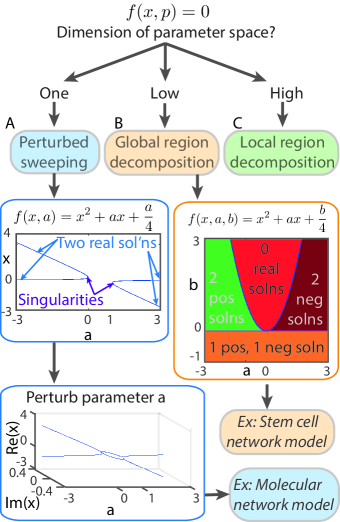
Figure 1. Flow chart of methods. (A) Linear perturbation. (B) Global method for decomposing $(a,b)$ parameter space into regions of number of real steady-states. (C) Local method for high dimensional parameter space analysis.

2.2. Quadratic Example

To illustrate the perturbed sweeping and global region decomposition approach, we consider two examples of a parameterized quadratic equation. The first has one parameter, namely $f(x,a)=x^{2}+ax+a/4$. The classical discriminant for quadratic polynomials yields $\Delta=a^{2}-a$ with discriminant locus $a=0,1$. In particular, $f=0$ has a singular real solution when $a=0$ or $a=1$, two distinct real solutions when $a<0$ or $a>1$, and two distinct nonreal solutions when $0<a<1$. To avoid tracking through the singularities, we use the perturbed sweeping method using $f(x,a+\epsilon i)=0$. In this case, for any fixed nonzero $\epsilon\in\mathbb{R}$ and $a\in\mathbb{R}$, $f(x,a+\epsilon i)=0$ always has 2 distinct solutions. By taking $\epsilon$ near zero, say $\epsilon=10^{-6}$, we sweep along the smooth curve parameterized by $a$ and observe the expected solution behavior as shown in Figure 1.

The second example has two parameters, namely $f(x,a,b)=x^{2}+ax+b/4$ and we aim to decompose the parameter space based on the number of real and positive solutions, which is typical in biological problems. The classical discriminant for quadratic polynomials yields $\Delta=a^{2}-b$ with the sign condition adding to this via the equation $f(0,a,b)=b/4=0$, i.e., $b=0$. Thus, the discriminant locus in this case consists of two irreducible curves which cut the parameter space $(a,b)\in\mathbb{R}^{2}$ into four regions where the number of real, positive, and negative solutions are constant on these regions as shown in Figure 1.

By using the projection $\pi(a,b)=a$, the perturbed sweeping method finds the critical point $a=0$ of the discriminant locus. For any $a<0$ or $a>0$, there are three regions in $b$, namely $b<0$, $0<b<a^{2}$, and $b>a^{2}$. For $a=0$, there are two regions in $b$, namely $b<0$ and $b>0$ which must extend away from $a=0$ by the implicit function theorem. Starting from one point in each of these regions, continuation is used to merge these $7$ regions into $4$ distinct regions of $\mathbb{R}^{2}$.

3. Results

We showcase our methods by applying them to two illustrative biological models: a detailed ODE model of the gene and protein signaling network that induces long-term memory proposed by Pettigrew et al. (28), and a network model of cell fate specification in a population of interacting stem cells. Since cellular decision making often depends on the number of accessible (stable) steady-states that a system exhibits, we seek to identify distinct regions of parameter space that can elicit different system behavior.

3.1. Molecular network model

A gene and protein network for long term memory was proposed by Pettigrew et al (28) and investigated using bifurcation and singularity analysis by Song et al. (29). The model developed is of the form of Eq. 1 where $\boldsymbol{f}$ consists of a total of $15$ polynomial and rational functions, $\boldsymbol{x}\in\mathbb{R}^{15}$ is the vector of 15 model variables, and $\boldsymbol{p}\in\mathbb{R}^{40}$ is a vector of 40 parameters.

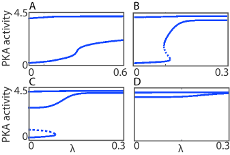
Figure 2. Perturbation sweeping method applied to molecular network of long term memory. $\lambda$ is the bifurcation parameter. Solid lines denote a stable steady-state, dashed lines denote an unstable steady-state. (A) Parameter $k_{34}=0.0022.$ (B) Parameter $k_{34}=0.015.$ (C) Parameter $k_{34}=0.03.$ (D) Parameter $k_{34}=0.1.$

The full system $\boldsymbol{f}$ is given in Appendix A for which the equations $\boldsymbol{f}(\boldsymbol{x},\boldsymbol{p})=0$ has $432$ isolated nonsingular solutions for general $\boldsymbol{p}$. The variable of interest required for long term facilitation is the steady-state of protein kinase A (PKA) in response to the extracellular stimulus parameter $\lambda$. Our aim is to demonstrate the sweeping perturbation method on a large model and reproduce the results in Fig. 5 of (29). We verify the two stable states and one unstable state, reproducing this figure. However we also find another solution not reported, demonstrating the power of this method (see top branch of Fig. 2). On inspection, this additional steady state is not on the same branch and is not biologically feasible so we can reject it as nonphysical. From this exhaustive first step of identifying and characterizing all the steady-states, one must exercise caution and systematically check each solution.

3.2. Cellular network model

Most multicellular organisms emerge from a small number of stem-like cells which become increasingly specialized as they proliferate until they transition to one of a finite number of differentiated states (30). We propose a caricature model of cell fate specification for a ring of cells, and investigate how cell-cell interactions, mediated by diffusive exchange of a key growth factor, may affect the number of (stable) configurations or patterns that the differentiated cells may adopt. The model serves as a good test case for discriminant locus methods since, by construction, there is an upper bound on the number of feasible steady states ($2^{N}$ solutions for a ring of $N$ cells) and some of these patterns are equivalent due to symmetries inherent in the governing equations.

In more detail, we consider a ring of interacting cells ($i=1,\dots,N$) and denote by $x_{i}(t)\geq 0$ the concentration within cell $i$ of a growth factor or protein (e.g., notch), whose value determines that cell’s differentiation status (31, 32, 33, 34, 35). The subcellular dynamics of $x_{i}$ are represented by a phenomenological function $q(x_{i})=-(x-\varepsilon)(a+x)(1-x)$ with $0<\varepsilon<a<1$, this function guaranteeing bistability of each cell in the absence of cell-cell communication. The bistability represents two distinct cell fates; e.g., high and low levels of notch may be associated with differentiation of intestinal epithelial cells into secretory and absorptive phenotypes differentiation (31, 32, 30). We assume further that cell $i$ communicates with its nearest neighbors (cells $i\pm 1$) via diffusive exchange of $x_{i}$ and denote by parameter $g\geq 0$ the coupling strength. Thus, our cell network model can be written

(2) $$\frac{dx_{i}}{dt}=q(x_{i})+g\cdot\sum_{j=i-1}^{i+1}(x_{j}-x_{i}),\text{ for all $i=1,\dots,N$.}$$

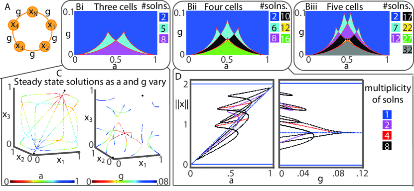
Figure 3. Global region decomposition applied to coupled cell network model. (A) Ring of cell network. Each cell $x_{i}$ has bistable dynamics at stable states at $0$ and $1$, and unstable state given by $a$. The cells are coupled to neighbor cells by a coupling strength parameter $g$. (B) Region decomposition with parameters $a,g$, similar to a classification diagram, with the number of real stable steady-stages denoted by different colors. The number of stable real steady-states is given for each network where $N=3,4,5$. (C) Steady-state values in state space for $N=3$ cell network are plotted as parameter $a$ is varied between $[\varepsilon,1]$ or $g$ is varied between 0 and 0.08. The two black dots are always a stable steady-states, the red is always an unstable steady-state, these steady-states are independent of parameter values $a$ and $g$. As the parameter value varies, the color changes according to the color bar. (D) Bifurcation diagram showing the 2-norm of $x$ as parameters are varied

We impose periodic boundary conditions so that $x_{N+1}\equiv x_{1}$ and $x_{0}\equiv x_{N}$, as shown in Fig. 3A. We analyze the model by applying the global decomposition method for $N=3,4,5$ cells, and construct classification diagrams in $(a,g)$ parameter space (Fig. 3B). We notice that intermediate values of $a$ generate the largest number of real stable steady-state; small and high values of $a$ yield fewer real stable steady-states. Interestingly, all cells synchronize for intermediate to strong values of the coupling parameter $g$ (two stable states in blue region in Fig 3B). We conclude that strong cell-cell communication reduces the number of stable steady state configurations that a population of cells can adopt and, thus, cell-cell communication could be used robustly to drive the cells to a small number of specific states. When coupling is weak ($0<g<0.1$), the interacting cells have more flexibility in terms of their final states, with the 5-cell network admitting up to 32 stable steady-states (Fig 3B(iii)). Weaker cell-cell communication allows more patterns to emerge and may be appropriate when it is less important that neighboring cells share the same phenotype. We find that the regions of $(a,g)$ parameter space that give rise to more than two (synchronized) steady states also increase in size as the number of cells increases.

In addition to decomposing parameter space into regions based on the multiplicity of steady solutions, the method also provides valuable information about how solution structure and stability change as system parameters vary. For example, in Fig. 3C for the $N=3$ cell network, we show how the values and stability of the steady-states for $(x_{1},x_{2},x_{3})$ change as $a$ varies with $g=0.025$ and as $g$ varies with $a=0.4$. In Fig. 3D, we plot bifurcation diagrams as $a$ and $g$ vary as before for the $N=4$ cell network; instead of presenting particular components $x_{i}$ ($i=1,2,3,4$), we plot the 2-norm ($\|\boldsymbol{x}\|=(x_{1}^{2}+x_{2}^{2}+x_{3}^{2}+x_{4}^{2})^{1/2}$) to capture the multiplicity of solutions. We note that for $N=3$ and $N=4$ there are always two stable and one unstable steady-states, independent of $(a,g)$ parameter values (as shown by the black and red points in Fig. 3C, and by the solid blue lines in Fig. 3D). We demonstrate the local region decomposition method to analyze a generalization of Eq. 2 to be cell specific by considering different cell-cell couplings (see Appendix B). Through this caricature stem-cell model, we have classified the steady-states, determined which are parameter-independent, explored changes in steady-state behavior as parameters are varied through the distinct regions of the parameter landscape.

4. Conclusion

We have presented a suite of new methods, based on computational algebraic geometry, for decomposing the parameter space associated with a dynamical system into distinct regions based on the multiplicity and stability of its steady-state solutions. The methods enable us to understand the parameter landscape of high-dimensional, ordinary differential models with large numbers of parameters. These methods have considerable potential: they could be used to analyze differential equation models associated with a wide range of real-world problems in biology, science and engineering which cannot be tackled with existing approaches.

We have demonstrated that groups of cells, especially cells that can have bistable internal dynamics, when coupled, increase the number of real stable steady-states. First we have considered all the cells to be homogeneous, and even with this simple model, we can gain new insight into how stem cells may transit into fully differentiated cells, with much richer dynamics, just by considering the interaction of the cells as a network. We considered different couplings between cells using a local region decomposition in the Appendix. We remark that it would be interesting to understand how a mutation in a single cell (for example, set $a$ very small) compares to real biological systems. In the future, it would be beneficial to consider different networks of cells (e.g., two growth factors, generalizations to 2D lattices) and the dynamical regimes these systems can admit.

By embracing and exploiting the complexity naturally present in biology, which often translates to nonlinearity in biological models, there is an incredible opportunity to develop and apply numerical algebraic geometric methods to study such models. With nonlinearity arising in all areas of science and engineering, the increasing complexity of various biological models provides a fertile testing ground for nonlinear approaches with a long-term goal of making numerical algebraic geometric methods as ubiquitous as methods in numerical linear algebra.

Appendix A The Song et al. model

For completeness, we reproduce below the system of 15 ordinary differential equations proposed by Song et al. (29). The parameters we vary are $\lambda=[5-HT]$ and $k_{34}$ = $k_{\mbox{ApSyn}}$. All other parameters are fixed to values given in (29).

(3) $$\frac{d[cAMP]}{dt} = 3.6\left(\frac{[5-HT]}{[5-HT]+14}\right)-([cAMP]-0.06)$$

(4) $$\frac{d[R]}{dt} = V_{\mbox{syn}}+k_{\mbox{fpka}}[RC][cAPM]^{2}-k_{\mbox{bpka}}[R][C]$$

$$-k_{\mbox{Ap-Uch}}[R]([\mbox{Ap-Uch}]_{\tau}-\mbox{Ap-Uch}_{\mbox{basal}})-k_{\mbox{dpka}}[R]$$

(5) $$\frac{d[C]}{dt} = V_{\mbox{syn}}+k_{\mbox{fpka}}[RC][cAPM]^{2}-k_{\mbox{bpka}}[R][C]$$

$$+k_{\mbox{Ap-Uch}}[RC]([\mbox{Ap-Uch}]_{\tau}-\mbox{Ap-Uch}_{\mbox{basal}})-k_{\mbox{dpka}}[C]$$

(6) $$\frac{d[RC]}{dt} = k_{\mbox{bpka}}[R][C]-k_{fpka}[RC][cAMP]^{2}$$

$$-k_{\mbox{Ap-Uch}}[RC]([\mbox{Ap-Uch}]_{\tau}-\mbox{Ap-Uch}_{\mbox{basal}})-k_{\mbox{dpka}}[RC]$$

(7) $$\frac{d[REG]}{dt} = k_{\mbox{translation}}[\mbox{mRNA}_{\mbox{REG}}]ERK_{\mbox{act}}$$

$$-v_{\mbox{dreg}}\left(\frac{[REG]}{[REG]+K_{\mbox{dreg}}}\right)-k_{\mbox{dsm}}[REG]$$

(8) $$\frac{d[pREG]}{dt} = v_{\mbox{rphos}}ERK_{\mbox{act}}\left(\frac{[REG]-[pREG]}{[REG]-[pREG]+K_{\mbox{rphos}}}\right)-v_{\mbox{dreg}}\left(\frac{[pREG]}{[REG]+K_{\mbox{dreg}}}\right)$$

$$-k_{\mbox{dsm}}[\mbox{pREG}]$$

(9) $$\frac{d[\mbox{mRNA}_{\mbox{REG}}]}{dt} = v_{\mbox{mREG}}-v_{\mbox{dmreg}}[5-HT]\left(\frac{[\mbox{mRNA}_{\mbox{REG}}]}{[\mbox{mRNA}_{\mbox{REG}}]+K_{\mbox{dmreg}}}\right)-k_{\mbox{dmreg}}[\mbox{mRNA}_{\mbox{REG}}]$$

(10) $$\frac{d[\mbox{Raf}]}{dt} = -k_{f,\mbox{Raf}}[5-HT][Raf]+k_{b,\mbox{Raf}}[\mbox{Raf}^{p}]$$

(11) $$\frac{d[\mbox{MAPKK}]}{dt} = -k_{f,\mbox{MAPKK}}[\mbox{Raf}^{p}]\left(\frac{[\mbox{MAPKK}]}{[\mbox{MAPKK}]+K_{\mbox{MK}}}\right)+k_{b,\mbox{MAPKK}}\left(\frac{[\mbox{MAPKK}^{p}]}{[\mbox{MAPKK}^{p}]+K_{\mbox{MK}}}\right)$$

(12) $$\frac{d[MAPKK]^{pp}}{dt} = k_{f,\mbox{MAPKK}}[\mbox{Raf}^{p}]\left(\frac{[\mbox{MAPKK}^{p}]}{[\mbox{MAPKK}^{p}]+K_{\mbox{MK}}}\right)-k_{b,\mbox{MAPKK}}\left(\frac{[\mbox{MAPKK}^{pp}]}{[\mbox{MAPKK}^{pp}]+K_{\mbox{MK}}}\right)$$

(13) $$\frac{d[\mbox{ERK}]}{dt} = -k_{f,\mbox{ERK}}[\mbox{MAPKK}^{pp}]\left(\frac{[\mbox{ERK}]}{[\mbox{ERK}]+K_{\mbox{MK}}}\right)+k_{b,\mbox{ERK}}\left(\frac{[\mbox{ERK}^{p}]}{[\mbox{ERK}^{p}]+K_{\mbox{MK}}}\right)$$

(14) $$\frac{d[\mbox{ERK}^{pp}]}{dt} = k_{f,\mbox{ERK}}[\mbox{MAPKK}^{pp}]\left(\frac{[\mbox{ERK}^{p}]}{[\mbox{ERK}^{p}]+K_{\mbox{MK}}}\right)-k_{b,\mbox{ERK}}\left(\frac{[\mbox{ERK}^{pp}]}{[\mbox{ERK}^{pp}]+K_{\mbox{MK}}}\right)$$

(15) $$\frac{dP_{\mbox{pka}}}{dt} = k_{\mbox{phos1}}\mbox{PKA}_{\mbox{act}}(1-P_{\mbox{pka}})-k_{\mbox{dephos1}}\mbox{PPhos}P_{\mbox{pka}}$$

(16) $$\frac{dP_{\mbox{erk}}}{dt} = k_{\mbox{phos2}}\mbox{ERK}_{\mbox{act}}(1-P_{\mbox{erk}})-k_{\mbox{dephos2}}\mbox{PPhos}P_{\mbox{erk}}$$

(17) $$\frac{d[\mbox{AP-Uch}]}{dt} = k_{\mbox{ApSyn}}\left(\frac{P^{2}_{\mbox{pka}}}{P^{2}_{\mbox{pka}}+K^{2}_{\mbox{pka}}}\right)\left(\frac{P^{2}_{\mbox{erk}}}{P^{2}_{\mbox{erk}}+K^{2}_{\mbox{erk}}}\right)+k_{\mbox{ApSynBasal}}-k_{\mbox{deg}}[\mbox{Ap-Uch}]$$

where

$$PKA_{\mbox{act}} = [C],$$

$$\left[\mbox{Raf}^{p}\right] = [\mbox{Raf}_{\mbox{tot}}]-[\mbox{Raf}],$$

$$k_{\mbox{bpka}} = \left(\frac{k_{\mbox{baspka}}}{1+[pREG]/K_{\mbox{reg}}}\right),$$

$$\left[\mbox{ERK}^{p}\right] = [\mbox{ERK}_{\mbox{tot}}]-[\mbox{ERK}]-[\mbox{ERK}^{pp}],$$

$$\mbox{ERK}_{\mbox{act}} = [\mbox{ERK}^{pp}]+\mbox{ERK}_{\mbox{basal}},$$

$$\left[\mbox{MAPKK}^{p}\right] = [\mbox{MAPKK}_{\mbox{tot}}]-[\mbox{MAPKK}]-[\mbox{MAPKK}^{pp}].$$

Following (29), we fix the model parameters at the following values:

$$V_{\mbox{syn}} = 0.002\mbox{min}^{-1},k_{\mbox{fpka}}=105.0\mbox{min}^{-1},$$

$$k_{\mbox{Ap-Uch}} = 0.007\mbox{min}^{-1},\mbox{Ap-Uch}_{\mbox{basal}}=0.10,$$

$$k_{\mbox{dpka}} = 0.00048\mbox{min}^{-1},\tau=250\mbox{min},$$

$$k_{\mbox{baspka}} = 12\mbox{min}^{-1},k_{\mbox{reg}}=0.00064,$$

$$k_{\mbox{translation}} = 4\mbox{min}^{-1},v_{\mbox{rphos}}=1\mbox{min}^{-1},K_{\mbox{rphos}}=1.5,$$

$$v_{\mbox{dreg}} = 0.16\mbox{min}^{-1},K_{\mbox{dreg}}=0.0015,$$

$$k_{\mbox{dsm}} = 0.02\mbox{min}^{-1},v_{\mbox{mREG}}=2^{-5}\mbox{min}^{-1},$$

$$v_{\mbox{dmreg}} = 0.00225\mbox{min}^{-1},K_{\mbox{dmreg}}=0.01,$$

$$k_{\mbox{dmreg}} = 3\times 10^{-5}\mbox{min}^{-1},k_{f,\mbox{Raf}}=0.00345\mbox{min}^{-1},$$

$$k_{f,\mbox{MAPKK}} = 0.7\mbox{min}^{-1},k_{f,\mbox{ERK}}=0.44\mbox{min}^{-1},$$

$$k_{b,\mbox{Raf}} = 0.001\mbox{min}^{-1},k_{b,\mbox{MAPKK}}=0.12\mbox{min}^{-1},$$

$$k_{b,\mbox{ERK}} = 0.12\mbox{min}^{-1},[\mbox{Raf}_{\mbox{tot}}]=0.5,$$

$$\mbox{MAPKK}_{\mbox{tot}} = 0.5,[ERK_{\mbox{tot}}]=0.5$$

$$K_{\mbox{MK}} = 0.08,\mbox{ERK}_{\mbox{basal}}=0.015,$$

$$k_{\mbox{phos1}} = 0.01\mbox{min}^{-1},k_{\mbox{dephos1}}=1.5\mbox{min}^{-1},$$

PPhos $$= 0.1,k_{\mbox{phos2}}=0.005\mbox{min}^{-1},$$

$$k_{\mbox{ApSyn}} = 0.02\mbox{min}^{-1},k_{\mbox{ApSynBasal}}=0.0009\mbox{min}^{-1},$$

$$K_{\mbox{pka}} = 0.2,K_{\mbox{erk}}=0.004,$$

$$k_{\mbox{deg}} = 0.01\mbox{min}^{-1}$$

We remark that the discriminant method can handle rational functions. For this example, the denominators do not vanish near the regions of interest so they do not have any impact on the behavior of the solutions. If the denominator also vanished when finding a solution to the system of equations from the numerators, then the parameter values for which this occurs would be added into the discriminant locus.

Appendix B Cell network model

The model in Eq. 2 used uniform coupling $g$ for all nearest neighbors. Using (36), as a set, the classical discriminant locus for this model with $N=4$ has degree $72$. That is, there is a degree $72$ polynomial $\Delta(a,g)$ such that the classical discriminant locus is defined by $\Delta=0$. With $a=0.4$ as in Fig 3D, the univariate polynomial equation $\Delta(0.4,g)=0$ has $45$ complex solutions, $25$ of which are real with $15$ positive with only $4$ corresponding to a change in the number of stable steady-state solutions yielding the regions (intervals) for $g$ approximately:

$${\small\begin{array}[]{r|ccccc}\mbox{regions}&[0,0.0197)&(0.0197,0.0206)&(0.0206,0.0411)&(0.0411,0.0533)&(0.0533,\infty)\\ \hline\cr\mbox{\# stable steady-state solns}&16&12&10&6&2\end{array}}$$

We now consider a generalization of this model which uses coupling strengths $g_{i,i+1}=g_{i+1,i}\geq 0$ between cell $i$ and $i+1$ with cyclic ordering ($N+1\equiv 1$), namely

(18) $$\frac{dx_{i}}{dt}=q(x_{i})+\sum_{j=i-1}^{i+1}g_{i,j}\cdot(x_{j}-x_{i}),\text{ for all $i=1,\dots,N$.}$$

With $N=4$, as a set, the classical discriminant locus for this generalized model has degree $486$. We consider the case with $a=0.4$ and $g_{4,1}=g_{1,4}=0$ leaving three free parameters $g_{1,2}$, $g_{2,3}$, and $g_{3,4}$.

The perturbed sweeping approach along the ray defined by $g_{i,i+1}=i\cdot t$ for $i=1,2,3$ and $t\geq 0$ decomposes the space $t\geq 0$ into $15$ regions, approximately

$$\begin{array}[]{c|c}\mbox{regions}&\mbox{\# stable steady-state solns}\\ \hline\cr[0,0.0079)&16\\ (0.0079,0.0080)&15\\ (0.0080,0.0132)&14\\ (0.0132,0.0136)&13\\ (0.0136,0.0137)&12\\ (0.0137,0.0142)&11\\ (0.0142,0.0153)&10\\ (0.0153,0.0161)&9\\ (0.0161,0.0171)&8\\ (0.0171,0.0237)&7\\ (0.0237,0.0352&6\\ (0.0352,0.0360)&5\\ (0.0360,0.0407)&4\\ (0.0407,0.1264)&3\\ (0.1264,\infty)&2\end{array}$$

As a comparison, the classical discriminant with respect to $t\in\mathbb{C}$ consists of $312$ distinct points of which $84$ are real with $42$ positive with $14$ corresponding to a change in the number stable steady-state solutions. Figure 4 plots the region with $16$ stable steady-state solutions along various rays emanating from the origin.

Figure 4. Plot of the regions with $16$ stable steady-state solutions along various rays emanating from $g_{1,2}=g_{2,3}=g_{3,4}=0$.

References

- (1) Collins GE (1975) in Automata theory and formal languages (Second GI Conf., Kaiserslautern, 1975) (Springer, Berlin), pp 134–183. Lecture Notes in Comput. Sci., Vol. 33.
- (2) Lazard D, Rouillier F (2007) Solving parametric polynomial systems. Journal of Symbolic Computation 42:636 – 667.
- (3) Xia B (2007) Discoverer: a tool for solving semi-algebraic systems. ACM Communications in Computer Algebra 41:102–103.
- (4) Brown CW (2003) Qepcad b: a program for computing with semi-algebraic sets using cads. ACM SIGSAM Bulletin 37:97–108.
- (5) Cox DA, Little J, O’Shea D (2005) Using algebraic geometry, Graduate Texts in Mathematics (Springer, New York) Vol. 185, Second edition.
- (6) Gel′fand IM, Kapranov MM, Zelevinsky AV (1994) Discriminants, resultants, and multidimensional determinants, Mathematics: Theory & Applications (Birkhäuser Boston, Inc., Boston, MA).
- (7) Sturmfels B (2002) Solving systems of polynomial equations, CBMS Regional Conference Series in Mathematics (Published for the Conference Board of the Mathematical Sciences, Washington, DC; by the American Mathematical Society, Providence, RI) Vol. 97.
- (8) Doedel EJ (1981) Auto: A program for the automatic bifurcation analysis of autonomous systems. Congr. Numer 30:265–284.
- (9) Dhooge A, Govaerts W, Kuznetsov YA (2003) Matcont: a matlab package for numerical bifurcation analysis of odes. ACM Transactions on Mathematical Software (TOMS) 29:141–164.
- (10) Bates DJ, Hauenstein JD, Sommese AJ, Wampler CW (2013) Numerically solving polynomial systems with Bertini (SIAM) Vol. 25.
- (11) Sommese AJ, Wampler, II CW (2005) The numerical solution of systems of polynomials (World Scientific Publishing Co. Pte. Ltd., Hackensack, NJ) Arising in engineering and science.
- (12) Wampler C, Sommese A, Morgan A (1990) Numerical continuation methods for solving polynomial systems arising in kinematics. Journal of mechanical design 112:59–68.
- (13) Bates DJ, Hauenstein JD, Sommese AJ, Wampler II CW (2008) in Software for algebraic geometry (Springer), pp 1–14.
- (14) Chen T, Lee TL, Li TY (2014) in Mathematical software—ICMS 2014, Lecture Notes in Comput. Sci. (Springer, Heidelberg) Vol. 8592, pp 183–190.
- (15) Verschelde J (1999) Algorithm 795: Phcpack: A general-purpose solver for polynomial systems by homotopy continuation. ACM Transactions on Mathematical Software (TOMS) 25:251–276.
- (16) Bates DJ, Brake DA, Niemerg ME (2015) Paramotopy: Parameter homotopies in parallel. (Available at paramotopy.com).
- (17) Hao W, Hauenstein JD, Hu B, Sommese AJ (2011) A three-dimensional steady-state tumor system. Appl. Math. Comput. 218:2661–2669.
- (18) Piret K, Verschelde J (2010) Sweeping algebraic curves for singular solutions. J. Comput. Appl. Math. 234:1228–1237.
- (19) Lu Y, Bates DJ, Sommese AJ, Wampler CW (2007) in Algebra, geometry and their interactions, Contemp. Math. (Amer. Math. Soc., Providence, RI) Vol. 448, pp 183–205.
- (20) Bates DJ, Brake DA, Hauenstein JD, Sommese AJ, Wampler CW (2014) in Mathematical software—ICMS 2014, Lecture Notes in Comput. Sci. (Springer, Heidelberg) Vol. 8592, pp 246–252.
- (21) Besana GM, Di Rocco S, Hauenstein JD, Sommese AJ, Wampler CW (2013) Cell decomposition of almost smooth real algebraic surfaces. Numer. Algorithms 63:645–678.
- (22) Niu W, Wang D (2008) Algebraic approaches to stability analysis of biological systems. Mathematics in Computer Science 1:507–539.
- (23) Hanan W, Mehta D, Moroz G, Pouryahya S (2010) Stability and bifurcation analysis of coupled fitzhugh-nagumo oscillators. ”Extended abstract” published in the Joint Conference of ASCM2009 and MACIS2009, Japan, 2009. arXiv:1001.5420.
- (24) Hernandez-Vargas EA, Mehta D, Middleton RH (2011) Towards modeling hiv long term behavior. Proceedings of 18th IFAC World Congress, Milan, 2011. arXiv:1105.2823.
- (25) Gross E, Harrington HA, Rosen Z, Sturmfels B (2016) Algebraic systems biology: A case study for the wnt pathway. Bulletin of Mathematical Biology 78:21–51.
- (26) Golubitsky M, Schaeffer DG (1985) Singularities and groups in bifurcation theory. Vol. I, Applied Mathematical Sciences (Springer-Verlag, New York) Vol. 51, pp xvii+463.
- (27) Griffin ZA, Hauenstein JD (2015) Real solutions to systems of polynomial equations and parameter continuation. Adv. Geom. 15:173–187.
- (28) Pettigrew DB, Smolen P, Baxter DA, Byrne JH (2005) Dynamic properties of regulatory motifs associated with induction of three temporal domains of memory in aplysia. Journal of computational neuroscience 18:163–181.
- (29) Song H, Smolen P, Av-Ron E, Baxter DA, Byrne JH (2006) Bifurcation and singularity analysis of a molecular network for the induction of long-term memory. Biophysical journal 90:2309–2325.
- (30) Clevers H (2015) STEM CELLS. What is an adult stem cell? Science 350:1319–1320.
- (31) Fre S, et al. (2005) Notch signals control the fate of immature progenitor cells in the intestine. Nature 435:964–968.
- (32) Sprinzak D, et al. (2010) Cis-interactions between Notch and Delta generate mutually exclusive signalling states. Nature 465:86–90.
- (33) Yeung TM, Chia LA, Kosinski CM, Kuo CJ (2011) Regulation of self-renewal and differentiation by the intestinal stem cell niche. Cellular and molecular life sciences : CMLS 68:2513–2523.
- (34) Visvader JE, Clevers H (2016) Tissue-specific designs of stem cell hierarchies. Nat Cell Biol 18:349–355.
- (35) Grün D, et al. (2015) Single-cell messenger RNA sequencing reveals rare intestinal cell types. Nature 525:251–255.
- (36) Hauenstein JD, Sommese AJ (2010) Witness sets of projections. Appl. Math. Comput. 217:3349–3354.