Modeling the near-wake of a vertical-axis cross-flow turbine with 2-D and 3-D RANS
Abstract
The near-wake of a vertical-axis cross-flow turbine (CFT) was modeled numerically via blade-resolved – SST and Spalart–Allmaras RANS models in two and three dimensions. Results for each case are compared with experimental measurements of the turbine shaft power, overall drag, mean velocity, turbulence kinetic energy, and momentum transport terms in the near-wake at one diameter downstream. It was shown that 2-D simulations overpredict turbine loading and do not resolve mean vertical momentum transport, which plays an important role in the near-wake’s momentum balance. The 3-D simulations fared better at predicting performance, with the Spalart–Allmaras model predictions being closest to the experiments. The SST model more accurately predicted the turbulence kinetic energy while the Spalart–Allmaras model more closely matched the momentum transport terms in the near-wake. These results show the potential of blade-resolved RANS as a design tool and a way to “extrapolate” experimental flow field measurements.
I Introduction
In the pursuit of a fully sustainable energy profile, cross-flow (often vertical-axis) turbines (CFTs) can still play a role. Despite extensive research and development in the 1970s through the early 1990s by groups like Sandia National Labs in the US Sutherland, Berg, and Ashwill (2012) and the National Research Council in Canada Paraschivoiu (2002), the vertical-axis cross-flow Darrieus turbines were all but abandoned for large scale commercial terrestrial wind power. Today, however, with the development of marine hydrokinetic (MHK) energy devices, CFTs are at the forefront, with the first grid-connected commercial device being a horizontal-axis CFT manufactured and installed by ORPC in Cobscook Bay, Maine Ocean Renewable Power Company (2012). CFTs are also being examined for small-scale onshore wind in urban areas Lott (2015), offshore floating wind farms Paulsen et al. (2011); Sandia National Laboratories (2012), and onshore wind farms where power output per unit land area is of interest Dabiri (2011).
Despite the development of many simple engineering models based on blade element momentum or vortex methods, it remains difficult to predict the performance of cross-flow turbines for all cases—namely when solidity, or blade chord-to-radius ratio is high—a common characteristic of smaller rotors, and those designed for marine hydrokinetic (MHK) applications. With computing power becoming evermore available and affordable, CFD based on the Reynolds-averaged Navier–Stokes (RANS) equations has become an attractive method for predicting the performance of cross-flow turbines. Since a direct numerical simulation (DNS) of all scales at realistic Reynolds numbers is not currently feasible, turbulence be modeled. However, with an appropriate turbulence model, blade-resolved RANS presents a more physically realistic first principles based approach versus simpler models based on momentum theory or potential flow. However, CFD can be computationally expensive when done in three dimensions, which may be necessary in some cases.
There are many examples in the literature of 2-D cross-flow turbine simulations with widely varying results. Balduzzi et al. Balduzzi et al. (2016) provides a summary of recent efforts and an attempt to standardize a methodology for using Reynolds-averaged Navier–Stokes (RANS) to correctly predict performance of a 2-D CFT. Howell et al. Howell et al. (2010), performed both 2-D and 3-D simulations of a high solidity cross-flow turbine using a – renormalization group (RNG) turbulence model. The results from the 2-D simulations over-predicted power coefficient, while the 3-D case matched well with wind tunnel measurements near the tip speed ratio of maximum power. In general, 3-D simulations are less common, but have begun to appear more frequently recently—a testament to the progress towards higher computing power.
An overview of 3-D blade-resolved cross-flow turbine simulations reported in the literature is presented in Table 1. The – SST RANS turbulence model is shown to be a popular choice due to its success in predicting flows with adverse pressure gradients and separation Menter, Kuntz, and Langtry (2003). Higher fidelity methods that resolve the large scales of turbulence, such as large eddy and detached eddy simulation have also been used. Note that for all the studies listed, model validation was performed for either performance or wake predictions—not both—and in some case omitted entirely.
| Author | Turbulence modeling | Perf. val. | Wake val. |
|---|---|---|---|
| Alaimo et al. Alaimo et al. (2015) | – RANS | N/A | N/A |
| Marsh et al. Marsh et al. (2015) | SST RANS | Reference Rawlings (2008) | N/A |
| Orlandi et al. Orlandi et al. (2015) | SST RANS | References Akins (1989); Mertens, van Kuik, and van Bussel (2003) | N/A |
| Lam & Peng Lam and Peng (2016) | SST RANS & IDDES | N/A | Reference Tescione et al. (2014) |
| Nini et al. Nini et al. (2014) | Spalart–Allmaras RANS | N/A | Reference Battisti et al. (2011) |
| Boudreau & Dumas Boudreau and Dumas (2015) | Spalart–Allmaras DDES | N/A | N/A |
| Li et al. Li et al. (2013) | SST RANS & Smagorinsky–Lilly LES | Reference McLaren (2011) | N/A |
| Howell et al. Howell et al. (2010) | – RNG RANS | Reference Howell et al. (2010) | N/A |
Modeling the boundary layer flows on cross-flow turbine blades is essential to predicting the blade loading. This flow condition presents a challenge due to the dynamically changing inflow velocity and angle of attack—which often exceeds static stall values and causes dynamic stall. Furthermore, the ability to predict the occurrence and interdependence of boundary layer transition to turbulence and separation can have dramatic influence on the blade loading and therefore the predicted turbine power output. These challenges present significant obstacles to the prospect of using CFD to replace wind tunnel or tank testing of physical models.
To date, little computational work has been done to attempt to design arrays of CFTs, despite their prospects for closer spacing compared with axial-flow turbines (AFTs). For example, Araya et al. Araya et al. (2014) modeled the flow through a VAT array using “leaky Rankine body” potential flow singularities, which was able to rank relative—though not absolute—performance of array configurations. Goude and Agren Goude and Agren (2010) used a 2-D vortex method to simulate a farm of cross-flow turbines, though this was not validated with experiments. Durrani et al. Durrani et al. (2011) used 2-D CFD to model a group of cross-flow turbines, observing higher power output for a staggered configuration, but also did not compare with experimental results. Giorgetti et al. Giorgetti, Pellegrini, and Zanforlin (2015) took a similar approach for 2-D array analysis using turbine pairs inspired by Dabiri Dabiri (2011), but again experimental validation was not performed. Li and Calisal Li and Calisal (2010) used a 3-D vortex line method to show mutually improved power output from two adjacent turbines, though the simulations over-predicted the effects by approximately 5% compared with experiments. Antheaume et al. Antheaume, Maître, and Achard (2008) used a blade element approach coupled with a 3-D RANS solver to also show how close spacing can improve power output of CFTs.
In this study we set out to model the performance and near-wake of the high solidity University of New Hampshire Reference Vertical-Axis Turbine (UNH-RVAT) using the Reynolds-averaged Navier–Stokes equations using the open-source finite volume CFD package OpenFOAM, version 2.3.x. Though studies in the literature generally focus on predicting the turbine loading and the local blade boundary layer, we seek to model both this and the larger scale flow produced by the rotor, i.e., the near-wake, which is of interest for this particular turbine since it has been shown experimentally that the near-wake’s momentum and energy transport processes are dominated by vertical advection Bachant and Wosnik (2015). It logically follows that a 2-D simulation, which omits the vertical dimension, would not correctly predict wake recovery and turbine–turbine interaction. However, it is of interest to determine how wrong a 2-D model may be, since the lower computational cost of 2-D simulations is attractive.
We seek to validate 2-D and 3-D blade-resolved RANS models against the UNH-RVAT mechanical power and near-wake measurements. If the blade loading and velocity in the near-wake match well enough, the flow field can potentially be inspected in greater detail, i.e., we may be able to make observations of quantities not measured experimentally, e.g., pressure, and gain greater insight into where the dominant flow structures originate. This will ultimately help develop and evaluate low-order wake generator models for use in turbine array modeling. In summary, the questions we hope to answer here are:
-
1.
Can 2-D RANS be used for individual turbine and/or array design?
-
2.
How accurately can 3-D RANS predict performance?
-
3.
Do the flow fields predicted by 3-D RANS match the experimental wake measurements well enough to provide insight for developing new low-order wake generators to represent CFTs?
-
4.
Does 3-D RANS realize the correct proportions of wake recovery mechanisms, i.e., are the 3-D blade-resolved results a good reference case or “target” for those a low-order model should produce?
II Numerical setup
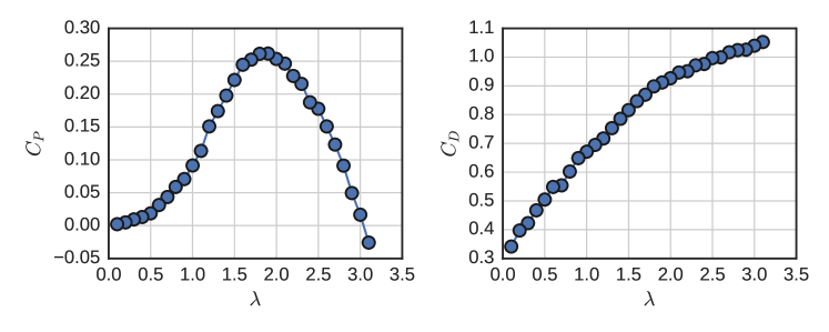
In this study the UNH-RVAT baseline tow tank experiment was simulated using a mean rotor tip speed ratio , which corresponds to the maximum measured power coefficient; cf. Figure 1. The tow speed or free stream velocity m/s gives a turbine diameter Reynolds number , which corresponds to the -independent state for both performance and near-wake characteristics, as determined from previous experimental measurements Bachant and Wosnik (2014, 2016a).
The turbines CAD geometry was prepared or “cleaned” for CFD by removing details determined to be unnecessary, e.g., screw heads and axial shaft grooves, which would complicate the meshing process and contribute very little to the overall loading or flow modulation. A drawing of the physically and numerically modeled geometries is presented in Figure 2.

To close the RANS equations, two different turbulence models were used: Menter’s – SST Menter (1994) and the Spalart–Allmaras (SA) one equation model Spalart and Allmaras (1992). Both closures use the eddy-viscosity approach—the SA employing a single additional scalar transport equation for an eddy-viscosity-like quantity and the SST solving equations for the turbulence kinetic energy and specific dissipation . The SST model was chosen due to its prominence in the literature for simulating separating flows, which we assumed to be present in the current problem in the form of dynamic stall. The SA model was shown by Ferreira et al. Ferreira et al. (2007) to match experimental particle image velocimetry (PIV) results for a CFT in dynamic stall, though this was a somewhat low Reynolds number case (). Further justification for using the SA model for this case comes from Crivellini and D’Alessandro Crivellini and D’Alessandro (2014), where they successfully modeled the laminar separation bubble and subsequent boundary layer transition to turbulence at Reynolds numbers similar to those investigated here.
II.1 Computational mesh
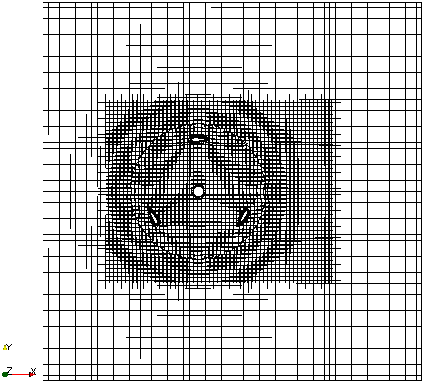
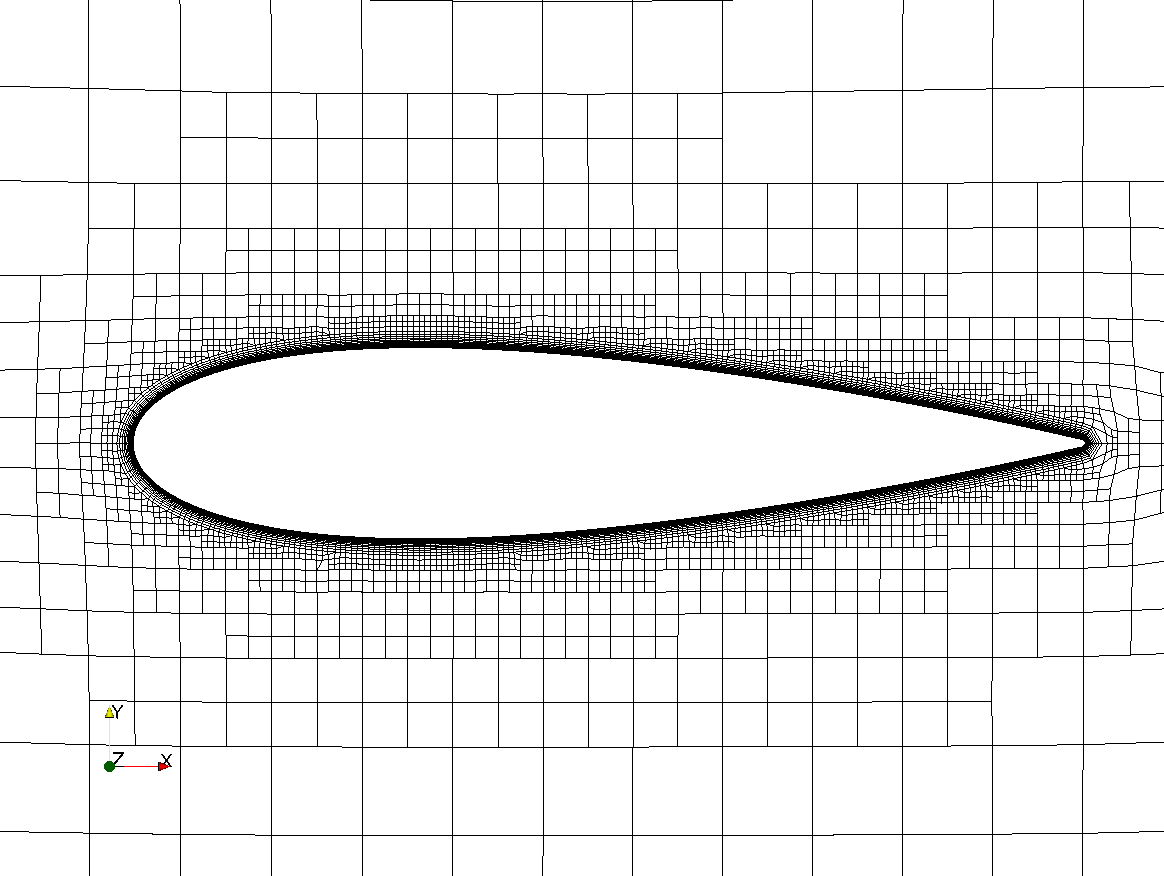
The computational domain was a rectangular volume 3.66 m long, 3.66 m wide, and 2.44 m tall (for 3-D), with the turbine located 1.52 m from the inlet, and centered vertically with a vertical axis, designed to match the tow tank dimensions for comparison with previous experiments. The rotor geometry was located at the center of a cylindrical sliding mesh interface, which rotated at a mean tip speed ratio with a sinusoidal oscillation at the blade passage frequency—with and amplitude of 0.19 and the first peak at 1.4 radians—to mimic the slight deviation from the mean tip speed ratio observed in the experiments. The 2-D mesh overview is shown in Figure 3 and the blade mesh detail is shown in Figure 4.
Meshes were generated using OpenFOAM’s blockMesh and snappyHexMesh utilities. Mesh topology consists of a background hexahedral mesh, which is refined in all three directions by a factor of 2 in a rectangular region containing the turbine and near-wake (0.9 m upstream, 1.3 m downstream, m cross-stream, and m vertically). Cells adjacent to the turbine shaft and struts are refined by a factor of 4, while cells adjacent to the blades are refined by a factor of 6. To capture the boundary layer, 20 layers were added next to the blades with an expansion ratio of 1.2. Overall mesh refinement is controlled by a single parameter—the number of cells in the streamwise direction, .
II.2 Solver
Simulations were run using OpenFOAM’s pimpleDyMFoam solver, which uses a hybrid PISO-SIMPLE algorithm for pressure-velocity coupling and is compatible with dynamic meshes. An Euler scheme was used to advance the simulation forward in time. The case files required to replicate the simulations are available from Bachant (2016a, b, c, d).
II.3 Initial and boundary conditions
Initial and boundary conditions were set to match those of the tow tank as well as possible. The velocity at the inlet, bottom, and side walls was fixed to 1 m/s to match the tow tank case, while the top boundary condition was a slip velocity condition. Pressure was held fixed at the outlet while a zero-gradient boundary condition was applied at the inlet (a typical velocity-inlet/pressure-outlet case). Note that in 2-D the top and bottom boundary conditions are “empty,” which is an OpenFOAM convention to indicate two-dimensionality.
Since the mesh was only refined next to the blade surfaces in order to resolve the boundary layer profile, no wall functions were used. However, wall functions were used for the other turbine surfaces, i.e., struts, hub, and shaft, and for the tank sidewalls, bottom, and top.
III Model verification
Both the – SST and Spalart–Allmaras RANS model cases were verified for convergence of the turbine mean power coefficient with respect to grid spacing and time step using 2-D domains. The grid topology was fixed, but the number of cells per domain length was scaled proportionally, maintaining the same background mesh cell aspect ratio. Results for this parameter sweep are shown in Figure 5, from which the final number of streamwise grid points was chosen, which resulted in a nondimensional wall distance , where is the friction velocity, defined as , where is the wall shear stress. This mesh resolution gave a total cell count of approximately for the 2-D cases and 16 million for the 3-D case. Sensitivity to domain length was assessed as well, showing a 2% increase in mean power coefficient for the 2-D SST case with the domain extended an additional two rotor diameters downstream.
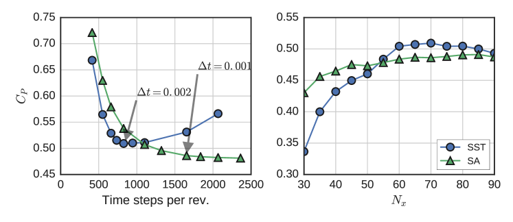
Time step dependence was evaluated using the 2-D grid, the results from which are shown in Figure 5. It was seen that the Spalart–Allmaras model converged well with decreasing time step, leading to a final time step of 0.001 s. The results from the SST model show a local minimum at s, with some divergence for smaller time steps. The local minimum was chosen as the final time step to run the simulations. Note that the SST model’s convergence behavior may be due to its specific implementation in OpenFOAM, and not indicative of the nature of the model equations. Verification studies for CFTs with this level of detail in the literature are not common, though the final time step is comparable to others Balduzzi et al. (2016).
IV Results
Turbine operation in all cases was simulated for 10 seconds, or approximately six rotor revolutions. Computations for the 3-D cases were run on 192 processes (24 nodes 8 cores each on Sandia National Labs’ Red Mesa high performance computing cluster) and took on the order of 1,000 CPU hours per second of simulated time. The 2-D simulations were run on a single processor and took on the order of one CPU hour per second.
Performance statistics were computed after the first revolution onward and flow statistics were calculated over the time interval spanning – seconds, or approximately three rotor revolutions, from time series downsampled to 50 Hz. It is assumed that the downsampling frequency is high enough above the blade passage frequency such that differences from the variance (for computing turbulence statistics) in the original velocity will be negligible.
IV.1 Performance prediction
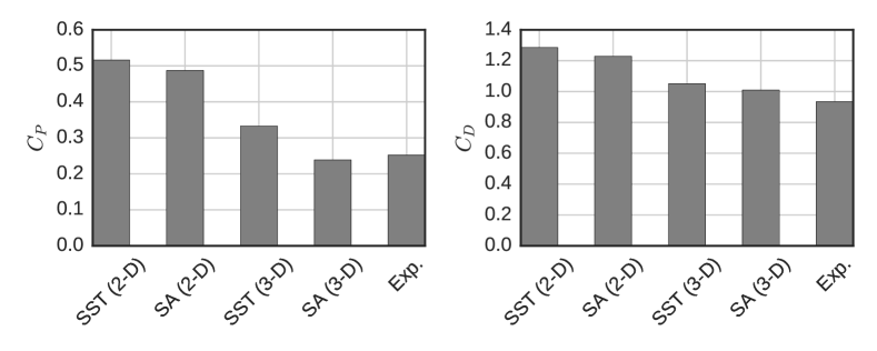
Predictions for both the mean rotor power and drag coefficients are shown in Figure 6. In general, the 2-D CFD cases both significantly overpredict turbine loading and therefore mechanical power output, which is due to their increased blockage ratio, unresolved blade end effects, and lack of blade support struts.
The 3-D simulations matched the experimental measurements more closely. The Spalart–Allmaras model’s mean power coefficient was 0.24 while the SST’s was 0.33, which represent a 6% under- and 30% overprediction, respectively, compared with the experiments. Some of the apparent overprediction of rotor drag coefficient could also be an effect of the experimental procedure, where the “tare drag” from the turbine mounting structure was measured without a turbine installed, then subtracted in post-processing. With the turbine installed, flow past the mounting frame will be higher due to blockage, meaning the tare drag would be underestimated, and the CFD results for should be slightly higher than the experimental measurements.
IV.2 Wake characteristics
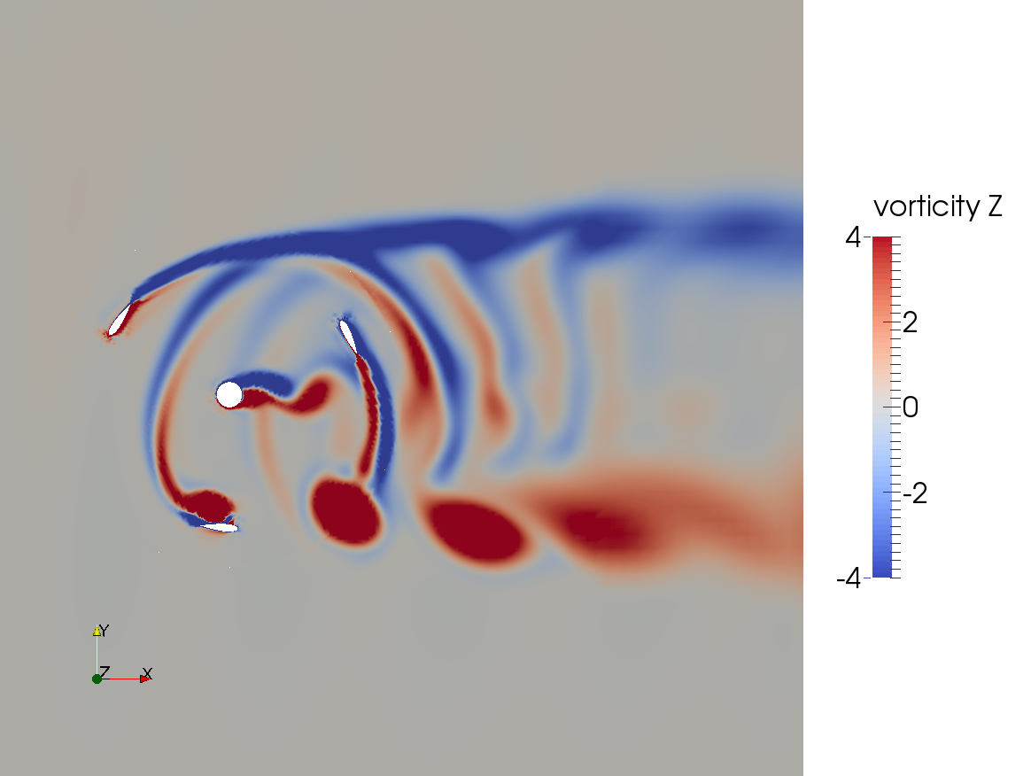
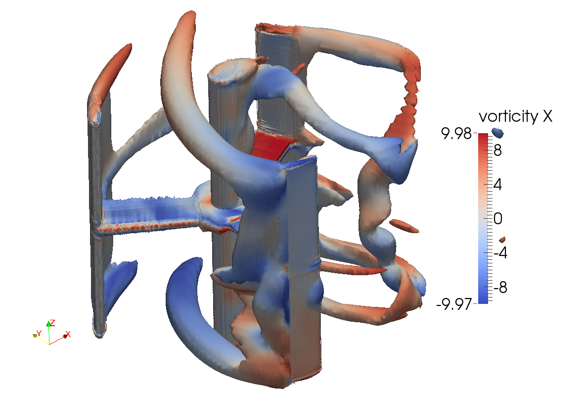
Visualizations of the complex vorticity field generated by the turbine are presented for the 2-D and 3-D Spalart–Allmaras cases in Figure 7 and Figure 8, respectively. It can be seen how the upstream blade—as it turns back into the streamwise direction—is shedding a large amount of spanwise vorticity due to the separated flow. In the 3-D case, strong tip vortices are also present, which trace the “contracting” wake flow on the side of the turbine associated with the induced vertical velocity field. The 3-D dynamic stall vortex also shows asymmetry about the – mid-rotor plane; once again highlighting the importance of three-dimensional effects on wake dynamics.
Mean velocity profiles at one turbine diameter downstream are shown in Figure 9. The 2-D results suffer from a blockage mismatch, i.e., keeping the proximity of the walls constant increases the blockage ratio. The 3-D results, however, show good agreement with the experiments.
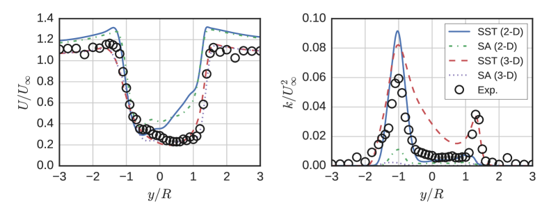
Turbulence kinetic energy profiles are also shown in Figure 9. The turbulence kinetic energy for the unsteady RANS models was calculated as
| (1) |
where (the resolved velocity fluctuations) and is the kinetic energy calculated by the turbulence model, which is zero for the SA model.
Both Spalart–Allmaras cases did a poor job predicting the turbulence kinetic energy in the flow, since it must be resolved as variance in the velocity field. The 2-D SST model did a good job predicting the peak in at , though is missing the smaller peak at . This is once again likely due to blockage issues, where local tip speed ratio is decreased, increasing the blades’ instantaneous angle of attack at this location on the downstream passage. In contrast, the 3-D SST model predicts the peak in turbulence kinetic energy very well, though the peak magnitude is overpredicted by about 30%. We also see some smearing of across the center of the rotor, which is likely due to exaggerated levels of the turbulent eddy viscosity.
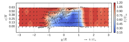
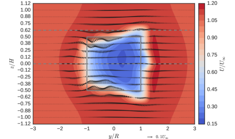
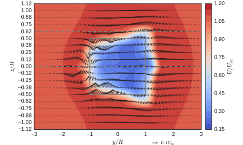
IV.2.1 Mean velocity in three dimensions
In order to visualize the mean velocity field, vector arrows for the mean cross-stream and vertical components are superimposed on top of contours of the streamwise component at in Figure 10. Both CFD models predict the general structure of the mean velocity well, though the SA case has a slightly larger vertical mean flow component, which could be due to stronger tip vortex generation, or lower diffusivity compared with the SST model.
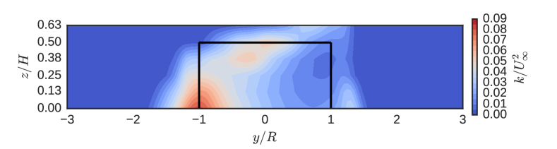
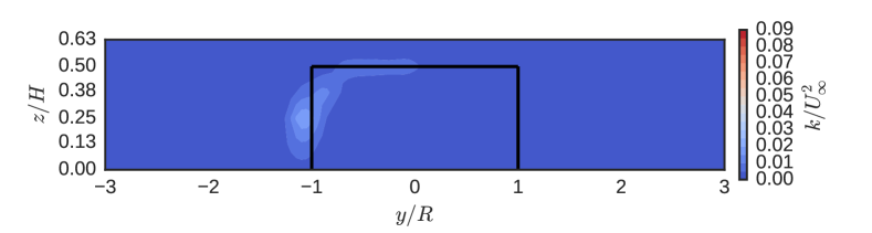
IV.2.2 Turbulence kinetic energy contours
Turbulence kinetic energy contours for the experimental measurements and each CFD case at are presented in Figure 11. As seen in the profiles in Figure 9, the SA model was not able to resolve the majority of the unsteadiness in the flow. In contrast, the SST model did a good job predicting the locations and magnitudes of various peaks in . These are generated along the top of the turbine via tip vortex shedding, and the side of the turbine via dynamic stall. We do however see the smearing effect from the dynamic stall vortex centered around , which is likely more of an issue with wake evolution rather than wake generation.

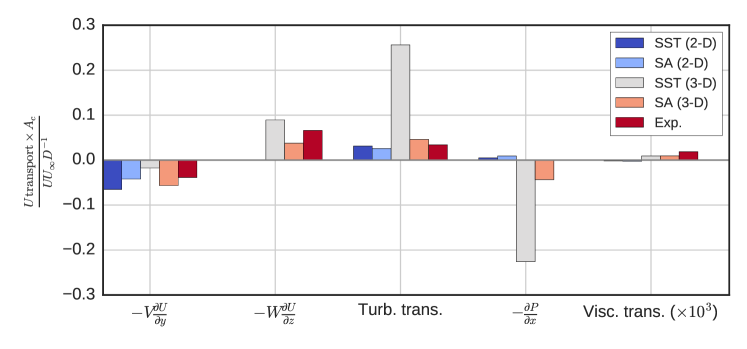
IV.2.3 Momentum recovery
To get an overall idea of the wake recovery predicted by each model, we rearrange the streamwise component of the Navier–Stokes equation to isolate —following Bachant and Wosnik Bachant and Wosnik (2015)—and compute each term at to compare with the experimental results.
We use the RANS models’ eddy viscosity to calculate the turbulent transport via
| (2) |
which is a different approach from those taken on the experiments, where Reynolds stresses were measured, but -derivatives were not:
| (3) |
As such, we should not be surprised if the CFD models predict higher levels of turbulent transport than the experiments.
Normalized weighted averages for each recovery term at are computed and multiplied by the cross-sectional area of the measurement plane, or the channel width in the 2-D cases. Results are shown in a bar chart in Figure 12. Consistent with the relatively large Reynolds number regime, viscous transport is essentially negligible compared with other mechanisms. Cross-stream advection—or the tendency of streamlines to diverge and reduce the streamwise momentum—produces a negative effect for all cases, though the 3-D SST model predicts significantly lower values. Vertical advection is by definition zero for the 2-D cases. The 3-D cases show varying results—with the SST model overpredicting and SA underpredicting the vertical velocity’s effect on replenishing streamwise momentum.
Turbulent transport and streamwise pressure gradient terms show the largest discrepancy between results. The 3-D SST case, despite doing a good job predicting turbulence kinetic energy, significantly overpredicts the turbulent transport term, while other CFD cases are comparable with the experiment. This seems to be balanced by a large adverse pressure gradient, which is also present to a smaller degree in the 3-D SA case. Interestingly, in contrast, both 2-D CFD cases create a wake where the pressure gradient is acting to slightly accelerate the flow at . Unfortunately, pressure data were not acquired from the experiment, though results from the 3-D delayed detached eddy simulation (DDES) of Boudreau and Dumas Boudreau and Dumas (2015) concur with the adverse pressure gradient condition.
V Conclusions
A cross-flow turbine was modeled using the – SST and Spalart–Allmaras (SA) Reynolds-averaged Navier–Stokes turbulence models to test their abilities to predict turbine performance and near-wake dynamics. It was observed that when modeled in 2-D, the performance is over-predicted compared to the data from the tow tank experiments, which was expected due to omission of blade end effects, support strut drag, and increased blockage. Vertical (or axial) wake dynamics were unresolved in the 2-D model, despite being identified as a significant contributor to streamwise wake recovery, which casts doubt on the 2-D model’s applicability as a tool to study array spacing effects.
The 3-D blade-resolved RANS simulations predicted turbine performance and near-wake quite well, where the SA model results were closest to the experimentally measured performance. The SA model’s effectiveness gives hope for the prospect of replacing some physical modeling with blade-resolved CFD. However, the overprediction of power coefficient by the SST model highlights the level of technological and economic risk involved with CFD. That is to say, the SST model, despite being considered relatively trustworthy in these flow conditions, would overestimate power output by 30%.
Both the SST and SA models did a good job predicting the mean velocity field at one turbine diameter downstream, but the SST model was more effective at predicting turbulence kinetic energy, since it is solved for in the turbulence model equations. Streamwise momentum recovery terms were computed from the CFD results over an entire cross-section of the domain at . Values for transport due to the mean pressure gradient and turbulent fluctuations varied a lot between the two turbulence models. Both models, however, we able to at least qualitatively resolve the vertical velocity field, which will be crucial to predicting the performance of closely spaced CFTs.
The effectiveness at predicting the mean velocity field gives credibility to the prospect of using the computed flow field to extrapolate the experimental results, such that the CFD results can be used as a target for a low-order wake generator or force parameterization. These results may also help develop new tip loss corrections for blade element type models, which currently only exist for axial-flow rotors, since they provide access to the pressure and shear forces over the entire blade surface, which were not measured experimentally. Ultimately, however, the computational cost of 3-D simulations—about 1,000 CPU hours per simulated second (or roughly 10,000 CPU hours per operating point)—may be too expensive to be used for CFT engineering work, especially considering the uncertainty involved compared with physical model studies. Since the 3-D wake results appeared to be only weakly asymmetrical in the – plane about , it may be possible to reduce computing power by only modeling the top half of the rotor and using a symmetry boundary condition at the mid-plane. However, 3-D blade-resolved RANS will likely not be practical for turbine array simulations for quite some time, and until they are, low-order models will need to be developed and improved for this purpose.
Acknowledgements.
The authors acknowledge funding through a National Science Foundation CAREER award (principal investigator Martin Wosnik, NSF 1150797, Energy for Sustainability, program manager Gregory L. Rorrer). The authors also thank Dr. Vincent S. Neary and the Sandia National Laboratories Water Power Program for use of their Red Mesa high performance computing cluster.References
- Sutherland, Berg, and Ashwill (2012) H. J. Sutherland, D. E. Berg, and T. D. Ashwill, “A retrospective of VAWT technology,” Tech. Rep. (Sandia National Laboratories, 2012).
- Paraschivoiu (2002) I. Paraschivoiu, Wind Turbine Design with Emphasis on Darrieus Concept, 1st ed. (Polytechnic International, Montreal, Quebec, Canada, 2002).
- Ocean Renewable Power Company (2012) Ocean Renewable Power Company, “America’s first ocean energy delivered to the grid,” (2012).
- Lott (2015) M. C. Lott, “Eiffel tower going green with two new wind turbines,” http://blogs.scientificamerican.com/plugged-in/eiffel-tower-going-green-with-two-new-wind-turbines/ (2015).
- Paulsen et al. (2011) U. S. Paulsen, T. F. Pedersen, H. A. Madsen, K. Enevoldsen, P. H. Nielsen, J. Hattel, L. Zanne, L. Battisti, A. Brighenti, M. Lacaze, V. Lim, J. W. Heinen, P. A. Berthelsen, S. Carstensen, E.-J. de Ridder, G. van Bussel, and G. Tescione, “Deepwind- an innovative wind turbine concept for offshore,” in Proceedings of EWEA (Brussels, Belgium, 2011).
- Sandia National Laboratories (2012) Sandia National Laboratories, “Offshore use of vertical-axis wind turbines gets closer look,” (2012).
- Dabiri (2011) J. Dabiri, “Potential order-of-magnitude enhancement of wind farm power density via counter-rotating vertical-axis wind turbine arrays,” Journal of Renewable and Sustainable Energy 3, 1–13 (2011).
- Balduzzi et al. (2016) F. Balduzzi, A. Bianchini, R. Maleci, G. Ferrara, and L. Ferrari, “Critical issues in the CFD simulation of Darrieus wind turbines,” Renewable Energy 85, 419–435 (2016).
- Howell et al. (2010) R. Howell, N. Qin, J. Edwards, and N. Durrani, “Wind tunnel and numerical study of a small vertical axis wind turbine,” Renewable Energy 35, 412–422 (2010).
- Menter, Kuntz, and Langtry (2003) F. R. Menter, M. Kuntz, and R. Langtry, “Ten years of industrial experience with the sst turbulence model,” Turbulence, Heat and Mass Transfer 4 (2003).
- Alaimo et al. (2015) A. Alaimo, A. Esposito, A. Messineo, C. Orlando, and D. Tumino, “3D CFD analysis of a vertical axis wind turbine,” Energies 8, 3013–3033 (2015).
- Marsh et al. (2015) P. Marsh, D. Ranmuthugala, I. Penesis, and G. Thomas, “Three-dimensional numerical simulations of straight-bladed vertical axis tidal turbines investigating power output, torque ripple and mounting forces,” Renewable Energy 83, 67–77 (2015).
- Rawlings (2008) G. W. Rawlings, Parametric characterization of an experimental vertical axis hydro turbine, Master’s thesis, University of British Columbia (2008).
- Orlandi et al. (2015) A. Orlandi, M. Collu, S. Zanforlin, and A. Shires, “3D URANS analysis of a vertical axis wind turbine in skewed flows,” J. Wind Eng. Ind. Aerodyn. 147, 77–84 (2015).
- Akins (1989) R. Akins, “Measurement of surface pressure on an operating vertical-axis wind turbine,” Tech. Rep. SAND89-7051 (Sandia National Laboratories, 1989).
- Mertens, van Kuik, and van Bussel (2003) S. Mertens, G. van Kuik, and G. van Bussel, “Performance of an H-Darrieus in the skewed flow on a roof,” Journal of Solar Energy Engineering 125, 443–440 (2003).
- Lam and Peng (2016) H. Lam and H. Peng, “Study of wake characteristics of a vertical axis wind turbine by two- and three-dimensional computational fluid dynamics simulations,” Renewable Energy 90, 386–398 (2016).
- Tescione et al. (2014) G. Tescione, D. Ragni, C. He, C. S. Ferreira, and G.J, “Near wake flow analysis of a vertical axis wind turbine by stereoscopic particle image velocimetery,” Renewable Energy 70, 47–61 (2014).
- Nini et al. (2014) M. Nini, V. Motta, G. Bindolino, and A. Guardone, “Three-dimensional simulation of a complete vertical axis wind turbine using overlapping grids,” Journal of Computational and Applied Mechanics (2014).
- Battisti et al. (2011) L. Battisti, L. Zanne, S. Dell’Anna, V. Dossena, G. Persico, and B. Paradiso, “Aerodynamic measurements on a vertical axis wind turbine in a large scale wind tunnel,” Journal of Energy Resources Technology 133 (2011).
- Boudreau and Dumas (2015) M. Boudreau and G. Dumas, “Wake analysis of various hydrokinetic turbine technologies through numerical simulations,” in Proceedings of AERO 2015 (2015).
- Li et al. (2013) C. Li, S. Zhu, Y. lin Xu, and Y. Xiao, “2.5D large eddy simulation of vertical axis wind turbine in consideration of high angle of attack flow,” Renewable Energy 51, 317–330 (2013).
- McLaren (2011) K. W. McLaren, A Numerical and Experimental Study of Unsteady Loading of High Solidity Vertical Axis Wind Turbines, Ph.D. thesis, McMaster University (2011).
- Araya et al. (2014) D. B. Araya, A. E. Craig, M. Kinzel, and J. O. Dabiri, “Low-order modeling of wind farm aerodynamics using leaky rankine bodies,” Journal of Renewable and Sustainable Energy 6 (2014), 10.1063/1.4905127.
- Goude and Agren (2010) A. Goude and O. Agren, “Numerical simulation of a farm of vertical axis marine current turbines,” in Proceedings of the ASME 2010 29th International Conference on Ocean, Offshore and Arctic Engineering (Shanghai, China, 2010).
- Durrani et al. (2011) N. Durrani, N. Qin, H. Hameed, and S. Khushnood, “2d numerical analysis of a vawt wind farm for different configurations,” in Proceedings of 49th AIAA Aerospace Sciences Meeting including the New Horizons Forum and Aerospace Exposition, AIAA 2011-461 (Orlando, FL, 2011).
- Giorgetti, Pellegrini, and Zanforlin (2015) S. Giorgetti, G. Pellegrini, and S. Zanforlin, “CFD investigation on the aerodynamic interferences between medium-solidity Darrieus vertical axis wind turbines,” Energy Procedia 81, 227–239 (2015).
- Li and Calisal (2010) Y. Li and S. M. Calisal, “Modeling of twin-turbine systems with vertical axis tidal current turbines: Part I—power output,” Ocean Engineering 37, 627–637 (2010).
- Antheaume, Maître, and Achard (2008) S. Antheaume, T. Maître, and J.-L. Achard, “Hydraulic Darrieus turbines efficiency for free fluid flow conditions versus power farms conditions,” Renewable Energy 33, 2186–2198 (2008).
- Bachant and Wosnik (2015) P. Bachant and M. Wosnik, “Characterising the near-wake of a cross-flow turbine,” Journal of Turbulence 16, 392–410 (2015).
- Bachant and Wosnik (2014) P. Bachant and M. Wosnik, “Reynolds number dependence of cross-flow turbine performance and near-wake characteristics,” in Proceedings of the 2nd Marine Energy Technology Symposium METS2014 (Seattle, WA, 2014).
- Bachant and Wosnik (2016a) P. Bachant and M. Wosnik, “Effects of reynolds number on the energy conversion and near-wake dynamics of a high solidity vertical-axis cross-flow turbine,” Energies 9 (2016a), 10.3390/en9020073.
- Bachant and Wosnik (2016b) P. Bachant and M. Wosnik, “UNH-RVAT Reynolds number dependence experiment: Reduced dataset and processing code,” figshare. http://dx.doi.org/10.6084/m9.figshare.1286960 (2016b).
- Menter (1994) F. Menter, “Two-equation eddy-viscosity turbulence models for engineering applications,” AIAA Journal 32, 1598–1605 (1994).
- Spalart and Allmaras (1992) P. Spalart and S. Allmaras, “A one-equation turbulence model for aerodynamic flows,” Tech. Rep. AIAA-92-0439 (American Institute for Aeronautics and Astronautics, 1992).
- Ferreira et al. (2007) C. S. Ferreira, H. Bijl, G. van Bussel, and G. van Kuik, “Simulating dynamic stall in a 2d vawt: Modeling strategy, verification and validation with particle image velocimetry data,” Journal of Physics: Conference Series, The Science of Making Torque from Wind 75, 1–13 (2007).
- Crivellini and D’Alessandro (2014) A. Crivellini and V. D’Alessandro, “Spalart–Allmaras model apparent transition and RANS simulations of laminar separation bubbles on airfoils,” International Journal of Heat and Fluid Flow 47, 70–83 (2014).
- Bachant (2016a) P. Bachant, “UNH-RVAT-2D-OpenFOAM: v1.0.0-SST,” Zenodo. http://dx.doi.org/10.5281/zenodo.47928 (2016a).
- Bachant (2016b) P. Bachant, “UNH-RVAT-2D-OpenFOAM: v1.0.0-SA,” Zenodo. http://dx.doi.org/10.5281/zenodo.47929 (2016b).
- Bachant (2016c) P. Bachant, “UNH-RVAT-3D-OpenFOAM: v1.0.0-SST,” Zenodo. http://dx.doi.org/10.5281/zenodo.47926 (2016c).
- Bachant (2016d) P. Bachant, “UNH-RVAT-3D-OpenFOAM: v1.0.0-SA,” Zenodo. http://dx.doi.org/10.5281/zenodo.47927 (2016d).