Stable dipole solitons and soliton complexes in the nonlinear Schrödinger equation with periodically modulated nonlinearity

Abstract

We develop a general classification of the infinite number of families of solitons and soliton complexes in the one-dimensional Gross-Pitaevskii/nonlinear Schrödinger equation with a nonlinear lattice pseudopotential, i.e., periodically modulated coefficient in front of the cubic term, which takes both positive and negative local values. This model finds direct implementations in atomic Bose-Einstein condensates and nonlinear optics. The most essential finding is the existence of two branches of dipole solitons (DSs), which feature an antisymmetric shape, essentially squeezed into a single cell of the nonlinear lattice. This soliton species was not previously considered in nonlinear lattices. We demonstrate that one branch of the DS family (namely, the one which obeys the Vakhitov-Kolokolov criterion) is stable, while unstable DSs spontaneously transform into stable fundamental solitons (FSs). The results are obtained in numerical and approximate analytical forms, the latter based on the variational approximation. Some stable bound states of FSs are found too.

Periodic (alias lattice) potentials is a well-known ingredient of diverse physical settings represented by the nonlinear Schrödinger/Gross-Pitaevskii equations. The lattice potentials help to create self-trapped modes (solitons) which do not exist otherwise, or stabilize those solitons which are definitely unstable in free space. In particular, the lattice potentials generate the bandgap spectrum in the linearized version of the equation, and adding local cubic nonlinearity gives rise to a great variety of gap solitons and their bound complexes residing in the spectral gaps. On the other hand, an essential extension of the concept of lattice potentials is the introduction of nonlinear pseudopotentials, which are induced by spatially periodic modulation of the coefficient in front of the cubic term. While single-peak fundamental solitons (FSs) in nonlinear potentials were studied in detail, more sophisticated ones, such as narrow antisymmetric dipole solitons (DSs), which essentially reside in a single cell of the nonlinear lattice, were not previously considered in this setting. Their shape is similar to that of the so-called subfundamental species of gap solitons in linear lattices, which have a small stability region. In this work, we first develop a general classification of a potentially infinite number of different types of soliton complexes supported by the nonlinear lattice. For physical applications, the most significant finding is the existence of two branches of the DS family, one of which is entirely stable. Its stability is readily predicted by the celebrated Vakhitov-Kolokolov criterion, while the shape of the branch is qualitatively correctly predicted in an analytical form by means of the variational approximation. In addition to that, it is found that some bound states of FSs are stable too, although a majority of such complexes are unstable.

I Introduction

It is well known that the variety of bright solitons, supported by the balance between the self-focusing nonlinearity and diffraction (in optics) or kinetic energy (in matter waves), can be greatly expanded if a spatially periodic (alias lattice) potential is introduced, in the form of photonic lattices acting on optical waves phot-latt , or optical lattices acting on matter waves in atomic Bose-Einstein condensates (BECs) opt-latt . In particular, periodic potentials make it possible to create gap solitons in media with self-defocusing nonlinearity, due to its interplay with the effective negative mass of collective excitations, see original works Dark -Oberthaler and books JYang ; DPeli . In addition to the fundamental solitons, the analysis addressed patterns such as nonlinear Bloch states Kiv2003 ; BlochW , domain walls DomWalls05 , and gap waves, i.e., broad modes with sharp edges gapwave .

The spectral bandgap structure induced by lattice potentials gives rise to many families of gap solitons, classified by the number of a bandgap in which they reside. Further, the oscillatory shape of fundamental gap solitons opens the way to build various two- and multi-soliton bound states through the effective interaction potential induced by their overlapping tails. The variety of the gap-soliton families include both stable and unstable solutions. A specific possibility, revealed in work Thaw and further analyzed in Refs. sub -China , is the existence of subfundamental solitons (SFSs) in the second finite bandgap (in Ref. China SFSs were called “second-family fundamental gap solitons”). They feature a dipole (antisymmetric) shape, which is squeezed, essentially, into a single cell of the lattice potential. The name “subfundamental” implies that the soliton’s norm (in terms of BEC; or the total power, in terms of optics) is smaller than the norm of a stable fundamental soliton (FS) existing at the same value of the chemical potential (or propagation constant, in the optics model) in the second finite bandgap. SFSs have a small stability region China , while unstable ones spontaneously rearrange into stable FSs belonging to the first finite bandgap. Partial stabilization of SFSs was also demonstrated in a model which includes, in addition to the local nonlinearity, long-range dipole-dipole interactions subDD .

Apart from the linear spatially periodic potentials induced by lattice structures, the formation of solitons may be facilitated by nonlinear-lattice pseudopotentials pseudo , which are induced by spatially periodic modulation of the coefficient in front of the cubic term in the respective Gross-Pitaevskii/nonlinear Schrödinger equation (GPE/NLSE) RMP . This structure can be created in BEC by means of the Feshbach resonance controlled by magnetic or optical fields FR-Randy -FR-Tom . Experimentally, the possibility of the periodic modulation of the nonlinearity on a submicron scale was demonstrated in Ref. experiment-inhom-Feshbach . The spatial profile of the nonlinearity may also be “painted” by a fast moving laser beam painting , or imposed by an optical-flux lattice Cooper . Another approach relies on the use of a magnetic lattice, into which the atomic condensate is loaded magn-latt , or of concentrators of the magnetic field concentrator . In optics, spatial modulation of the Kerr coefficient can be achieved by means of an inhomogeneous density of resonant nonlinearity-enhancing dopants implanted into the waveguide Kip . Alternatively, a spatially periodic distribution of resonance detuning can be superimposed on a uniform dopant density. A review of results for solitons supported by nonlinear lattices was given in Ref. RMP .

In the one-dimensional setting, a generic form of the scaled GPE/NLSE for the mean-field amplitude, $\Psi(x,t)$, including both a linear periodic potential, $U(x)$, and a periodic pseudopotential induced by modulation function $P(x)$, both with period $L$, is HS

$$i\Psi_{t}+\Psi_{xx}-U(x)\Psi+P(x)|\Psi|^{2}\Psi=0.$$ (1)

The prototypical examples of both periodic potentials are provided by functions

$$\left\{U(x),P(x)\right\}=\left\{A_{U},A_{P}\right\}+\left\{B_{U},B_{P}\right\}\cos(2x),$$ (2)

where the period is scaled to be $L=\pi$. Equation (1) is written in terms of BEC; in optics, Eq. (1) models the light propagation in planar waveguides, with transverse coordinate $x$, $t$ being replaced by the propagation distance, $z$. In the former case, the model can be implemented in a cigar-shaped BEC trap with the transverse confinement strength subject to periodic modulation along the axial direction, $x$ De Nicola ; Luca . Similarly, the optics realization is possible in the planar waveguides with the thickness (in direction $y$) subject to the same modulation along $x$. It is also relevant to mention that, while we here consider the simplest cubic form of the local nonlinearity in Eq. (1), strong transverse confinement applied to the BEC with a relatively high atomic density gives rise to the one-dimensional equation with nonpolynomial nonlinearity Luca , which may be a subject for a separate work. It is important for the what follows that Eq. (1) conserves the quantities $N$ and $E$,

$$N=\int_{-\infty}^{\infty}|\Psi|^{2}~{}dx,$$ (3)

$$E=\int\limits_{-\infty}^{+\infty}\left(|\Psi_{x}|^{2}+U(x)|\Psi|^{2}-\frac{1}{2}P(x)|\Psi|^{4}\right)~{}dx$$ (4)

having in BEC context the sence of the number of particles and the energy correspondingly.

The objective of the present work is to generate new types of solitons in the model based on Eq. (1), and identify stable solitons among them. To this end, we develop a procedure which makes it possible to predict an infinite number of different families of stationary soliton solutions (starting from the SF and DS families), by means of a coding technique AlfAvr . Actual results are produced, with the help of numerical calculations, for the model with the pseudopotential only Malomed , i.e., Eq. (1) with $U=0$, where effects produced by the periodic modulation of the nonlinearity are not obscured by the linear-lattice potential. Keeping in mind the prototypical $\cos(2x)$ modulation function in Eq. (2), we assume that $P(x)$ in Eq. (1) is an even $\pi$-periodic function, which takes both positive and negative local values. In particular, while FSs supported by nonlinear lattices have been already studied in detail Malomed , a possibility of the existence and stability of the single-cell DSs in the same setting was not considered previously. We demonstrate that this class of solitons is also supported by the nonlinear lattice. It is composed of two branches, one of which is stable, on the contrary to the chiefly unstable SFS family in the models with linear lattices. Another difference is that the single-cell DSs are not subfundamental, as their norm exceeds that of the SFs existing at the same value of the soliton frequency. We also show that, in addition to the SFs and DSs, there exist a plethora of solitons in the model with periodic pseudopotential. While most of them are unstable, we have found some stable bound states of fundamental solitons.

The rest of the paper is structured as follows. Stationary soliton solutions are produced in Section II. Results of the stability analysis are summarized in Section III. Section IV is focused on the new class of the single-cell DSs, including both numerical results and analytical approximations, based on the variational approximation (VA) and Vakhitov-Kolokolov (VK) Vakh stability criterion. The paper is concluded by Section V.

II Stationary modes

Stationary solutions to Eq. (1) with chemical potential $\omega$ (in the optics model, $-\omega$ is the propagation constant) are sought for in the usual form, $\Psi(t,x)=u(x)\exp\left(-i\omega t\right)$, where $u(x)$ is determined by equation

$$u_{xx}+Q(x)u+P(x)u^{3}=0,\quad Q(x)=\omega-U(x).$$ (5)

Solitons are selected by the localization condition,

$$\lim\limits_{x\rightarrow\pm\infty}u(x)=0,$$ (6)

which implies that the function $u(x)$ is real (see, e.g., Ref. AKS ). Therefore, we focus our attention on real solutions to Eq. (5).

For the analysis of stationary modes we apply the approach developed previously for the usual model, with the uniform nonlinearity and a linear lattice potential, i.e., $P(x)=-1$ and $U(x)$ a bounded periodic function AlfAvr . This approach makes use of the fact that the “most common” solutions of equation

$$u_{xx}+Q(x)u-u^{3}=0$$ (7)

are singular, i.e., they diverge at some finite value of $x=x_{0}$ ($\lim\limits_{x\to x_{0}}u(x)=\infty$), as

$$u(x)\approx\pm\sqrt{2}\left(x-x_{0}\right)^{-1}.$$ (8)

Then, it was shown that, under certain conditions imposed on $Q(x)$, nonsingular solutions can be described using methods of symbolic dynamics. More precisely, under these conditions there exists one-to-one correspondence between all solutions of Eq. (7) and bi-infinite sequences of symbols of some finite alphabet, which are called codes of the solutions.

As shown below, this approach can be extended for Eq. (5), which combines the periodic lattice potential and periodic modulation of the nonlinearity coefficient, that represents the nonlinear-lattice pseudopotential.

II.1 The coding procedure

Assume that $Q(x)$ and $P(x)$ in Eq. (5) are even $\pi$-periodic functions. We call a solution $u(x)$ of Eq.(5) singular if $u(x)$ diverges at finite $x_{0}$ as per Eq. (8). In this case, one may also say that solution $u(x)$ collapses at point $x=x_{0}$.

Define Poincaré map $T:\mathbb{R}^{2}\rightarrow\mathbb{R}^{2}$ associated with Eq.(5) as follows:

$$T\begin{pmatrix}u_{0}\\ u_{0}^{\prime}\end{pmatrix}=\begin{pmatrix}u(\pi)\\ u_{x}(\pi)\end{pmatrix}$$ (9)

where $u(x)$ is a solution of the Cauchy problem for Eq. (5) with initial conditions

$$u(0)=u_{0},\quad u_{x}(0)=u_{0}^{\prime}.$$ (10)

We call an orbit a sequence of points $\{p_{n}\}$, $p_{n}\in\mathbb{R}^{2}$ (the sequence may be finite, infinite or bi-infinite), such that $Tp_{n}=p_{n+1}$.

Define sets $\mathcal{U}_{L}^{+}\in\mathbb{R}^{2}$ and $\mathcal{U}_{L}^{-}\in\mathbb{R}^{2}$, $L>0$ as follows: $p=(u_{0},u_{0}^{\prime})\in\mathcal{U}_{L}^{+}$ if and only if solutions of the Cauchy problem for Eq. (5) with initial conditions (10) does not collapse on interval $[0,L]$. Similarly, we define $\mathcal{U}_{L}^{-}$ as the set of initial conditions $u(0)=u_{0}$, $u_{x}(0)=u_{0}^{\prime}$ such that the corresponding solution of the Cauchy problem for Eq.(5) does not collapse on interval $[-L,0]$. It is easy to show that Poincaré map $T$ is defined only on set $\mathcal{U}_{\pi}^{+}$ and transforms it into $\mathcal{U}_{\pi}^{-}$. Accordingly, inverse map $T^{-1}$ is defined only on $\mathcal{U}_{\pi}^{-}$ and transforms this set into $\mathcal{U}_{\pi}^{+}$.

Next, consider the following sets:

$$\Delta_{0}=\mathcal{U}_{\pi}^{+}\cap\mathcal{U}_{\pi}^{-},$$ (11)

$$\Delta_{n+1}^{+}=T\Delta_{n}^{+}\cap\Delta_{0},\quad n=0,1,\ldots,$$ (12)

$$\Delta_{n+1}^{-}=T^{-1}\Delta_{n}^{-}\cap\Delta_{0},\quad n=0,1,\ldots,$$ (13)

Evidently, $\Delta_{0}$ consists of points that have $T$-image and $T$-pre-image. The following statements are valid:

$$\{p\in\Delta_{n}^{+}\}\quad\Leftrightarrow\quad\{Tp,T^{2}p,\ldots,T^{n}p\in\Delta_{0}\};$$ (14)

$$\{p\in\Delta_{n}^{-}\}\quad\Leftrightarrow\quad\{T^{-1}p,T^{-2}p,\ldots,T^{-n}p\in\Delta_{0}\}.$$ (15)

Sets $\Delta_{n}^{\pm}$ are nested in the following sense:

$$\ldots\subset\Delta_{n+1}^{+}\subset\Delta_{n}^{+}\ldots\subset\Delta_{1}^{+}\subset\Delta_{0}$$ (16)

$$\ldots\subset\Delta_{n+1}^{-}\subset\Delta_{n}^{-}\ldots\subset\Delta_{1}^{-}\subset\Delta_{0}.$$ (17)

Now, we define sets

$$\Delta^{+}=\bigcap_{n=1}^{\infty}\Delta_{n}^{+},\quad\Delta^{-}=\bigcap_{n=1}^{\infty}\Delta_{n}^{-}.$$ (18)

Consider set $\Delta=\Delta^{+}\cap\Delta^{-}$. It is is invariant with respect to the action of the $T$ map. Orbits generated by points from $\Delta$ are in one-to-one correspondence with non-collapsing solutions of Eq. (5). Therefore, the numerical study of sets $\Delta_{n}^{\pm}$ allows one to predict and compute bounded solutions of Eq. (5).

There are several restrictions for $Q(x)$ and $P(x)$ for this approach to be applicable. In Ref. AlfLeb , the following statements were proved.

Theorem 1.

Suppose that $Q(x),P(x)\in C^{1}(\mathbb{R})$ and for each $x\in\mathbb{R}$

• there exists ${\widetilde{P}}$ such that $P(x)>0$, $|P^{\prime}(x)|\leq\widetilde{P}$;

• there exist $Q_{0},\widetilde{Q}$, such that $Q(x)\geq Q_{0}$, $|Q^{\prime}(x)|\leq\widetilde{Q}$;

then the solution to the Cauchy problem for Eq.(5) with arbitrary initial conditions (10) can be continued onto the whole real axis $\mathbb{R}$.

Theorem 2.

Suppose that $\forall{x\in\mathbb{R}}$ conditions $P(x)<0$, $Q(x)<0$ holds, then all solutions of Eq. (5) are singular, except the trivial zero solution.

In particular, this implies that, if $P(x)$ and $Q(x)$ are bounded and periodic, and $P(x)>0$ for all $x\in\mathbb{R}$, then all solutions of Eq. (5) are non-singular, and the present approach cannot be applied. In the case of $P(x)<0$, $Q(x)<0$, Eq. (5) has no non-singular solutions, except for the zero state, therefore the approach cannot be used either. However, it follows from Proposition 2 of Ref. AlfLeb that, if $P(x)$ is a sign-alternating function, the collapsing behavior is generic for solutions of Eq. (5), and the application of the approach is reasonable for finding non-collapsing solutions.

In Ref. AlfAvr the case of $P(x)=-1$ in Eq. (5) was considered from a more abstract viewpoint. It was shown that if

• the $\Delta_{0}$ set consist of a finite number $N$ of connected components, $\Delta_{0}=\bigcup_{k=1}^{N}D_{k}$, and each of the components $D_{k}$ is a curvilinear quadrangle, whose boundaries satisfy special conditions of smoothness and monotonicity;

• all the sets $TD_{k}\cap D_{m}$ and $T^{-1}D_{k}\cap D_{m}$, $k,m=1,\dots,N$, are non-empty, and the action of $T$ on curves lying in $D_{k}$ preserves the monotony property;

• areas of sets $\Delta_{n}^{\pm}$ vanish at $n\rightarrow\infty$;

then orbits of the Poincaré map $T$ acting on the $\Delta_{0}$ set are in one-to-one correspondence with bi-infinite sequences of symbols of some $N$-symbol alphabet.

This result can be commented as follows. Let symbols of the alphabet be the numbers $1,\dots,N$. Denote the connected components of $\Delta_{0}$ by $D_{k}$, $k=1,\ldots,N$. Then for each non-collapsing solution $u(x)$ there exist an unique orbit $\{p_{k}\}$, $k=0,\pm 1,\pm 2,\ldots$, $p_{k}\in\Delta$, and the corresponding unique bi-infinite sequence $\ldots\alpha_{-1},\alpha_{0},\alpha_{1},\ldots$, $\alpha_{k}\in\{1,\ldots,N\}$ such that

$$\ldots,~{} p_{-1}=T^{-1}p_{0}\in D_{\alpha_{-1}},\quad p_{0}\in D_{\alpha_{0}},$$ (19)

$$p_{1}=Tp_{0}\in D_{\alpha_{1}},\ldots$$

On the contrary, for each bi-infinite sequence of numbers $\{1,\ldots,N\}$ there exists an unique orbit $\{p_{k}\}$, $k=0,\pm 1,\pm 2,\ldots$, $p_{k}\in\Delta$, that satisfies condition (19) and corresponds to an unique solution $u(x)$. The check of conditions (a),(b) and (c) was carried out in Ref. AlfAvr numerically, using some auxiliary statements.

In what follows below, we apply this approach to Eq. (5) with $U(x)=0$, i.e., $Q(x)=\omega$, when the linear potential is absent, and only the pseudopotential is present in Eq. (5), induced by the modulation function taken as

$$P(x)=\alpha+\cos(2x),$$ (20)

This is a new setting for which the present method was not elaborated previously.

II.2 Numerical results

According to what was said above [Eq. (20)], we now focus on the following version of Eq. (5):

$$u_{xx}+\omega u+(\alpha+\cos 2x)u^{3}=0.$$ (21)

Due to Theorem 1 we impose restriction $\alpha\in(-1,1)$ in Eq. (21) for the approach to be applied, i.e., the nonlinearity coefficient (20) must be a sign-changing function of $x$. Another restriction, $\omega<0$, comes from the obvious condition of the soliton localization, given by Eq. (6).

Sets $\mathcal{U}_{\pi}^{\pm}$. The set $\mathcal{U}_{\pi}^{+}$ was found by scanning the plane $(u,u^{\prime})$ of initial data by means of the following procedure. The Cauchy problem for Eq. (21) was solved numerically, taking as initial conditions $u(0)=n\Delta u$, $u_{x}(0)=m\Delta u^{\prime}$, $m,n=-L,\ldots,L$ where spacings $\Delta u$ and $\Delta u^{\prime}$ are small enough (typical values were $\Delta u=\Delta u^{\prime}=0.01$). If the absolute value of the solution of the Cauchy problem exceeds, in interval $[0;\pi]$, some sufficiently large value $u_{\infty}$, it is assumed that the collapse occurs. The corresponding point is marked white, otherwise, it is grey. The computations were actually performed for $u_{\infty}=10^{5}$ and further checked for $u_{\infty}=10^{7}$, the results obtained for both cases agreeing very well. Since Eq.(21) is invariant with respect to inversion $x\to-x$, the set $\mathcal{U}_{\pi}^{-}$ is the reflection of $\mathcal{U}_{\pi}^{+}$ with respect to the $u$-axis. The numerical results allow us to conjecture that, for $\alpha\in(-1;1)$, $\mathcal{U}_{\pi}^{\pm}$ are unbounded spirals with infinite number of rotations around the origin, see Fig. 1.

Set $\Delta_{0}$. Some examples of set $\Delta_{0}$ are displayed in Fig. 1. Panel (A) of Fig. 1 corresponds to the case of $\omega=-1$, $\alpha=-1.1$, when $\Delta_{0}$ consists of only one connected component situated in the origin. This fact agrees with Theorem 2. If $\alpha\in(-1;1)$, then, presumably, $\Delta_{0}$ is unbounded and consists of an infinite number of connected components that are situated along the $u$ and $u^{\prime}$ axes [panels (B)-(F) of Fig. 1]. The connected components can be enumerated by symbols $\{A_{k}\},k=\pm 1,\pm 2,\dots$ (the components along $u$ axis) and $\{B_{k}\},k=\pm 1,\pm 2,\dots$ (the components along $u^{\prime}$ axis). The central connected component is denoted $O$.

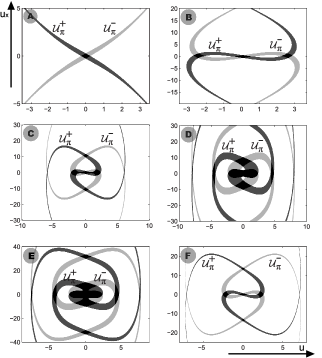
Figure 1: $\mathcal{U}_{\pi}^{+}$ (dark grey color), $\mathcal{U}_{\pi}^{-}$ (light grey color) and their intersection $\Delta_{0}$ (black color) in the model based on Eq. (21), at different values of parameters $\omega$ and $\alpha$: A) $\omega=-1$, $\alpha=-1.1$; B) $\omega=-1$, $\alpha=-0.3$; C) $\omega=-1$, $\alpha=0.15$; D) $\omega=-1$, $\alpha=0.5$; E) $\omega=-0.7$, $\alpha=0.55$; F) $\omega=-1.5$, $\alpha=0$.

The basic assumption for the applicability of the coding approach is that the the connected components are curvilinear quadrangles with opposite sides lying on the boundaries of $\mathcal{U}_{\pi}^{+}$ and $\mathcal{U}_{\pi}^{-}$. Due to geometric properties of the spirals, it is quite natural to assume that all connected components $\{A_{k}\},\{B_{k}\},k=\pm 1,\pm 2,\dots$ satisfy this condition. However, central connected component $O$ may be such a curvilinear quadrangle (cases A, B, F in Fig. 1), or may be not (cases C, D, E in Fig. 1), depending on values of $\omega$ and $\alpha$.

Coding. Assume that the parameters $\omega$ and $\alpha$ are such that all connected components in $\Delta_{0}$ are curvilinear quadrangles. Then, our numerical study indicates that $T^{-1}A_{k}$, $T^{-1}B_{k}$, $k=1,2,\ldots$, and $T^{-1}O$ are infinite curvilinear strips situated inside $\mathcal{U}_{\pi}^{+}$ and crossing all the connected components. Similarly, $TA_{k}$, $TB_{k}$, $k=1,2,\ldots$, and $TO$ are also curvilinear strips situated inside the $\mathcal{U}_{\pi}^{-}$ set, that also cross all the connected components. $T$-pre-images of the sets

$$T^{-1}Z\cap A_{l},\quad T^{-1}Z\cap B_{l},\quad T^{-1}Z\cap O,\quad l=\pm 1,\pm 2,\ldots,$$

$$Z\in\{O,A_{k},B_{k},k=\pm 1,\pm 2,\ldots\},$$

are infinite curvilinear strips belonging to $T^{-1}Z$. Similar statement are also valid for $T$-images of $TZ\cap A_{l}$, $TZ\cap B_{l}$, $TZ\cap O$ $l=\pm 1,\pm 2,\ldots$ which are placed inside $TZ$, with $Z\in\{O,A_{k},B_{k},k=\pm 1,\pm 2,\ldots\}$. Therefore the situation is similar to one considered in Ref.AlfAvr and we conjecture that the dynamics of $T$ is similar to dynamics of the Poincaré map from Ref.AlfAvr , and that there is one-to-one correspondence between all nonsingular solutions of Eq.(21) and bi-infinite sequences $\{\ldots Z_{-1},Z_{0},Z_{1},\ldots\}$ based on the infinite alphabet of symbols $Z_{m}\in\{O,A_{k},B_{k},k=\pm 1,\pm 2,\ldots\}$. The orbit corresponding to code $\{\ldots,Z_{-1},Z_{0},Z_{1},\ldots\}$ visits successively connected components $Z_{m}$, $m=\ldots,-1,0,1,\ldots$. Note that the orbit corresponding to the soliton solution starts and ends in the central connected component, therefore it has the code of the form $\{\ldots,O,O,Z_{1},Z_{2},\ldots,Z_{N},O,O,\ldots\}$ where symbols $Z_{1}$ and $Z_{N}$ are different from $O$.

Solitons. Regardless of whether the coding conjecture is true or false generically, it might be used for the prediction of possible shapes of nonlinear modes. Specifically, the location of the connected components in the plane of $(u,u^{\prime})$, and the order in which the orbit visits them, yields comprehensive information about the nonlinear mode. In the present model, the predicted nonlinear modes were found numerically in all the cases considered. Some of soliton solutions of Eq.(21) and their codes are shown in Fig. 2 for $\omega=-1$, $\alpha=-0.1$. The soliton in panel (B) is the FS, cf. Ref. Malomed , with code $\{\dots,O,A_{1},O,\dots\}$, or $\{\dots,O,A_{-1},O,\dots\}$, which is its symmetric counterpart. Another particular solution, shown in panel G, represents the above-mentioned DSs (dipole solitons), which are essentially confined to a single cell of the nonlinear lattice. This solution corresponds to code $\{\dots,O,B_{-1},O,\dots,\}$, and its symmetric counterpart is $\{\dots,O,B_{1},O,\dots\}$. The DSs are similar to the (mostly unstable) SFSs reported in Refs. Thaw -China in models with the linear lattice potential, as both soliton species feature the antisymmetric profile squeezed into a single cell of the underlying lattice (the linear one, in the case of the SFSs, and the nonlinear lattice, as concerns the DSs). The area of the localization of the soliton corresponding to code $\{\ldots,O,Z_{1},Z_{2},\ldots,Z_{N},O,\ldots\}$, where the symbols $Z_{1}$ and $Z_{N}$ are different from $O$, is $N\pi$, i.e., it extends over $N$ periods of the underlying nonlinear lattice. In particular, the solitons with codes $\{\ldots,O,O,Z,O,O,\ldots\}$, $Z\neq O$ (named elementary solitons in what follows below), are localized, essentially, in one period of the lattice.

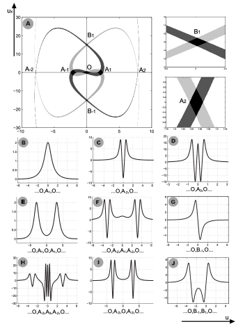
Figure 2: Numerically found solutions of Eq. (21) and their codes for parameters $\omega=-1$, $\alpha=-0.1$; A) $\mathcal{U}_{\pi}^{\pm}$ sets; B)-J) the profiles of solitons together with their codes

III The linear-stability analysis

As said above, stability is a critically important issue for solitons supported by lattice potentials. Here, we address the stability of solitons produced by Eqs. (1), (21). It has been shown in Sect. II that there exist a great variety of shapes of such modes. Thus, adopting the nonlinear lattice as given by Eq. (20), we aim to study the linear stability of solitons generated by equation

$$i\Psi_{t}+\Psi_{xx}+(\alpha+\cos 2x)|\Psi|^{2}\Psi=0$$ (22)

Following the well-established approach, (see, e.g., Ref. JYang ), we consider small perturbations around a stationary solution $\Psi_{0}(x,t)=u(x)e^{-i\omega t}$ in the form of

$$\Psi(t,x)=\left[u(x)+\widetilde{U}(t,x)\right]e^{-i\omega t},~{}\left|\widetilde{U}(t,x)\right|\ll 1,$$ (23)

where $u(x)$ is a localized solution of Eq. (21), and the perturbation satisfies the linear equation

$$i\widetilde{U}_{t}+\widetilde{U}_{xx}+\omega\widetilde{U}+(\alpha+\cos 2x)u^{2}(2\widetilde{U}+\widetilde{U}^{\ast})=0,$$ (24)

where asterisk means complex conjugate. Seeking solutions to Eq. (24) as

$$\widetilde{U}(t,x)=(v(x)+w(x))e^{\lambda t}+(v^{\ast}(x)-w^{\ast}(x))e^{\lambda^{\ast}t},$$ (25)

we arrive at the eigenvalue problem

$$LY=\lambda Y,$$ (26)

$$L=i\begin{pmatrix}0&L_{0}\\ L_{1}&0\end{pmatrix},~{}~{}~{}Y=\begin{pmatrix}v\\ w\end{pmatrix},$$ (27)

where

$$L_{0}=\partial_{xx}+G_{0}(x),\quad G_{0}(x)=\omega+(\alpha+\cos 2x)u^{2},$$

$$L_{1}=\partial_{xx}+G_{1}(x),\quad G_{1}(x)=\omega+3(\alpha+\cos 2x)u^{2}.$$

The soliton is linearly unstable if the spectrum produced by Eq. (26) contains at least one eigenvalue $\lambda$ with a non-zero real part, $\Re(\lambda)>0$. Otherwise, the solitons are linearly stable.

Equation (26) generates the spectrum consisting of continuous and discrete parts. It is easy to show that the continuous spectrum is represented by two rays, $[-i\omega;+i\infty)$ and $(-i\infty;i\omega]$, if $\omega<0$, and by the whole imaginary axis, if $\omega>0$. The discrete spectrum includes zero eigenvalue $\lambda=0$. Other eigenvalues of the discrete spectrum appear in quadruples, since if $\lambda$ is an eigenvalue then $-\lambda$, $\lambda^{\ast}$ and $-\lambda^{\ast}$ are eigenvalues too.

To find discrete eigenvalues numerically, the Fourier Collocation Method (FCM) JYang was used. This method is very efficient to find exponential instabilities, that appears due to real eigenvalues. However it is known that it can miss the situations of weak oscillatory instabilities caused by quartets of complex eigenvalues with small real parts (see e.g. Egor ) where more sophisticated methods, such as Evans function method, PelKiv , must be applied. With the help of FCM, a great number of stationary solutions of Eq.(22), represented by different codes, were analyzed. Due the infinite number of essentially different solutions, it is not possible to perform a comprehensive stability analysis of all localized solutions, even of all elementary solitons. However, we observed that a majority of the solitons are linearly unstable, thus being physically irrelevant solutions. Stable solitons can be categorized as follows:

a) Among the elementary solitons, it was found that FS and DS are linearly stable, under some restrictions on $\omega$ and $\alpha$. Other elementary solitons were found to be unstable. Note that FSs are considered as stable solutions in models with linear lattice potentials, see Ref. Malomed and references therein, while the SFSs are chiefly unstable in that case, having a small stability region China (strictly speaking, FSs in models with linear lattice potentials may also feature a very weak oscillatory instability, having at the same time great lifetime, see Egor ). Therefore, stable DSs supported by the nonlinear pseudopotential, whose shape is very similar to that of the chiefly unstable SFSs in the systems with linear lattice potentials, deserve a detailed consideration, which is given in Sect. IV. It includes not only numerical results, but also analytical ones based on VA.

b) There are stable bound states of FSs – for instance, with codes $\{\dots,O,A_{1},A_{-1},A_{1},O,\dots\}$, $\{\dots,O,A_{1},O,A_{-1},O,\dots\}$. However, other bound states of these modes may be unstable.

Stability spectra for some solitons and their bound states are shown in Fig.3. These example adequately represent the generic situation.

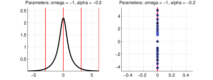
(a)

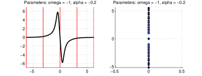
(b)

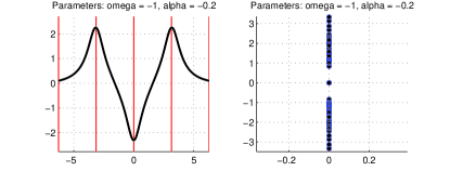
(c)

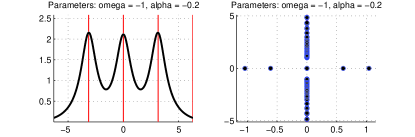
(d)

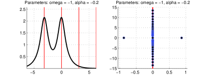
(e)

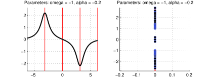
(f)

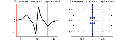
(g)

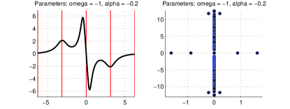
(h)

Figure 3: Localized solutions, their codes, and linear-stability spectra for $\omega=-1$, $\alpha=-0.2$.

IV Dipole solitons (DSs)

IV.1 The variational approximation

Some general features of soliton solutions of Eq. (21) can be obtained by means of the VA, using the fact that Eq. (21) for the stationary states can be derived from Lagrangian

$$L=\int_{-\infty}^{+\infty}\left\{\frac{1}{2}\left(u^{\prime}\right)^{2}-\frac{1}{2}\omega u^{2}-\frac{1}{4}\left[\alpha+\cos\left(2x\right)\right]u^{4}\right\}~{}dx.$$ (28)

In Ref. Malomed , VA was successfully applied for analysis of FS. In that study, the soliton was assumed to be bell-shaped, and the following ansatz was used

$$u(x)=A\exp\left(-\frac{x^{2}}{2W^{2}}\right),$$ (29)

The VA had yielded correct predictions for the existence of the minimal norm

$$N=\int_{-\infty}^{+\infty}u^{2}(x)dx=\sqrt{\pi}A^{2}W.$$ (30)

for the FS, and the existence of an amplitude threshold for stable solitons.

A similar analysis for the DS may be based on the simplest spatially odd ansatz:

$$u(x)=Ax\exp\left(-\frac{x^{2}}{2W^{2}}\right),$$ (31)

The maximum value of $u(x)$, which is $\sqrt{e}AW$, is situated at $x_{\max}=W$, therefore $W$ may be regarded as the half-width of the DS. Norm $N$ of ansatz (31) is

$$N=\frac{\sqrt{\pi}}{2}A^{2}W^{3}.$$ (32)

Equation (32) makes it possible to eliminate the amplitude $A$ in favor of the norm:

$$A^{2}=\frac{2}{\sqrt{\pi}}\frac{N}{W^{3}}.$$ (33)

The substitution of ansatz (31) into Lagrangian (28) and calculation of the integrals yields the following effective Lagrangian:

$$L_{\mathrm{eff}}=-\frac{\omega}{2}N+\frac{3N}{4W^{2}}-\frac{3\alpha N^{2}}{16\sqrt{2\pi}W}-$$

$$-\frac{N^{2}e^{-W^{2}/2}}{16\sqrt{2\pi}W}\left(3-6W^{2}+W^{4}\right),$$ (34)

where Eq. (33) was used to eliminate $A^{2}$. The Euler-Lagrange (variational) equations following from the effective Lagrangian are

$$\partial L_{\mathrm{eff}}/\partial W = 0,$$ (35)

$$\partial L_{\mathrm{eff}}/\partial N = 0,$$ (36)

with $W$ and $N$ treated as free variational parameters for given $\omega$.

Hereafter, we consider the case $\alpha=0$ in more detail. Equation (35) implies the following relation between $N$ and $W$:

$$N=\frac{48\sqrt{\pi/2}\exp\left(W^{2}/2\right)}{W\left(3+9W^{2}-9W^{4}+W^{6}\right)}.$$ (37)

This relation is plotted in Fig. 4, (left panel, thin dashed line), where it attains a minimum value,

$$N_{\min}^{(\mathrm{VA})}\approx 19.41$$ (38)

at $W=W_{0}\approx 0.806$.

An essential feature of the dependence is that it predicts the existence of a minimum norm necessary for the DS to exist. Furthermore, it follows from Eq.(37) that the range of the variation of $W$ predicted by the VA is finite:

$$0<W<W^{*}_{VA}\approx 1.21.$$ (39)

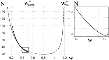
Figure 4: Left panel: the relation between the norm and width of the DS, as predicted by the variational approximation, (thin dashed line, $\alpha=0$). Bold line shows the same relation for numerically computed DS. Right panel: the magnification of the bold line in small rectangle in the left panel

The second variational equation, Eq.(36), yields, after additional algebraic manipulations, a monotonic dependence $\omega$ on $W$:

$$\omega=\frac{3}{2}\cdot\frac{-9+33W^{2}-13W^{4}+W^{6}}{W^{2}\left(3+9W^{2}-9W^{4}+W^{6}\right)}.$$ (40)

It may be combined with Eq. (37) to apply the VK stability criterion Vakh , $dN/d\omega\equiv\left(d\omega/dW\right)^{-1}dN/dW<0$. Because it follows from Eq. (40) that $d\omega/dW$ is always positive, the VK criterion predicts that stable is the left branch in Fig. 4, with $dN/dW<0$, which corresponds to interval

$$0<W<W_{0}\approx 0.806,$$ (41)

while the right branch, with $dN/dW>0$, i.e., $W>W_{0}$ is unstable.

Note that Eq. (40) is compatible with the above-mentioned localization condition, $\omega<0$, at $0<W<0.556$, while the fact that the VA predicts $\omega>0$ at $W>0.556$ is a manifestation of its inaccuracy. It is worthy to note that the predicted stability region tends to have $\omega<0$, i.e., the stability is predicted in the region where the VA is more accurate.

To summarize, the predictions of VA are:

(i) the existence of the minimal norm of the DS;

(ii) the existence of its maximum width;

(iii) the existence of the maximum width of DSs to be stable.

In what follows below we show that these predictions qualitatively agree with results of numerical computation. The application of the VA to more complex solitons is much more cumbersome and is not presented here.

IV.2 Numerical results for stationary dipole solitons

The numerical computation of DS profiles was carried out by dint of the shooting method. The results can be summarized as follows.

(1) The DS family of may be parameterized by $\omega$ or by $W$, which is here defined as the distance of maxima of the wave field from the central point. The amplitude and norm of the DS grow as the soliton shrinks (i.e., when $W$ tends to zero), and in this limit $\omega$ tends to $-\infty$. Examples of DS profiles for $\alpha=0$ and $\omega=-15$ (thin line), $\omega=-7$ (dash line), and $\omega=-1$ (thick line) are depicted in Fig. 5. The dependence of norm $N$ on $W$ is also shown in Fig. 4 (bold line in the left panel and the right panel). It is seen in Fig. 4 that this dependence agrees well with VA results at the interval left to $W_{\rm comp}^{*}$, the maximum width of DS. Also it follows from Fig. 4 that there is a minimum norm $N_{\min}$ necessary for the existence of the DS, hence the above-mentioned prediction (i) of the VA holds.

(2) The DS exists for $\omega<\omega^{\ast}$. At $\omega=\omega^{\ast}\approx 0.265$ , the DS family, coded by $\{\ldots,O,B_{\pm 1},O,\ldots,\}$, undergoes a saddle-node bifurcation and annihilates with the family coded by $\{\dots,O,A_{\mp 1},B_{\pm 1},A_{\pm 1},O,\dots\}$ (see Fig. 6). This implies that width $W$ of the DSs is bounded from above, hence prediction (ii) of VA, concerning the existence of the maximum width of the DS, holds too. However the estimation of VA for the greatest width of the dipol soliton, $W_{VA}^{*}$, is quite rough when compared with computed value $W_{\rm comp}^{*}$, see Fig. 4.

Note that the panel A in Fig. 6 also demonstrates that, although the single-cell DS is very similar, in its shape, to the SFS in systems with linear lattice potentials, the DS in the present model is not subfundamental, as its norm is higher than that of the FS existing at the same $\omega$. The panel B of Fig. 6 presents the dependence of energy $E$ versus the norm $N$. It follows from Fig. 6 that the energy for the branch coded by $\{\dots,O,A_{\mp 1},B_{\pm 1},A_{\pm 1},O,\dots\}$ is greater than the energy of the DS branch.

Thus, the predictions of the VA qualitatively agree with the numerical results, although the accuracy of the VA is rather low, as ansatz (31) is not accurate enough. For instance, the VA-predicted minimum norm, given by Eq. (38), is smaller than the respective numerical value,

$$N_{\min}^{\mathrm{(num)}}\approx 27.5,$$ (42)

by $\approx 30\%$. The ansatz may be improved by adding more terms to it, but then the VA becomes too cumbersome.

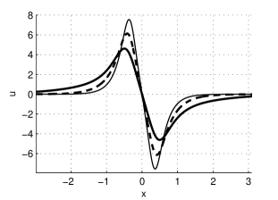
Figure 5: Numerically found profiles of the dipole solitons for $\omega=-15$ (thin line), $\omega=-7$ (dash line), and $\omega=-1$ (thick line), with $\alpha=0$ in Eq. (21).

IV.3 Evolution of dipole solitons

To check the above-mentioned prediction (iii) of the VA concerning the stability of the DSs, we have performed simulations of the evolution of these solitons in the framework of Eq. (1), with $U(x)=0$ and $P(x)$ corresponding to Eq. (21). The simulations were run by means of the Trofimov-Peskov finite-difference numerical scheme Trofimov . The scheme is implicit, its realization implying iterations for the calculation of values in each temporal layer, but it allows running computation with larger temporal steps. In order to reveal instability (if it is), the soliton profile was perturbed in initial moment with small spatial perturbation. A finite spatial domain $[-4\pi,4\pi]$ was used, with reflection of radiation from boundaries eliminated by means of absorbing boundary conditions.

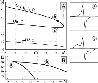
Figure 6: A: The bifurcation diagram for solitons in Eq. (21) with $\alpha=0$: the family of single-cell dipole solitons corresponding to code $\{\ldots,O,B_{\pm 1},O,\ldots\}$ coalesces at $\omega=\omega^{\ast}$ with family $\{\dots,O,A_{\mp 1},B_{\pm 1},A_{\pm 1},O,\dots\}$. The bottom branch (dashed line) represents fundamental solitons, showing that, on the contrary to the SFSs in models with linear lattice potentials, the norm of the dipole solitons is higher than the norm of the fundamental solitons at the same value of $\omega$. B: Dependence of the energy $E$ on $N$ for the dipole-soliton branch. Two profiles of solitons coexisting at $\omega=-0.8$ are displayed in the right panels (a) and (b), the corresponding points are marked in panels A and B

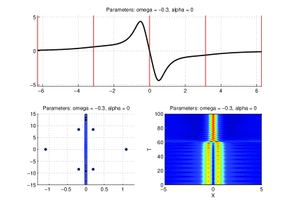
(a)

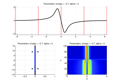
(b)

(c)

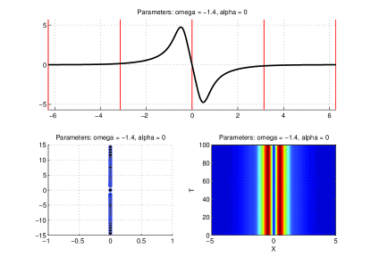
(d)

Figure 7: Typical examples of dipole solitons, their linear-stability spectra, and unstable and stable temporal evolution, for $\alpha=0$ in Eq. (21). Additional examples of the evolution are shown below in the lower panel of Fig. 8.

Typical results of the simulations are presented in Fig. 7, for $\alpha=0$ in Eq. (21). One can conclude that the VA prediction (iii), based on the VK criterion, is generally valid. The results are summarized in the $\left(\omega,N\right)$ plane, as shown in Fig. 8. The DS is stable for the values of omega corresponding to the slope of the $N(\omega)$ curve situated left to the minimum point $\omega_{\min}\approx-0.66$ and transforms into FS at the slope right to this point. The border between the stability and instability regions in the top panel of Fig. 8 is fuzzy. Within this “fuzzy area” the evolution of initial DS profile strongly depends on the type of imposed perturbation and parameters of the numerical method.

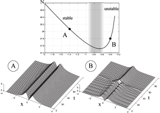
Figure 8: The upper panel: the $N(\omega)$ curve for the dipole solitons at $\alpha=0$ in Eq. (21). The lower panel displays typical examples of the stable and unstable evolution of the dipole solitons for $\omega=-1.4$ and $\omega=-0.4$, respectively. In the latter case, the unstable dipole soliton transforms into a fundamental soliton corresponding to $\omega\approx-13.96$ and amplitude $\approx 5.43$. In “fuzzy area” the simulation is very sensitive to the type of initial perturbation and the parameters of the numerical method.

V Conclusion

The mathematical issue considered in this work is the classification of families of solitons and their bound states in the model of the nonlinear lattice, which is represented by the periodically varying nonlinearity coefficient. A condition necessary for the existence of the infinite variety of the bound states is that the local coefficient must assume both positive and negative values. Then, the analysis is performed for the physically relevant problem, which may find direct applications to Bose-Einstein condensates and planar waveguides in nonlinear optics: finding two branches of the DSs (dipole solitons), whose antisymmetric profile is confined, essentially, to a single cell of the nonlinear lattice. The shape of these solitons is very similar to that of the subfundamental solitons, which are known in models with usual linear lattice potentials, where they are chiefly unstable. An essential finding reported here is that one of two branches of the single-cell DS, family which satisfies the VK (Vakhitov-Kolokolov) criterion, is completely stable. Also it was found that DSs belonging to the unstable branch evolve into stable FSs. These results were obtained by means of numerical methods and also, in a qualitatively correct form, with the help of the VA (variational approximation). Besides that, it was found that particular species of FS bound states are stable too.

References

- (1) N. K. Efremidis, S. Sears, D. N. Christodoulides, J. W. Fleischer, and M. Segev, Phys. Rev. E 66, 046602 (2002); Y. V. Kartashov, V. A. Vysloukh, and L. Torner, Prog. Opt. 52, 63 (2009).
- (2) V. A. Brazhnyi and V. V. Konotop, Mod. Phys. Lett. B 18, 627 (2004); O. Morsch and M. Oberthaler, Rev. Mod. Phys. 78, 179 (2006).
- (3) V. V. Konotop, M. Salerno, Phys. Rev. A 65 021602 (2002) .
- (4) G. L. Alfimov, V. V. Konotop and M. Salerno, Europhys. Lett. 58 7-13 (2002).
- (5) K. M. Hilligsoe, M. K. Oberthaler, and K. P. Marzlin, Phys. Rev. A 66, 063605 (2002).
- (6) P. J. Y. Louis, E. A. Ostrovskaya, C. M. Savage and Yu. S. Kivshar, Phys. Rev. A 67 013602 (2003) .
- (7) H. Sakaguchi and B. A. Malomed, J. Phys. B 37, 1443-1459 (2004).
- (8) D. E. Pelinovsky, A. A. Sukhorukov and Yu. S. Kivshar, Phys. Rev. E 70 036618 (2004).
- (9) B. Eiermann, Th. Anker, M. Albiez, M. Taglieber, P. Treutlein, K.-P. Marzlin, and M. K. Oberthaler, Phys. Rev. Lett. 92 230401 (2004).
- (10) J. Yang, Nonlinear Waves in Integrable and Nonintegrable Systems (SIAM: Philadelphia, 2010).
- (11) D. E. Pelinovsky, Localization in Periodic Potentials: from Schrödinger Operators to the Gross-Pitaevskii Equation (Cambridge University Press: Cambridge, 2011).
- (12) B. Wu and Q. Niu, Phys. Rev. A 64 061603(R) (2001)
- (13) P. G. Kevrekidis, B. A. Malomed, D. J. Frantzeskakis, A. R. Bishop, H. Nistazakis and R. Carretero-González, Mathematics and Computers in Simulation 69 334-345 (2005).
- (14) Th. Anker, M. Albiez, R. Gati, S. Hunsmann, B. Eiermann, A. Trombettoni, and M. K. Oberthaler, Phys. Rev. Lett. 94, 020403 (2005), Phys. Rev. Lett. 92, 230401 (2004); T. J. Alexander, E. A. Ostrovskaya and Yu. S. Kivshar, ibid.. 96, 040401 (2006).
- (15) T. Mayteevarunyoo and B. A. Malomed, Phys. Rev. A 74, 033616 (2006).
- (16) S. K. Adhikari and B. A. Malomed, EPL 79, 50005 (2007); D. L. Wang, X. H. Yan, and W. M. Liu, Phys. Rev. E 78, 026606 (2008).
- (17) S. K. Adhikari, B. A. Malomed, Physica D 238, 1402-1312 (2009).
- (18) T. Mayteevarunyoo, B. A. Malomed, B. B. Baizakov, and M. Salerno, Physica D 238, 1439-1448 (2009).
- (19) J. Cuevas, B. A. Malomed, P. G. Kevrekidis, and D. J. Frantzeskakis, Phys. Rev. A 79, 053608 (2009).
- (20) Y. Zhang, Z. Liang, and B. Wu, Phys. Rev. A 80, 063815 (2009).
- (21) W. A. Harrison, Pseudopotentials in the Theory of Metals (Benjamin: New York, 1966).
- (22) Y. V. Kartashov, B. A. Malomed, and L. Torner, Rev. Mod. Phys. 83, 247-306 (2011).
- (23) S. E. Pollack, D. Dries, M. Junker, Y. P. Chen, T. A. Corcovilos, and R. G. Hulet, Phys. Rev. Lett. 102, 090402 (2009).
- (24) C. C. Chin, R. Grimm, P. Julienne, and E. Tsienga, Rev. Mod. Phys. 82, 1225 (2010).
- (25) D. M. Bauer, M. Lettner, C. Vo, G. Rempe, and S. Dürr, Nature Phys. 5, 339 (2009); M. Yan, B. J. DeSalvo, B. Ramachandhran, H. Pu, and T. C. Killian, Phys. Rev. Lett. 110, 123201 (2013).
- (26) R. Yamazaki, S. Taie, S. Sugawa, and Y. Takahashi, Phys. Rev. Lett. 105, 050405 (2010).
- (27) K. Henderson, C. Ryu, C. MacCormick, and M. G. Boshier, New J. Phys. 11, 043030 (2009).
- (28) N. R. Cooper, Phys. Rev. Lett. 106, 175301 (2011).
- (29) H. S. Ghanbari, T. D. Kieu, A. Sidorov, and P. Hannaford, J. Phys. B: At. Mol. Opt. Phys. 39, 847 (2006); O. Romero-Isart, C. Navau, A. Sanchez, P. Zoller, and J. I. Cirac, Phys. Rev. Lett. 111, 145304 (2013); S. Ghanbari, A. Abdalrahman, A. Sidorov, and P. Hannaford, J. Phys. B: At. Mol. Opt. Phys. 47, 115301 (2014); S. Jose, P. Surendran, Y. Wang, I. Herrera, L. Krzemien, S. Whitlock, R. McLean, A. Sidorov, and P. Hannaford, Phys. Rev. A 89, 051602 (2014).
- (30) C. Navau, J. Prat-Camps, and A. Sanchez, Phys. Rev. Lett. 109, 263903 (2012).
- (31) J. Hukriede, D. Runde, and D. Kip, J. Phys. D 36, R1 (2003).
- (32) H. Sakaguchi and B. A. Malomed, Phys. Rev. A 81, 013624 (2010).
- (33) S. De Nicola, B. A. Malomed, and R. Fedele. Phys. Lett. A 360, 164-168 (2006).
- (34) L. Salasnich, A. Cetoli, B. A. Malomed, F. Toigo, L. Reatto, Phys. Rev. A 76, 013623 (2007).
- (35) G. L. Alfimov and A. I. Avramenko, Physica D 254, 29 (2013).
- (36) G. Theocharis, P. Schmelcher, P. G. Kevrekidis, and D. J. Frantzeskakis, Phys. Rev. A 72, 033614 (2005); H. Sakaguchi, B. A. Malomed, Phys. Rev. E 72, 046610 (2005); F. K. Abdullaev and J. Garnier, Phys. Rev. A 72, 061605(R) (2005); G. Dong, B. Hu, and W. Lu, ibid. 74, 063601 (2006); G. Fibich, Y. Sivan, and M. I. Weinstein, Physica D 217, 31 (2006); D. A. Zezyulin, G. L. Alfimov, V. V. Konotop, and V. M. Pérez-García, Phys. Rev. A 76, 013621 (2007); F. Kh. Abdullaev, A. Gammal, M. Salerno, and L. Tomio, ibid. 77, 023615 (2008); L. C. Qian, M. L. Wall, S. Zhang, Z. Zhou, and H. Pu, ibid. 77, 013611 (2008); A. S. Rodrigues, P. G. Kevrekidis, M. A. Porter, D. J. Frantzeskakis, P. Schmelcher, and A. R. Bishop, ibid. 78, 013611 (2008); Y. Kominis and K. Hizanidis, Opt. Exp. 16, 12124 (2008); Y. V. Kartashov, V. A. Vysloukh, and L. Torner, Opt. Lett. 33, 1747 (2008); ibid. 33, 2173 (2008); F. Kh. Abdullaev, R. M. Galimzyanov, M. Brtka, and L. Tomio, Phys. Rev. E 79, 056220 (2009); V. M. Pérez-García and R. Pardo, Physica D 238, 1352 (2009); A. V. Yulin, Yu. V. Bludov, V. V. Konotop, V. Kuzmiak, and M. Salerno, Phys. Rev. A 84, 063638 (2011); J. Belmonte-Beitia, V. M. Pérez-García, and V. Brazhnyi, Commun. Nonlinear Sci. Numer. Simulat. 16, 158 (2011); H. J. Shin, R. Radha, and V. Ramesh Kumar, Phys. Lett. A 375, 2519 (2011); X.-F. Zhou, S.-L. Zhang, Z.-W. Zhou, B. A. Malomed, and H. Pu, Phys. Rev. A 85, 033603 (2012); Y. Kominis, ibid. 87, 063849 (2013); T. Wasak, V. V. Konotop, and M. Trippenbach, EPL 105, 64002 (2014).
- (37) M. Vakhitov and A. Kolokolov, Radiophys. Quantum Electron. 16, 783 (1973); L. Bergé, Phys. Rep. 303, 259 (1998); E. A. Kuznetsov and F. Dias, ibid. 507, 43-105 (2011).
- (38) G. L. Alfimov and M. E. Lebedev, Ufa Mathematical Journal 7, No. 2 (2015) 3-17.
- (39) P. P. Kizin, D. A. Zezyulin and G. L. Alfimov, http://arxiv.org/abs/1604.01953, submitted to Physica D (2016).
- (40) V. A. Trofimov and N. V. Peskov, Mathematical Modelling and Analysis 14, No. 1, 109-126 (2009).