A universal preconditioner for simulating condensed phase materials

Abstract

We introduce a universal sparse preconditioner that accelerates geometry optimisation and saddle point search tasks that are common in the atomic scale simulation of materials. Our preconditioner is based on the neighbourhood structure and we demonstrate the gain in computational efficiency in a wide range of materials that include metals, insulators and molecular solids. The simple structure of the preconditioner means that the gains can be realised in practice not only when using expensive electronic structure models but also for fast empirical potentials. Even for relatively small systems of a few hundred atoms, we observe speedups of a factor of two or more, and the gain grows with system size. An open source Python implementation within the Atomic Simulation Environment is available, offering interfaces to a wide range of atomistic codes.

I Introduction

Geometry optimisation, i.e. finding a nearby local minimum of the potential energy surface is the most common routine task of atomistic modelling, not only used for finding the equilibrium geometries of molecules and crystals but also as a fundamental building block of more complex algorithms for global optimisation,Wales (2003) structure prediction by random searchPickard and Needs (2011) and sampling.Voter (1997) The closely related task of finding saddle points is also used for finding transition states of reactions, global optimisation, and accelerated sampling.

It is well recognised in the optimisation community how important preconditioners are in creating efficient algorithms. An example familiar in the electronic structure community is using the kinetic energy operator as a preconditioner when solving the electronic energy minimisation problem in plane wave pseudopotential density functional theory (DFT) codes.Payne et al. (1992) Preconditioning in linear algebra and numerical PDE problems is well established, but “universal” preconditioners do not work particularly well, and most practitioners advocate constructing preconditioners specifically designed to suit each problem.Elman, Silvester, and Wathen (2014) There is a middle ground, which is to reduce the domain enough to be able to give a good preconditioner, but keep it general enough that many problems that need solving fall into it.

The hallmark of a good preconditioner is that it captures some aspects of the local curvature of the potential energy landscape, e.g. some of the directions in which the minimum is much shallower than in other directions. In this way, using the preconditioner enhances the convergence by reducing the condition number (see (2)). For example, it was recognised by many that geometry optimisation with a computationally expensive electronic structure model can be preconditioned using cheap empirical interatomic model. This approach is clearly not feasible for large scale problems in which the modeling method itself is a relatively cheap interatomic model.

A universal goal in preconditioning of condensed phase atomistic systems is to take account of the long wavelength vibrational modes, whose energies tend towards zero as the system size increases, while the eigenvalues corresponding to the high frequency optical modes stay constant. In order to capture this geometry, due to the intrinsic locality of the interaction Hamiltonian, it is enough to build a model that is aware of the neighbourhood structure of the constituent atoms or molecules.

In this work we use the simplest preconditioner that is capable of capturing this structure, the adjacency matrix of the atoms, or a smoothed variant using a distance cutoff. The only requirement of the cutoff is that it is chosen such that all atoms are assigned some neighbours. We choose example systems of current interest which have a wide range of system sizes.

For a steepest descent (SD) or nonlinear conjugate gradient (CG) scheme with preconditioner $P$ one expects that the number $n_{P}$ of iterations required to reach a relative residual $\tau$ isNocedal and Wright (2006)

$$n_{P}\sim|\log\tau|\times\begin{cases}\kappa_{P}&\text{(SD)}\\ \sqrt{\kappa_{P}}&\text{(CG)},\end{cases}$$ (1)

where $\kappa_{P}$ is the condition number of the preconditioned Hessian at equilibrium,

$$\kappa_{P}=\lambda_{\mathrm{max}}/\lambda_{\mathrm{min}},$$ (2)

and

$$\lambda_{\mathrm{max}} = \max_{u}\frac{u^{T}Hu}{u^{T}Pu}$$ (3)

$$\lambda_{\mathrm{min}} = \min_{u}\frac{u^{T}Hu}{u^{T}Pu}$$ (4)

are the largest and smallest eigenvalues.

For a material system with a diameter of $R$ atomic spacings, without preconditioning (i.e. $P\equiv I$), one expects $\kappa_{I}\sim R$ while our preconditioner achieves that $\kappa_{P}$ is independent of $R$. Therefore the expected efficiency gain is

$$\frac{n_{P}}{n_{I}}\approx\begin{cases}R^{-1}&\text{(SD)}\\ R^{-1/2}&\text{(CG)}.\end{cases}$$ (5)

The theory of the most commonly used Broyden-Fletcher-Goldfarb-Shanno (BFGS) and similar quasi-Newton type schemes is less clear, but numerical evidence suggests that a similar conclusion as in the CG case can be drawn.

II Methods

II.1 Geometry Optimisation

Throughout, we let $f(x)$ denote the energy for a configuration $x$. If $x_{k}$ is an iterate of an optimization algorithm then we denote the gradient and Hessian at $x_{k}$, by $g_{k}=\nabla f(x_{k})$ and $H_{k}=\nabla^{2}f(x_{k})$, respectively.

The most basic geometry optimisation schemes are steepest descent and (undamped) Newton’s method,

$$x_{k+1} =x_{k}-\alpha_{k}g_{k},$$ (6)

$$x_{k+1} =x_{k}-H_{k}^{-1}g_{k}.$$ (7)

While the former suffers from slow convergence to equilibrium due to ill-conditioning of the energy-landscape, the latter is usually impractical since (i) analytical Hessians are typically unavailable for complex interatomic potentials and electronic structure methods and (ii) are expensive to invert.

Line search is an essential part of all the above gradient descent algorithms, and preconditioning the line search (as opposed to preconditioning the Newton step) can be thought of as a middle ground, replacing $H_{k}$ with an approximate Hessian $P_{k}$,

$$x_{k+1}=x_{k}-\alpha_{k}P_{k}^{-1}g_{k}.$$ (8)

The usual requirements on $P_{k}$ are that it is (1) cheap to build; (2) cheap to invert; and (3) positive definite to ensure descent in energy.

The most common way to construct $P_{k}$ is via a quasi-Newton approach, typically (L)BFGS. This works poorly for large systems since many iterations are required to “learn the Hessian” to a useful degree of accuracy. Physical intuition and mathematical analysis can been used to develop an improved initial guess for the Hessian to speed up convergence.Pfrommer et al. (1997)

An alternative approach (sometimes used in the electronic structure community Fernandex-Serra, Artacho, and Soler (2013)) is to take $P_{k}=\nabla^{2}\tilde{f}(x_{k})$ to be the Hessian of a surrogate interatomic potential model $\tilde{f}$. This has considerable potential for performance gains if a good surrogate model $\tilde{f}$ can be found. Downsides of this approach are (i) the challenge of finding or constructing such a surrogate model; (ii) indefiniteness of the surrogate Hessian in the nonlinear regime (and potentially even in the asymptotic regime); (iii) lack of transferability of the preconditioner: changing the system requires the construction of a new surrogate model.

II.2 Metric preconditioning

Assume, for the moment, that we use the same preconditioner throughout the optimization process, $P_{k}\equiv P$ in (8). An alternative point of view, which is common in the numerical linear algebra and nonlinear optimisation communities, is to think of $P$ as defining a metric on the space of configurations. To see this note that calling $-g_{k}=-\nabla f(x_{k})$ the direction of steepest descent is with reference to the $\ell^{2}$-norm $\|u\|_{I}:=(\sum|u_{i}|^{2})^{1/2}$ (where $u$ is a direction in configuration space). If we measure distances in configuration space with respect to the $P$-norm, $\|u\|_{P}=(u^{T}Pu)^{1/2}$, then the direction of steepest descent becomes

$$\arg\min_{\|u\|_{P}=1}u^{T}\nabla f(x)\propto-P^{-1}\nabla f(x).$$ (9)

That is, (8) is the natural steepest descent scheme with respect to the metric $P_{k}$. The advantage of this point of view is that it frees us from the constraint of aiming to approximate the Hessian. Instead we are now searching for an alternative notion of distance in configuration space, which is a more general concept and a fixed choice of metric may exist that is suitable for a wide range of atomistic systems.

Equivalently, we may think of (8) in terms of a change of coordinates. Let $\tilde{x}_{k}:=P^{1/2}x_{k}$, and $F(\tilde{x})=f(P^{-1/2}\tilde{x})$, then the “standard” gradient descent scheme $\tilde{x}_{k+1}=\tilde{x}_{k}-\alpha_{k}\nabla F(\tilde{x}_{k})$ is equivalent to (8).

Since $\nabla^{2}F(\tilde{x})=P^{-1/2}\nabla^{2}f(P^{-1/2}\tilde{x})P^{-1/2}$ it follows that the rate of convergence $x_{k}\to x$ of (8) to a limit $x$ is given byBertsekas (1999)

$$\|x_{k}-x\|_{P}\lesssim\big{(}{\textstyle\frac{\kappa_{P}-1}{\kappa_{P}+1}}\big{)}^{k}\|x_{0}-x\|_{P},$$

where $\kappa_{P}$ is the condition number of $P^{-1/2}HP^{-1/2}$. The latter can be computed from the generalised eigenvalue problem

$$Hv=\lambda Pv.$$ (10)

While approximating the Hessian would lead us to aim for $P$ such that $\kappa_{P}\approx 1$, we shall be content with a good notion of distance which will lead to a $P$ such that $\kappa_{P}$ is bounded by some moderate constant for a wide range of systems of interest.

Our final remark in this abstract context is that while the discussion of convergence rates applies strictly to the asymptotic regime of the iteration, preconditioning also improves performance in the pre-asymptotic regime: a moderate upper bound on $\kappa_{P}$ implies, loosely speaking, that (8) relaxes all wavelength modes simultaneously rather than focusing on short wavelength modes first.

II.3 Preconditioned LBFGS

The usage of a preconditioner is not restricted to the steepest descent method, but it can be readily applied to improved optimisation algorithms such as nonlinear conjugate gradients. It is particularly effective when combined with the LBFGS scheme Nocedal and Wright (2006), for which we briefly outline the implementation.

Using $s_{k}=x_{k}-x_{k-1}$, $y_{k}=\nabla f(x_{k})-\nabla f(x_{k-1})$, $\rho_{k}=1/y^{T}_{k}s_{k}$ then the action of the inverse Hessian can be efficiently approximated,

$$\begin{split}&{\bf input}~{}q=\nabla f(x_{k})\\ &{\bf output}~{}z\approx\nabla^{2}f(x_{k})^{-1}\nabla f(x_{k})\\[5.69054pt] &\mathrm{for}\>i=k,\ldots,k-m\\ &\qquad\alpha_{i}=\rho_{i}s_{i}^{T}q\\ &\qquad q=q-\alpha_{i}y_{i}\\ &\framebox{$z=P_{k}^{-1}q$}\\ &\mathrm{for}\>i=k-m,\ldots,k\\ &\qquad\beta_{i}=\rho_{i}y_{i}^{T}z\\ &\qquad z=z+(\alpha_{i}-\beta_{i})s_{i}\end{split}$$ (11)

This formulation of LBFGS does not require the approximate Hessian itself to be stored, only the positions and gradients at previous iterates. For the initial iterate we simply obtain $z=P_{0}^{-1}\nabla f(x_{0})$. The boxed step is the only modification needed to the standard algorithm to achieve preconditioning. After obtaining the output $p_{k}=z$ from (11), the LBFGS step takes the form

$$x_{k+1}=x_{k}+\alpha_{k}p_{k},$$ (12)

for a suitable choice of step length $\alpha_{k}$.

II.4 A simple and general metric for materials

Changes in energy of atomistic systems occur through changes in bonding, for which the simplest measure is change in bond-length. Motivated by this observation we propose the following preconditioner for materials systems: given parameters $r_{\rm cut},r_{\rm nn},A,\mu$ (we will discuss below how to choose these automatically) we define $P$ via the quadratic form

$$u^{T}Pu =\mu\sum_{0<|r_{ij}|<r_{\rm cut}}c_{ij}|u_{i}-u_{j}|^{2},$$

$$c_{ij}=\exp\Big{(}-A\Big{(}{\textstyle\frac{r_{ij}}{r_{\rm nn}}}-1\Big{)}\Big{)}$$

or, written in matrix form

$$\begin{split}P_{ij}&=\left\{\begin{array}[]{rl}-\mu c_{ij},&|r_{ij}|<r_{\mathrm{cut}}\\ 0,&|r_{ij}|\geq r_{\mathrm{cut}}\end{array}\right.,\\ P_{ii}&=-\sum_{j\neq i}P_{ij}.\end{split}$$ (13)

Default parameters are discussed in section II.5.

Remarks. (i) The exponential form of $c_{ij}$ is for convenience, and has no deeper physical meaning; $A=0$ corresponds to using the adjacency matrix with a hard cutoff. (ii) We use this metric even for multi-component systems, however, if the interaction strength and/or distances between different components varies significantly, then it would be straightforward to generalise it by distinguishing different types of bonds. (iii) As shown in the Appendix, for Bravais lattices, phonon stability is equivalent to the lower bound $u^{T}Hu\geq cu^{T}Pu$ for some constant $c>0$.

Together with the generic and elementary upper bound $u^{T}Hu\leq Cu^{T}Pu$ and equations (2)-(4) we obtain that for finite periodic supercells in a Bravais lattice state, the condition number $\kappa_{P}$ for the preconditioned system is bounded above by $C/c$ independently of the system size. In the presence of defects (crystal surfaces, point defects, dislocation lines) or even disorder partial results in this direction likely still hold because $P$ contains the nearest neighbour bonds that dominate in $H$.

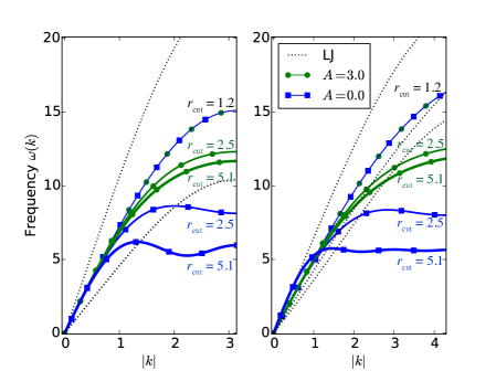
Figure 1: Spectra of the Lennard-Jones Hessian in the fcc ground state and of the preconditioner with $A\in\{0,3\}$ and $r_{\rm cut}\in\{1.2,2.5,5.1\}r_{\rm nn}$ (top to bottom, with increasing line thickness). The graphs for $A=0,3$ with $r_{\rm cut}=1.2$ overlap. Left panel: $(1,1,0)$ direction, Right panel: $(2.7,4.2,3.0)$ direction.

II.5 Default Parameters

The parameters $A$ and $r_{\rm cut}$ are user inputs, however $P$ is fairly insensitive to their choice, provided their interdependency illustrated in Figure 1 is taken into account. Hence, we suggest generic default parameters below. The parameters $\mu$ and $r_{\rm nn}$ are computed in a preprocessing step from the initial configuration of the optimisation.

1. The nearest-neighbour distance $r_{\rm nn}$ is obtained as the maximum of nearest neighbour bond-lengths: if $r_{\rm nn}^{(i)}=\min_{j\neq i}r_{ij}$ then $r_{\rm nn}=\max_{i}r_{\rm nn}^{(i)}$.

2. The exponent $A$ should be large enough to ensure that nearest neighbours dominate, but not so large that small changes in the configuration lead to large changes in $P$. All our tests are performed with $A=0$ and $A=3$; with $A=3$ giving slightly better performance.

3. The cut-off $r_{\rm cut}$ should be larger than $r_{\rm nn}$, however, then exponential decay of the preconditioner entries ensures that additional entries have a small influence. For $A=0$ we choose $r_{\rm cut}=1.1r_{\rm nn}$ and when $A=3$ we use $r_{\rm cut}=2r_{\rm nn}$. The latter choice is intuitively preferable since it accommodates the possibility of significant bond stretching.

4. Finally, the energy-scale $\mu$ is chosen to ensure that the LBFGS algorithm can choose the unit step-length as the default. We achieve this by equating

$$v^{T}\big{(}\nabla E(x_{0}+v)-\nabla E(x_{0})\big{)}=\mu v^{T}P_{\mu=1}v,$$ (14)

where $P_{\mu=1}$ is the metric with $\mu=1$ and $v$ is a test displacement of the form

$$v(x,y,z)=M\big{(}\sin(x/L_{x}),\sin(y/L_{y}),\sin(z/L_{z})\big{)},$$ (15)

where $L_{i}$ are the lengths of the periodic lattice vectors and $M$ is a user-defined matrix with default value $M=10^{-2}r_{\rm nn}I$.

II.6 Implementation details

Preconditioner application. It is important that the cost of applying the preconditioner does not dominate the cost of the calculation over the evaluation of energy and gradient. For inexpensive models (Lennard-Jones, EAM, Stillinger–Weber, etc) the choice of method to solve $z=P_{k}^{-1}q$ in (11) is crucial. Our implementation uses a smoothed aggregation algebraic multigrid method Bell, Olson, and Schroder (2011). As a further optimisation we only rebuild the preconditoner when the maximum atomic displacement since the last update exceeds $r_{nn}/2$.

Line search. Irrespective of the choice of the search direction used (e.g., SD (8), CG Nocedal and Wright (2006) or LBFGS (12)) a line search algorithm must be implemented to choose the length of the step, $\alpha_{k}$. The standard choice is a bracketing algorithm which enforces sufficient decrease and approximate orthogonality between subsequent directions (Wolfe conditions). We observed in our tests that a backtracking algorithm imposing only sufficient decrease (Armijo condition), although less robust in theory, was more efficient in practise. We give the details of our implementation, and additional discussion, in Appendix A.

Robust energy differences. The computation of the energy differences and inner products in the Wolfe conditions (18, 19) must be performed with a high degree of accuracy, since the optimization algorithm relies on robustly detecting the change in energy. A common difficulty in implementing a line search strategy based on (18, 19) is the numerical round-off error that arises for large numbers of atoms (typically $10^{5}$ or higher). Numerically robust inner products are equally important in the inversion of the preconditioner and in the LBFGS algorithm. Numerically robust evaluation of energy differences and inner products may, for example, be implemented using compensated summation algorithms.Higham (2002) A simpler strategy which proved sufficient in our case is to use 128 bit floating point numbers for these steps.

Stabilisation. If the system contains clamped atoms then the preconditioner defined in (13) is strictly positive definite but in order to improve its conditioning and ensure positive definiteness for cases where there are no clamped atoms, we stabilize the preconditioner by adding a diagonal term,

$$\begin{split}P_{ij}&=\left\{\begin{array}[]{cc}-\mu c_{ij}&|r_{ij}|<r_{\mathrm{cut}}\\ 0&|r_{ij}|\geq r_{\mathrm{cut}}\end{array}\right.,\\ P_{ii}&=-\sum_{j\neq i}P_{ij}+\mu C_{\mathrm{stab}}.\end{split}$$ (16)

In all our results we choose $C_{\mathrm{stab}}=0.1$. Even when there are clamped atoms, we find that setting $C_{\mathrm{stab}}=0.1$ improves overall performance.

Variable cell optimisation. We confirmed that our preconditoner also gives good performance when degrees of freedom associated with the periodic unit cell are included as well as the atomic positions. Following the approach of Tadmor et al. Tadmor et al. (1999), we consider a combined objective function $\Phi(x,D)=f(Dx)$ with $3N+9$ degrees of freedom: $3N$ for the atomic positions $x$ and 9 components of the deformation tensor $D$, which is with respect to the original undeformed unit cell. The combined gradient is then given by

$$\nabla_{x,D}\,\Phi(x,D)=\left(D\nabla_{x}f(x),\;\frac{V}{\mu_{c}}\sigma\left(D^{-1}\right)^{T}\right)$$ (17)

where $V$ is the cell volume and $\sigma$ the stress tensor, and we have introduced an additional preconditioner parameter $\mu_{c}$ to set the energy scale for the cell degrees of freedom. $\mu_{c}$ can be pre-computed at the same time as $\mu$ for no additional cost by including a trial perturbation of the cell in (15), with default $v(x_{c})=M/r_{nn}=10^{-2}I$.

III Results

We have selected a broad range of materials examples to test our preconditioner. The first is a 160 Si atom $1\times 1\times 20$ supercell of the cubic diamond structure cell in a slab geometry, with periodic boundary conditions along $x$ and $y$ and free boundaries in $z$, simulated with the Stillinger-Weber interatomic potential.Stillinger and Weber (1985) The two halves of the cell (along $z$) are uniformly displaced toward each other by 0.5 Å, creating a large but very localized strain in the center of the slab. The problem is ill-conditioned because the initial strain is localized, but reaching the relaxed geometry requires all the slab atoms to move out towards the free surfaces. As shown in Fig. 2, both the $A=0$ and $A=3$ preconditioners dramatically reduce the computational cost of the minimization, by a factor of about 6 compared to the non-preconditioned minimizer. Results using the Pfrommer et al. (1997) block-diagonal approximation to the initial inverse Hessian are also shown for comparison. Note that even for this relatively fast interatomic potential the computational cost of applying the preconditioner is nearly negligible, so the reduction in computational time is nearly equal to the reduction in number of energy evaluations.

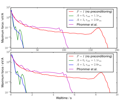
Figure 2: Convergence of the geometry optimisation of a 160-atom silicon slab using the Stillinger-Weber potential in fixed unit cell. The parameters of the preconditioner (or not using a preconditioner) are given in the legend. The lower panel shows the time required to solve the problem in each case, indicating that the overhead of constructing and applying the preconditioner is minimal in comparison to the cost of computing forces with the interatomic potential.

Next we consider a 33,696-atom Si model of the $(111)[11\bar{2}]$ cleavage system (Fig. 3) in a quasi-two-dimensional thin strip geometry with dimensions $717\times 242\times 3.84$ Å³. The applied strain was chosen so that the crack is lattice trapped Thomson, Hsieh, and Rana (1971), leading to a stable ground state with the Stillinger-Weber Stillinger and Weber (1985) interatomic potential. Strong coupling between length scales makes this a difficult system to optimize and hence a good test of our preconditioner. A complex trade off between local chemical cost and long-range elastic relaxation makes it favourable for a 5–7 crack tip reconstruction to form via a bond rotation.Kermode et al. (2008) Here, we find that both the $A=0$ and $A=3$ preconditioners lead to a significant speed up over both unpreconditoned LBFGS and the approach of Pfrommer et al. (1997). Fig. 3 also includes a comparison between the Armijo and Wolfe line searches. As noted above, enforcing only the Armijo condition leads to a further increase in performance.

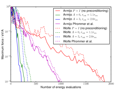
Figure 3: Convergence of the geometry optimisation of a silicon crack using the Stillinger-Weber potential in a fixed unit cell with 33,696 atoms. Solid and dashed lines correspond to using line searches enforcing Armijo and Wolfe conditions, respectively. The parameters of the preconditioner (or not using a preconditioner) are given in the legend.

To investigate whether the theoretical independence of the cost of preconditioned minimisations from system size (Eq. 5) is achieved in real systems, we carried out tests in a series of $N\times 1\times 1$ Si supercells, again using the Stillinger-Weber potential. The atomic positions were perturbed by random displacements of magnitude 0.1 Å and also subjected to a compressive strain of 0.5% to introduce a long-wavelength deformation. The results shown in Fig. 4 indicate that our preconditioner achieves convergence after an approximately constant number of force evaluations as the system is made larger, in contrast to not using a preconditioner or to the approach of Pfrommer et al. (1997) which does not use connectivity information. Our new method is therefore expected to be particularily useful for very large systems.

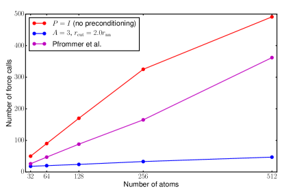
Figure 4: Scaling with system size for geometry optimisations in $N\times 1\times 1$ Si supercells containing from 32 to 512 atoms with the Stillinger-Weber potential, using unpreconditioned LBFGS (red), the inverse Hessian approximation of Pfrommer et al. (magenta), and our new preconditioner (blue).

Since large systems inherently have a wide range of displacement wavelengths and corresponding stiffnesses, it is not obvious a priori how much preconditioning will help for a smaller system, for example one that can feasibly be simulated using density functional theory. We therefore simulated a perovskite structure oxide, LaAlO₃, in a 220-atom slab geometry with periodic boundary conditions in-plane and free surfaces separated by a vacuum region in the normal direction. Energy and force evaluations used DFT with the PBE exchange correlation functional, projector-augmented waves (PAW) with a 282.8 eV cutoff plane-wave basis, and a $2\times 2\times 1$ Monkhorst-Pack k-point sampling, evaluated using the QUIP interface to the VASP software.Csányi et al. (2007); Kresse and Hafner (1994); Kresse and Furthmüller (1996) In this system, as shown in Fig. 5, we find that the preconditioning still significantly reduces the computational cost, but the improvement is not as dramatic as for the larger systems discussed above. With our convergence criterion the reduction is about a factor of two, although the non-preconditioned minimization stagnates just before reaching convergence, and with a slightly looser criterion the reduction would only be a factor of 1.6. Note that the computational cost of the DFT energy and force evaluations is so large that the application of the preconditioner is completely negligible in comparison. In this case the approach of Pfrommer et al. (1997) does not make a significant improvemenet over not using a preconditioner.

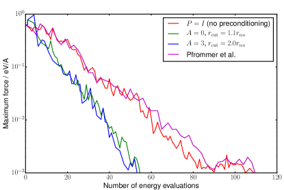
Figure 5: Convergence of the geometry optimisation of a 220-atom LaAlO₃ slab using DFT in a fixed unit cell. The parameters of the preconditioner (or not using a preconditioner) are given in the legend.

For a test of the relaxation of both atomic positions and unit cell size and shape we used a $1\times 1\times 2$ supercell of a $\gamma$-Al₂O₃ structure, with methods similar to those described above for LaAlO₃, except for a 530 eV plane wave cutoff and a $\Gamma$-centered k-point mesh. For this system, plotted in Fig. 6, the reduction in computations for both preconditioners is about a factor of 5, a very significant improvement. While the non-preconditioned minimizer fails to make progress at several points during the relaxation, both our new preconditioners allow the LBFGS minimizer to rapidly and steadily reduce the gradient until convergence. Here, the approach of Pfrommer et al. (1997) actually results in slightly worse performance than unpreconditioned LBFGS. This could perhaps be improved by careful tuning of the bulk modulus and optical phonon frequency parameters used to construct the approximation to the inverse Hessian; however, we note that our new preconditioner does not require any user input as all parameters are computed automatically. The addition of the cell degrees of freedom, which are preconditioned in magnitude but not coupled to the positional degrees of freedom, do not reduce the effectiveness of our preconditioners.

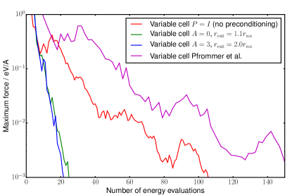
Figure 6: Convergence of the geometry optimisation of a 106-atom $\gamma$-Al₂O₃ system in a variable cell. The parameters of the preconditioner (or not using a preconditioner) are given in the legend.

Finally we tested the new preconditioner for a molecular system, ice VIII. The system contained 432 atoms with an initial cell dimension of $13.65\times 13.65\times 13.16$ ų. A DFT potential with BLYP exchange-correlation functional was used with DZVP basis set and GTH pseudopotentials. Calculations were performed by the CP2K program package using the QUIP interface.Csányi et al. (2007); VandeVondele et al. (2005); Hutter et al. (2014) Fig. 7 shows the number of energy evaluations of the different optimisations for fixed and variable cells using a maximum force threshold of $10^{-3}$ eV Å^-1. Similarly to previous systems, the Armijo condition performed better than Wolfe so we present here only the results with the former line search. In the $A=0$ case we slightly increased the default cutoff parameter ($r_{\rm{cut}}=2.25$ Å) to include hydrogen bonded neighbours too. For both the fixed and variable cells the computational costs compared to the unpreconditioned optimisation were reduced by 3 and 4 times using $A=0$ and $A=3$, respectively.

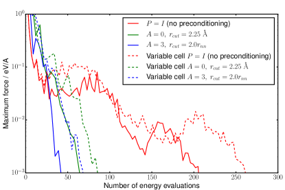
Figure 7: Convergence of the geometry optimisation of a 432-atom ice VIII system with fixed (solid lines) and variable (dashed lines) unit cells. The parameters of the preconditioner (or not using a preconditioner) are given in the legend.

IV Saddle search

To demonstrate the transferability of our preconditioner not only across problem classes but also across algorithms, we apply it to the dimer saddle search algorithm.Henkelman and Jónsson (1999); Gould, Ortner, and Packwood A modified variant of the algorithm proposed in Ref. Gould, Ortner, and Packwood, reads

$$x_{k+1} =x_{k}-\alpha\big{(}P_{k}^{-1}-2v_{k}v_{k}^{T}\big{)}{\textstyle\frac{\nabla f(x_{k}+hv_{k})+\nabla f(x_{k}-hv_{k})}{2}},$$

$$v_{k+1}^{\prime} =v_{k}-\beta\big{(}I-P_{k}v_{k}v_{k}^{T}\big{)}{\textstyle\frac{\nabla f(x_{k}+hv_{k})-\nabla f(x_{k}-hv_{k})}{2h}},$$

$$v_{k+1} =v_{k+1}^{\prime}/\|v_{k+1}^{\prime}\|_{P_{k+1}}.$$

The translation step is obtained as coordinate transformation of the standard dimer step with the variables $\tilde{x}_{k}=P_{k}^{1/2}x_{k},\tilde{v}_{k}=P_{k}^{1/2}v_{k}$ (cf. §II.2). The orientation step is an $\ell^{2}$-steepest descent step (without preconditioning) for the Rayleigh-quotient $v^{T}\nabla^{2}f(x_{k})v/v^{T}P_{k}v$, with a finite-difference approximation of $\nabla^{2}f(x_{k})v$. Interestingly, naive preconditioning of the orientation steps led to poorer performance in our tests.

We test this preconditioned dimer algorithm by computing the saddle configuration of a vacancy in a Lennard-Jones fcc crystal, with a cubic computational cell. Given two states $x^{(0)},x^{(1)}$ which have two neighbouring lattice sites removed, we choose the starting configuration $x_{0}=\frac{1}{3}x^{(0)}+\frac{2}{3}x^{(1)}$ and $v_{0}\propto x^{(1)}-x^{(0)}$. The step-sizes are chosen by hand-optimising for a small setup with $3^{3}$ unit cells: $\alpha=0.01,\beta=0.005$ for the unpreconditioned variant ($P_{k}=I$) and $\alpha=0.5,\beta=0.01$ for our preconditioner with parameters $A=3.0,r_{\rm rcut}=2r_{\rm nn}$. For both variants we chose $h=10^{-2}$. The results are displayed in Figure 8, demonstrating analogous improvements to the energy minimisation examples.

Figure 8: Performance of the preconditioned dimer method for a vacancy in a Lennard-Jones fcc crystal (solid lines), and without a preconditioner (dashed lines), for two system sizes.

V Conclusions

In summary, we have presented a simple preconditioner for geometry optimisation and saddle search that is universally applicable in a wide range of atomistic and molecular condensed phase systems, offering at least a factor of two in performance gain in our examples of small systems, and up to factor of ten in systems of tens of thousands of atoms. The extra cost of using the preconditioner is small enough that it is worth using even with inexpensive interatomic potentials, while the performance gain is expected to scale as the square root of the system size. A Python implementation within the Atomic Simulation EnvironmentBahn and Jacobsen (2002) is available at https://gitlab.com/jameskermode/ase, offering interfaces to a wide range of atomistic codes such as VASPKresse and Hafner (1994), CASTEPClark et al. (2005), CP2KVandeVondele et al. (2005), LAMMPSPlimpton (1995), and many others.

Appendix A Linesearch

We present the details of our line search algorithm. The standard requirement for the LBFGS and CG methods is that the step-size, $\alpha$, satisfies the Wolfe conditions

$$f(x_{k}+\alpha p_{k}) \leq f(x_{k})+c_{1}\alpha\nabla f_{k}^{T}p_{k},$$ (18)

$$|\nabla f(x_{k}+\alpha p_{k})^{T}p_{k}| \leq c_{2}|\nabla f_{k}^{T}p_{k}|,$$ (19)

where $0<c_{2}<c_{1}<1$. Line search methods that guarantee (18) and (19) employ a bracketing strategy, which often requires several additional energy and force evaluations at each iteration.

For the steepest descent method it is theoretically sufficient to impose only the Armijo condition (18). We have observed that this was also sufficient in all our tests to ensure convergence of the LBFGS method and leads to a consistent performance improvement. Our implementation minimises the quadratic interpolating $f_{k},\nabla f_{k}^{T}p_{k}$ and $f(x_{k}+\alpha p_{k})$, iterating until (18) is satisfied. For $c_{1}<1/2$ this yields a backtracking guarantee and hence ensures that the line search terminates after finitely many steps. Our default parameter is $c_{1}=0.1$. The initial estimate on the step-length is $\tilde{\alpha}=1.0$.

$$\begin{split}&{\bf input}~{}x,\tilde{\alpha}>0,c_{1}\in(0,1/2),p\text{ s.t. }\nabla f(x)\cdot p<0.\\ &{\bf output}~{}\tilde{\alpha}.\\ &\mathrm{while}\>f(x+\tilde{\alpha}p)>f(x)+c_{1}\tilde{\alpha}\nabla f(x)\cdot p\\ &\qquad\tilde{\alpha}^{\prime}\leftarrow\frac{-\frac{1}{2}\tilde{\alpha}\nabla f(x)\cdot p}{\frac{f(x+\tilde{\alpha}p)-f(x)}{\tilde{\alpha}}-\nabla f(x)\cdot p}\\ &\qquad\tilde{\alpha}\leftarrow\max(\tilde{\alpha}^{\prime},\tilde{\alpha}/10)\end{split}$$ (20)

Unlike for a bracketing line-search, the only additional evaluations required during line search are energy evaluations at the end-point of the search interval, which reduces computational cost in the pre-asymptotic regime of the optimisation.

In the asymptotic regime, the step-length $\alpha_{k}=1$ is always accepted, and will satisfy both Wolfe conditions (18) and (19) provided that $c_{1}<1/2$. Since, through the use of our proposed preconditioner, we substantially reduce the number of iterations, it is unlikely that the potential instabilities associated with Armijo line search for the LBFGS direction will be observed. Moreover, in our implementation, if the Armijo linesearch fails we simply reset the LBFGS Hessian history and repeat the linesearch, which removes any concern about robustness.

Appendix B Phonon Stability

Consider a $d$-dimensional Bravais lattice $\Lambda=A\mathbb{Z}^{d}$, where $\mathbb{Z}$ is the set of integers and the columns of $A$ are the lattice directions, which is the ground state for some material system under a potential energy $f$. Let $H=\nabla^{2}f$ denote the Hessian of the potential energy in the ground state. For displacements $u_{r}$ of each atom $r\in\Lambda$ we can write

$$[Hu]_{r}=\sum_{s\in\Lambda}H_{rs}u_{s},$$ (21)

where $H_{rs}\in\mathbb{R}^{d\times d}$ are the blocks of $H$. We now prove the claim that phonon stability is equivalent to the bound $u^{T}Hu\geq u^{T}Pu$, where $P$ is the preconditioner defined in (13), for all displacements of the lattice.

The discrete translation invariance of the lattice, $\Lambda+r=\Lambda$ for all $r\in\Lambda$, implies that $H_{rs}=H_{0,s-r}=:h_{s-r}$ where $h\in\mathbb{R}^{d\times d}$. For any virtual displacement $u=(u_{r})$ with compact support we have

$$u^{T}Hu=\int_{\rm BZ}\hat{u}^{*}\hat{h}\hat{u}\,dk,$$ (22)

where $\hat{u}$ and $\hat{h}$ denote the Fourier transforms of $u$ and $h$, respectively and the integration is over the first Brillouin zone. Phonon stability means that the natural frequencies are positive and linear near the origin. In terms of $\hat{h}$, this translates to $\hat{h}(k)\geq c_{H}|k|^{2}I$ for some constant $c_{H}>0$. The upper bound $\hat{h}(k)\leq C_{H}|k|^{2}I$ follows from the boundedness of the phonon band width. (A sufficient condition is that $\sum_{r\in\Lambda}|h_{r}||r|^{2}<\infty$.)

Let $P_{rs}=p_{s-r}\in\mathbb{R}^{d\times d}$ denote the corresponding blocks of the preconditioner operator. The upper bound $\hat{p}\leq C_{P}|k|^{2}I$ follows simply from the fact that the preconditioner has a finite interaction range. This upper bound and phonon stability of $H$ imply

$$u^{T}Hu \geq c_{H}\int_{\rm BZ}|k|^{2}|\hat{u}|^{2}dk$$

$$\geq\frac{c_{H}}{C_{P}}\int_{\rm BZ}\hat{u}^{*}\hat{p}\hat{u}$$

$$=\frac{c_{H}}{C_{P}}u^{T}Pu.$$

Conversely, if $u^{T}Hu\geq cu^{T}Pu$, then phonon stability of $P$ implies phonon stability of $H$. But the former is an immediate consequence of the fact that the coefficients in the definition of $P$ are positive.Born and Huang (1998)

References

- Wales (2003) D. Wales, Energy landscapes: Applications to clusters, biomolecules and glasses (Cambridge University Press, 2003).
- Pickard and Needs (2011) C. J. Pickard and R. J. Needs, J. Phys. Condens. Matter 23, 053201 (2011).
- Voter (1997) A. Voter, Phys. Rev. Lett. 78, 3908 (1997).
- Payne et al. (1992) M. C. Payne, M. P. Teter, D. C. Allan, T. A. Arias, and J. D. Joannopoulos, Rev. Mod. Phys. 64, 1045 (1992).
- Elman, Silvester, and Wathen (2014) H. C. Elman, D. J. Silvester, and A. J. Wathen, Finite elements and fast iterative solvers: with applications in incompressible fluid dynamics (Oxford University Press, 2014).
- Nocedal and Wright (2006) J. Nocedal and S. J. Wright, Numerical Optimisation, Springer Series in Operations Research and Financial Engineering (Springer New York, 2006).
- Pfrommer et al. (1997) B. G. Pfrommer, M. Côté, S. G. Louie, and M. L. Cohen, J. Comput. Phys. 131, 233 (1997).
- Fernandex-Serra, Artacho, and Soler (2013) M. V. Fernandex-Serra, E. Artacho, and J. M. Soler, Phys. Rev. B 67, 100101 (2013).
- Bertsekas (1999) D. P. Bertsekas, Nonlinear Programming 2nd Edition (Athena Scientific, 1999).
- Bell, Olson, and Schroder (2011) W. N. Bell, L. N. Olson, and J. B. Schroder, “PyAMG: Algebraic multigrid solvers in Python v2.0,” (2011), release 2.0.
- Higham (2002) N. Higham, Accuracy and Stability of Numerical Algorithms (SIAM, 2002).
- Tadmor et al. (1999) E. B. Tadmor, G. S. Smith, N. Bernstein, and E. Kaxiras, Phys. Rev. B Condens. Matter 59, 235 (1999).
- Stillinger and Weber (1985) F. H. Stillinger and T. A. Weber, Phys. Rev. B Condens. Matter 31, 5262 (1985).
- Thomson, Hsieh, and Rana (1971) R. Thomson, C. Hsieh, and V. Rana, J. Appl. Phys. 42, 3154 (1971).
- Kermode et al. (2008) J. R. Kermode, T. Albaret, D. Sherman, N. Bernstein, P. Gumbsch, M. C. Payne, G. Csányi, and A. De Vita, Nature 455, 1224 (2008).
- Csányi et al. (2007) G. Csányi, S. Winfield, J. Kermode, A. De Vita, A. Comisso, N. Bernstein, and M. Payne, IoP Comput. Phys. Newsl. Spring 2007 (2007).
- Kresse and Hafner (1994) G. Kresse and J. Hafner, Phys. Rev. B Condens. Matter 49, 14251 (1994).
- Kresse and Furthmüller (1996) G. Kresse and J. Furthmüller, Phys. Rev. B Condens. Matter 54, 11169 (1996).
- VandeVondele et al. (2005) J. VandeVondele, M. Krack, F. Mohamed, M. Parrinello, T. Chassaing, and J. Hutter, Comput. Phys. Commun. 167, 103 (2005).
- Hutter et al. (2014) J. Hutter, M. Iannuzzi, F. Schiffmann, and J. VandeVondele, Wiley Interdiscip. Rev. Comput. Mol. Sci. 4, 15 (2014).
- Henkelman and Jónsson (1999) G. Henkelman and H. Jónsson, Journal of Chemical Physics 111, 7010 (1999).
- (22) N. Gould, C. Ortner, and D. Packwood, “An efficient dimer method with preconditioning and linesearch,” Arxiv:1407.2817, to appear in Math. Comp.
- Bahn and Jacobsen (2002) S. R. Bahn and K. W. Jacobsen, Comput. Sci. Eng. 4, 56 (2002).
- Clark et al. (2005) S. J. Clark, M. D. Segall, C. J. Pickard, P. J. Hasnip, M. I. J. Probert, K. Refson, and M. C. Payne, Z. Kristallogr. 220, 567 (2005).
- Plimpton (1995) S. Plimpton, J. Comp. Phys. 117, 1 (1995).
- Born and Huang (1998) M. Born and K. Huang, Dynamical Theory of Crystal Lattices (Clarendon Press, 1998).